Exploring the Revenue-Generating Potential of AI Factories

Exploring the Revenue-Generating Potential of AI Factories

AI is creating value for everyone — from researchers in drug discovery to quantitative analysts navigating financial market changes.

The faster an AI system can produce tokens, a unit of data used to string together outputs, the greater its impact. That’s why AI factories are key, providing the most efficient path from “time to first token” to “time to first value.”

AI factories are redefining the economics of modern infrastructure. They produce intelligence by transforming data into valuable outputs — whether tokens, predictions, images, proteins or other forms — at massive scale.

They help enhance three key aspects of the AI journey — data ingestion, model training and high-volume inference. AI factories are being built to generate tokens faster and more accurately, using three critical technology stacks: AI models, accelerated computing infrastructure and enterprise-grade software.

Read on to learn how AI factories are helping enterprises and organizations around the world convert the most valuable digital commodity — data — into revenue potential.

From Inference Economics to Value Creation

Before building an AI factory, it’s important to understand the economics of inference — how to balance costs, energy efficiency and an increasing demand for AI.

Throughput refers to the volume of tokens that a model can produce. Latency is the amount of tokens that the model can output in a specific amount of time, which is often measured in time to first token — how long it takes before the first output appears — and time per output token, or how fast each additional token comes out. Goodput is a newer metric, measuring how much useful output a system can deliver while hitting key latency targets.

User experience is key for any software application, and the same goes for AI factories. High throughput means smarter AI, and lower latency ensures timely responses. When both of these measures are balanced properly, AI factories can provide engaging user experiences by quickly delivering helpful outputs.

For example, an AI-powered customer service agent that responds in half a second is far more engaging and valuable than one that responds in five seconds, even if both ultimately generate the same number of tokens in the answer.

Companies can take the opportunity to place competitive prices on their inference output, resulting in more revenue potential per token.

Measuring and visualizing this balance can be difficult — which is where the concept of a Pareto frontier comes in.

AI Factory Output: The Value of Efficient Tokens

The Pareto frontier, represented in the figure below, helps visualize the most optimal ways to balance trade-offs between competing goals — like faster responses vs. serving more users simultaneously — when deploying AI at scale.

The vertical axis represents throughput efficiency, measured in tokens per second (TPS), for a given amount of energy used. The higher this number, the more requests an AI factory can handle concurrently.

The horizontal axis represents the TPS for a single user, representing how long it takes for a model to give a user the first answer to a prompt. The higher the value, the better the expected user experience. Lower latency and faster response times are generally desirable for interactive applications like chatbots and real-time analysis tools.

The Pareto frontier’s maximum value — shown as the top value of the curve — represents the best output for given sets of operating configurations. The goal is to find the optimal balance between throughput and user experience for different AI workloads and applications.

The best AI factories use accelerated computing to increase tokens per watt — optimizing AI performance while dramatically increasing energy efficiency across AI factories and applications.

The animation above compares user experience when running on NVIDIA H100 GPUs configured to run at 32 tokens per second per user, versus NVIDIA B300 GPUs running at 344 tokens per second per user. At the configured user experience, Blackwell Ultra delivers over a 10x better experience and almost 5x higher throughput, enabling up to 50x higher revenue potential.

How an AI Factory Works in Practice

An AI factory is a system of components that come together to turn data into intelligence. It doesn’t necessarily take the form of a high-end, on-premises data center, but could be an AI-dedicated cloud or hybrid model running on accelerated compute infrastructure. Or it could be a telecom infrastructure that can both optimize the network and perform inference at the edge.

Any dedicated accelerated computing infrastructure paired with software turning data into intelligence through AI is, in practice, an AI factory.

The components include accelerated computing, networking, software, storage, systems, and tools and services.

When a person prompts an AI system, the full stack of the AI factory goes to work. The factory tokenizes the prompt, turning data into small units of meaning — like fragments of images, sounds and words.

Each token is put through a GPU-powered AI model, which performs compute-intensive reasoning on the AI model to generate the best response. Each GPU performs parallel processing — enabled by high-speed networking and interconnects — to crunch data simultaneously.

An AI factory will run this process for different prompts from users across the globe. This is real-time inference, producing intelligence at industrial scale.

Because AI factories unify the full AI lifecycle, this system is continuously improving: inference is logged, edge cases are flagged for retraining and optimization loops tighten over time — all without manual intervention, an example of goodput in action.

Leading global security technology company Lockheed Martin has built its own AI factory to support diverse uses across its business. Through its Lockheed Martin AI Center, the company centralized its generative AI workloads on the NVIDIA DGX SuperPOD to train and customize AI models, use the full power of specialized infrastructure and reduce the overhead costs of cloud environments.

“With our on-premises AI factory, we handle tokenization, training and deployment in house,” said Greg Forrest, director of AI foundations at Lockheed Martin. “Our DGX SuperPOD helps us process over 1 billion tokens per week, enabling fine-tuning, retrieval-augmented generation or inference on our large language models. This solution avoids the escalating costs and significant limitations of fees based on token usage.”

NVIDIA Full-Stack Technologies for AI Factory

An AI factory transforms AI from a series of isolated experiments into a scalable, repeatable and reliable engine for innovation and business value.

NVIDIA provides all the components needed to build AI factories, including accelerated computing, high-performance GPUs, high-bandwidth networking and optimized software.

NVIDIA Blackwell GPUs, for example, can be connected via networking, liquid-cooled for energy efficiency and orchestrated with AI software.

The NVIDIA Dynamo open-source inference platform offers an operating system for AI factories. It’s built to accelerate and scale AI with maximum efficiency and minimum cost. By intelligently routing, scheduling and optimizing inference requests, Dynamo ensures that every GPU cycle ensures full utilization, driving token production with peak performance.

NVIDIA Blackwell GB200 NVL72 systems and NVIDIA InfiniBand networking are tailored to maximize token throughput per watt, making the AI factory highly efficient from both total throughput and low latency perspectives.

By validating optimized, full-stack solutions, organizations can build and maintain cutting-edge AI systems efficiently. A full-stack AI factory supports enterprises in achieving operational excellence, enabling them to harness AI’s potential faster and with greater confidence.

Learn more about how AI factories are redefining data centers and enabling the next era of AI.

Read More

Time to Slay: ‘DOOM: The Dark Ages’ Looms on GeForce NOW

Time to Slay: ‘DOOM: The Dark Ages’ Looms on GeForce NOW

Steel clashes and war drums thunder as a new age of battle dawns — one that will test even the mightiest Slayer.

This GFN Thursday, DOOM: The Dark Ages — the bold medieval-inspired prequel to DOOM and DOOM Eternal — is available for GeForce NOW premium members, aka Ultimate and Performance members, to stream from the cloud at launch. Premium members can also slay in style with a free in-game reward.

The stage is set and the crowd is buzzing — Capcom: Fighting Collection 2 is joining GeForce NOW at launch.

Plus, get ready to take to the skies with Microsoft Flight Simulator 2024 coming to the cloud this week.

And catch the latest GeForce NOW updates rolling out to members starting this week. The updates include quality-of-life improvements, following performance enhancements like 120 frames-per-second streaming for SHIELD TV to keep the cloud gaming experience at its best.

It’s all part of another thrilling GFN Thursday, with five new games joining the cloud.

Stand and Fight

DOOM The Dark Ages on GeForce NOW
Keep your friends close and your enemies closer.

DOOM: The Dark Ages is a dark fantasy and sci-fi single-player experience that delivers the searing combat and over-the-top visuals of the DOOM franchise, powered by the latest idTech engine.

As the super weapon of gods and kings, shred enemies with devastating favorites like the Super Shotgun while wielding a variety of new bone-chewing weapons, including the versatile Shield Saw. Players will stand and fight on the demon-infested battlefields in the vicious, grounded combat the original DOOM is famous for. Take flight atop the new fierce Mecha Dragon, stand tall in a massive Atlan mech and beat demons to a pulp with the newly enhanced glory kill system. Only the Slayer has the power to wield these devastating tools of mayhem.

Experience every gory detail, thunderous shield bash and demon-splitting kill in the cloud. No downloads, no waiting — just pure, uninterrupted DOOM action, wherever members want to play.

DOOM reward on GeForce NOW
SHIELD your eyes.

GeForce NOW Ultimate or Performance members can now claim the DOOM Slayer Verdant skin reward, a fierce, ruthless-looking armor set that’s built for relentless slaughter. Those who’ve opted in to GeForce NOW’s Rewards program can check their email for instructions on how to redeem it. It’s available through Sunday, June 15, first come, first served.

Step Into the Ring

Capcom Fighting Collection 2
The fight continues.

Capcom’s new fighting collection hits the stage — and the cloud.

Choose from fan favorites like Capcom vs. SNK 2: Mark of the Millennium 2001 and Project Justice, as well as 3D action titles like Power Stone and Power Stone 2 in this collection of eight classic fighting games. Each can be played online or in co-op mode. Get back in the ring and duke it out in battles that everyone rumored but no one believed.

Chase victory by streaming on GeForce NOW. Ultimate and Performance members enjoy higher resolutions and lower latency compared with free users for a true cloud-gaming edge.

Game On

Streaming from a powerful GeForce RTX gaming rig in the cloud enables GeForce NOW to deliver continuous improvements and new features that enhance members’ streaming experiences. This week, update 2.0.74 is rolling out, bringing several enhancements to the cloud.

Members will see an upgraded library syncing feature for those using PC game subscription services like PC Game Pass and Ubisoft+, making it even easier to jump into games. Supported titles for these game services will now be automatically added to members’ “My Library” after resyncing their Ubisoft, Battle.net and Xbox connected accounts in the GeForce NOW app.

This update follows the recent performance boost for SHIELD TV users in SHIELD Experience 9.2.1, now supporting up to 120 fps 1080p streaming for GeForce NOW Ultimate members. Those who prefer higher resolution over frame rates can continue streaming at up to 4K 60 fps.

With such ongoing updates, GeForce NOW is making cloud gaming more seamless and accessible across devices.

Fly Your Way

Microsoft Flight Simulator 2024 on GeForce NOW
Fly anywhere with the cloud.

GeForce NOW brings a groundbreaking aviation experience to the cloud with Microsoft Flight Simulator 2024. Members can experience the game that redefines aviation simulation with unparalleled realism and global exploration.

Pursue dynamic aviation careers through missions like Medevac, Search and Rescue, and Aerial Firefighting. Plus, compete in thrilling events such as the Red Bull Air Races. The game introduces advanced physics, enhanced aircraft systems and a groundbreaking flight planner for immersive gameplay. Explore an exceptionally detailed digital recreation of Earth, featuring handcrafted airports, landmarks, dynamic biomes, and real-time air and maritime traffic.

With stunning visuals, diverse wildlife and realistic weather systems, Microsoft Flight Simulator 2024 offers unmatched experiences for pilots and adventurers. Ultimate and Performance members can play with GeForce RTX 4080-level performance with the highest frame rates and lowest latency. Ultimate members can elevate their adventures at up to 4K resolution and 120 fps for the most immersive rides in the sky.

Fired Up for New Games

Blacksmith Master on GeForce NOW
It’s hammer time.

Manage a medieval forge in Blacksmith Master, launching this week in the cloud. Find and hire the best staff and equip them with the right tools to optimize the business and train their skills over time. Design the shop for the best throughput, fulfill orders from across the kingdom to unlock new capabilities, and seek out new opportunities in the market as customers come looking for a variety of historically inspired items — from weapons and armor to tools and cooking utensils. Perfect the craft to become the Blacksmith Master.

Look for the following games available to stream in the cloud this week:

  • The Precinct (New release on Steam, May 13)
  • Blacksmith Master (New release on Steam, May 15)
  • Capcom Fighting Collection 2 (New release on Steam, May 15)
  • DOOM: The Dark Ages (New release on Steam, Battle.net and Xbox, available on PC Game Pass, May 154)
  • Microsoft Flight Simulator 2024 (Steam and Xbox, available on PC Game Pass)

What are you planning to play this weekend? Let us know on X or in the comments below.

Read More

Into the Omniverse: Computational Fluid Dynamics Simulation Finds Smoothest Flow With AI-Driven Digital Twins

Into the Omniverse: Computational Fluid Dynamics Simulation Finds Smoothest Flow With AI-Driven Digital Twins

Editor’s note: This post is part of Into the Omniverse, a series focused on how developers, 3D practitioners and enterprises can transform their workflows using the latest advances in OpenUSD and NVIDIA Omniverse.

Computer-aided engineering (CAE) is at the forefront of modern product development, enabling engineers to virtually test and refine designs before building physical prototypes. Among the powerful CAE methods, computational fluid dynamics (CFD) simulation plays a critical role in understanding and optimizing fluid flow for use cases, such as aerodynamic testing in aerospace and automotive engineering or thermal management for electronics.

The NVIDIA Omniverse Blueprint for real-time digital twins provides a powerful framework for developers to build complex CFD simulation solutions with the combined power of NVIDIA CUDA-X acceleration libraries, NVIDIA PhysicsNeMo AI framework and NVIDIA Omniverse, and Universal Scene Description (OpenUSD).

Multiphysics simulation generates a high diversity of data with optical, thermal, electromagnetic and mechanical applications, all requiring different inputs and outputs.

OpenUSD provides a unified data model that connects the CAE ecosystem so digital twins can operate in real time with diverse data inputs. This seamless interoperability between tools is crucial for engineering efforts that rely on accurate, consistent CFD simulations.

Industry Leaders Deliver 50x Faster Simulation 

At NVIDIA GTC in March, NVIDIA announced that leading CAE software providers, including Ansys, Altair, Cadence, Siemens and Synopsys, are accelerating their simulation tools, including for CFD, by up to 50x with the NVIDIA Blackwell platform.

Thanks to accelerated software, NVIDIA CUDA-X libraries and performance-optimization blueprints, industries like automotive, aerospace, energy, manufacturing and life sciences can greatly reduce product development time and costs while increasing design accuracy and remaining energy efficient.

Ansys, a leader in simulation software, is harnessing the power of NVIDIA technologies for real-time physics and accelerated simulation with AI-driven digital twins. By integrating NVIDIA GPUs and tapping into Blackwell’s advanced accelerated computing capabilities, Ansys software enables engineers to run complex CFD simulations at unprecedented speed and scale.

Real-Time Digital Twins for CFD

Ansys is also adopting Omniverse and OpenUSD to create more connected, collaborative simulation environments for CFD. Ansys users can build real-time digital twins that integrate data from multiple sources, and now those multidisciplinary CFD simulations can be integrated into the visually rich Omniverse environment.

Learn more about how Ansys is using NVIDIA technologies and OpenUSD to advance its CFD workflows in this livestream replay:

Get Plugged Into the World of OpenUSD

Join NVIDIA GTC Taipei at COMPUTEX, running May 19-23, to see how accelerated computing, Omniverse and OpenUSD advance 3D workflows. Watch NVIDIA founder and CEO Jensen Huang’s COMPUTEX keynote on Monday, May 19, at 11 a.m. Taiwan Time.

Ansys Simulation World is a virtual and in-person global simulation experience. The virtual event takes place July 16-17, and includes a keynote from Huang that will provide a closer look at the transformative power of accelerated computing and AI to enable computational engineering breakthroughs – including CFD – across all industries. Until then, watch Ansys GTC sessions on demand to learn more.

Discover why developers and 3D practitioners are using OpenUSD and learn how to optimize 3D workflows with the new self-paced “Learn OpenUSD” curriculum for 3D developers and practitioners, available for free through the NVIDIA Deep Learning Institute.

For more resources on OpenUSD, explore the Alliance for OpenUSD forum and the AOUSD website.

Stay up to date by subscribing to NVIDIA Omniverse news, joining the community and following NVIDIA Omniverse on Instagram, LinkedIn, Medium and X.

Featured image courtesy of Ansys.

Read More

Visa Makes Payments Personalized and Secure With AI

Visa Makes Payments Personalized and Secure With AI

Think tap to pay — but smarter and safer. Visa is tapping into AI to enhance services for its global network of customers, focused on fraud prevention, personalization and agentic commerce.

Sarah Laszlo, senior director of Visa’s machine learning platform, joined the AI Podcast to discuss how artificial intelligence is powering the next generation of payment experiences.

Visa processes hundreds of billions of transactions each year, so even small technological enhancements can have a large impact.

The company prevents $40 billion in fraud annually. “There’s so much attempted fraud that, even though we’re very good at preventing it, marginal improvements save large dollar amounts,” Laszlo said.

AI also powers Visa’s personalization systems, delivering smarter, more relevant offers and recommendations to cardholders. The company’s unique dataset presents a huge opportunity to improve transaction predictions — but also brings privacy challenges.

“The key to addressing those challenges is building abstract representations of users — embeddings that capture preferences without exposing private data,” Laszlo said.

The company is also working toward agentic commerce — where AI agents help customers with payments. For example, AI agents with access to payment credentials can handle transactions on behalf of consumers, like booking travel arrangements, when instructed.

Laszlo shared best practices for enterprises adopting generative AI. She also recommended using open-source models when possible and developing strong relationships between governance and technical teams. In one success story, Visa used GPT-4 to convert legacy code to Python, saving $5 million, with just one engineer completing 50 conversion jobs in a quarter.

To learn more, watch Laszlo’s GTC session, The Next Era of Payments: How Generative AI is Shaping the Future.

Time Stamps

03:28 – Visa’s priorities for AI use.

07:09 – How Visa optimizes resources using virtual GPUs.

14:42 – AI factories and unified pipelines.

18:52 – Best practices for AI in financial services.

You Might Also Like… 

NVIDIA’s Jacob Liberman on Bringing Agentic AI to Enterprises

Agentic AI enables developers to create intelligent multi-agent systems that reason, act and execute complex tasks with a degree of autonomy. Jacob Liberman, director of product management at NVIDIA, explains how agentic AI bridges the gap between powerful AI models and practical enterprise applications.

Firsthand’s Jon Heller Shares How AI Agents Enhance Consumer Journeys in Retail

Jon Heller, co-CEO and founder of Firsthand, discusses how the company’s Brand Agents are transforming the retail landscape by personalizing customer journeys, converting marketing interactions into valuable research data and enhancing the customer experience with hyper-personalized insights and recommendations.

Telenor Builds Norway’s First AI Factory, Offering Sustainable and Sovereign Data Processing

Telenor opened Norway’s first AI factory in November 2024, enabling organizations to process sensitive data securely on Norwegian soil while prioritizing environmental responsibility. Telenor’s Chief Innovation Officer and Head of the AI Factory Kaaren Hilsen discusses the AI factory’s rapid development, going from concept to reality in under a year.

Read More

Cost-effective AI image generation with PixArt-Σ inference on AWS Trainium and AWS Inferentia

Cost-effective AI image generation with PixArt-Σ inference on AWS Trainium and AWS Inferentia

PixArt-Sigma is a diffusion transformer model that is capable of image generation at 4k resolution. This model shows significant improvements over previous generation PixArt models like Pixart-Alpha and other diffusion models through dataset and architectural improvements. AWS Trainium and AWS Inferentia are purpose-built AI chips to accelerate machine learning (ML) workloads, making them ideal for cost-effective deployment of large generative models. By using these AI chips, you can achieve optimal performance and efficiency when running inference with diffusion transformer models like PixArt-Sigma.

This post is the first in a series where we will run multiple diffusion transformers on Trainium and Inferentia-powered instances. In this post, we show how you can deploy PixArt-Sigma to Trainium and Inferentia-powered instances.

Solution overview

The steps outlined below will be used to deploy the PixArt-Sigma model on AWS Trainium and run inference on it to generate high-quality images.

  • Step 1 – Pre-requisites and setup
  • Step 2 – Download and compile the PixArt-Sigma model for AWS Trainium
  • Step 3 – Deploy the model on AWS Trainium to generate images

Step 1 – Prerequisites and setup

To get started, you will need to set up a development environment on a trn1, trn2, or inf2 host. Complete the following steps:

  1. Launch a trn1.32xlarge or trn2.48xlarge instance with a Neuron DLAMI. For instructions on how to get started, refer to Get Started with Neuron on Ubuntu 22 with Neuron Multi-Framework DLAMI.
  2. Launch a Jupyter Notebook sever. For instructions to set up a Jupyter server, refer to the following user guide.
  3. Clone the aws-neuron-samples GitHub repository:
    git clone https://github.com/aws-neuron/aws-neuron-samples.git

  4. Navigate to the hf_pretrained_pixart_sigma_1k_latency_optimized.ipynb notebook:
    cd aws-neuron-samples/torch-neuronx/inference

The provided example script is designed to run on a Trn2 instance, but you can adapt it for Trn1 or Inf2 instances with minimal modifications. Specifically, within the notebook and in each of the component files under the neuron_pixart_sigma directory, you will find commented-out changes to accommodate Trn1 or Inf2 configurations.

Step 2 – Download and compile the PixArt-Sigma model for AWS Trainium

This section provides a step-by-step guide to compiling PixArt-Sigma for AWS Trainium.

Download the model

You will find a helper function in cache-hf-model.py in above mentioned GitHub repository that shows how to download the PixArt-Sigma model from Hugging Face. If you are using PixArt-Sigma in your own workload, and opt not to use the script included in this post, you can use the huggingface-cli to download the model instead.

The Neuron PixArt-Sigma implementation contains a few scripts and classes. The various files and scrips are broken down as follows:

├── compile_latency_optimized.sh # Full Model Compilation script for Latency Optimized
├── compile_throughput_optimized.sh # Full Model Compilation script for Throughput Optimized
├── hf_pretrained_pixart_sigma_1k_latency_optimized.ipynb # Notebook to run Latency Optimized Pixart-Sigma
├── hf_pretrained_pixart_sigma_1k_throughput_optimized.ipynb # Notebook to run Throughput Optimized Pixart-Sigma
├── neuron_pixart_sigma
│ ├── cache_hf_model.py # Model downloading Script
│ ├── compile_decoder.py # Text Encoder Compilation Script and Wrapper Class
│ ├── compile_text_encoder.py # Text Encoder Compilation Script and Wrapper Class
│ ├── compile_transformer_latency_optimized.py # Latency Optimized Transformer Compilation Script and Wrapper Class
│ ├── compile_transformer_throughput_optimized.py # Throughput Optimized Transformer Compilation Script and Wrapper Class
│ ├── neuron_commons.py # Base Classes and Attention Implementation
│ └── neuron_parallel_utils.py # Sharded Attention Implementation
└── requirements.txt

This notebook will help you to download the model, compile the individual component models, and invoke the generation pipeline to generate an image. Although the notebooks can be run as a standalone sample, the next few sections of this post will walk through the key implementation details within the component files and scripts to support running PixArt-Sigma on Neuron.

Sharding PixArt linear layers

For each component of PixArt (T5, Transformer, and VAE), the example uses Neuron specific wrapper classes. These wrapper classes serve two purposes. The first purpose is it allows us to trace the models for compilation:

class InferenceTextEncoderWrapper(nn.Module):
    def __init__(self, dtype, t: T5EncoderModel, seqlen: int):
        super().__init__()
        self.dtype = dtype
        self.device = t.device
        self.t = t
    def forward(self, text_input_ids, attention_mask=None):
        return [self.t(text_input_ids, attention_mask)['last_hidden_state'].to(self.dtype)]

Please refer to the neuron_commons.py file for all wrapper modules and classes.

The second reason for using wrapper classes is to modify the attention implementation to run on Neuron. Because diffusion models like PixArt are typically compute-bound, you can improve performance by sharding the attention layer across multiple devices. To do this, you replace the linear layers with NeuronX Distributed’s RowParallelLinear and ColumnParallelLinear layers:

def shard_t5_self_attention(tp_degree: int, selfAttention: T5Attention):
    orig_inner_dim = selfAttention.q.out_features
    dim_head = orig_inner_dim // selfAttention.n_heads
    original_nheads = selfAttention.n_heads
    selfAttention.n_heads = selfAttention.n_heads // tp_degree
    selfAttention.inner_dim = dim_head * selfAttention.n_heads
    orig_q = selfAttention.q
    selfAttention.q = ColumnParallelLinear(
        selfAttention.q.in_features,
        selfAttention.q.out_features,
        bias=False, 
        gather_output=False)
    selfAttention.q.weight.data = get_sharded_data(orig_q.weight.data, 0)
    del(orig_q)
    orig_k = selfAttention.k
    selfAttention.k = ColumnParallelLinear(
        selfAttention.k.in_features, 
        selfAttention.k.out_features, 
        bias=(selfAttention.k.bias is not None),
        gather_output=False)
    selfAttention.k.weight.data = get_sharded_data(orig_k.weight.data, 0)
    del(orig_k)
    orig_v = selfAttention.v
    selfAttention.v = ColumnParallelLinear(
        selfAttention.v.in_features, 
        selfAttention.v.out_features, 
        bias=(selfAttention.v.bias is not None),
        gather_output=False)
    selfAttention.v.weight.data = get_sharded_data(orig_v.weight.data, 0)
    del(orig_v)
    orig_out = selfAttention.o
    selfAttention.o = RowParallelLinear(
        selfAttention.o.in_features,
        selfAttention.o.out_features,
        bias=(selfAttention.o.bias is not None),
        input_is_parallel=True)
    selfAttention.o.weight.data = get_sharded_data(orig_out.weight.data, 1)
    del(orig_out)
    return selfAttention

Please refer to the neuron_parallel_utils.py file for more details on parallel attention.

Compile individual sub-models

The PixArt-Sigma model is composed of three components. Each component is compiled so the entire generation pipeline can run on Neuron:

  • Text encoder – A 4-billion-parameter encoder, which translates a human-readable prompt into an embedding. In the text encoder, the attention layers are sharded, along with the feed-forward layers, with tensor parallelism.
  • Denoising transformer model – A 700-million-parameter transformer, which iteratively denoises a latent (a numerical representation of a compressed image). In the transformer, the attention layers are sharded, along with the feed-forward layers, with tensor parallelism.
  • Decoder – A VAE decoder that converts our denoiser-generated latent to an output image. For the decoder, the model is deployed with data parallelism.

Now that the model definition is ready, you need to trace a model to run it on Trainium or Inferentia. You can see how to use the trace() function to compile the decoder component model for PixArt in the following code block:

compiled_decoder = torch_neuronx.trace(
    decoder,
    sample_inputs,
    compiler_workdir=f"{compiler_workdir}/decoder",
    compiler_args=compiler_flags,
    inline_weights_to_neff=False
)

Please refer to the compile_decoder.py file for more on how to instantiate and compile the decoder.

To run models with tensor parallelism, a technique used to split a tensor into chunks across multiple NeuronCores, you need to trace with a pre-specified tp_degree. This tp_degree specifies the number of NeuronCores to shard the model across. It then uses the parallel_model_trace API to compile the encoder and transformer component models for PixArt:

compiled_text_encoder = neuronx_distributed.trace.parallel_model_trace(
    get_text_encoder_f,
    sample_inputs,
    compiler_workdir=f"{compiler_workdir}/text_encoder",
    compiler_args=compiler_flags,
    tp_degree=tp_degree,
)

Please refer to the compile_text_encoder.py file for more details on tracing the encoder with tensor parallelism.

Lastly, you trace the transformer model with tensor parallelism:

compiled_transformer = neuronx_distributed.trace.parallel_model_trace(
    get_transformer_model_f,
    sample_inputs,
    compiler_workdir=f"{compiler_workdir}/transformer",
    compiler_args=compiler_flags,
    tp_degree=tp_degree,
    inline_weights_to_neff=False,
)

Please refer to the compile_transformer_latency_optimized.py file for more details on tracing the transformer with tensor parallelism.

You will use the compile_latency_optimized.sh script to compile all three models as described in this post, so these functions will be run automatically when you run through the notebook.

Step 3 – Deploy the model on AWS Trainium to generate images

This section will walk us through the steps to run inference on PixArt-Sigma on AWS Trainium.

Create a diffusers pipeline object

The Hugging Face diffusers library is a library for pre-trained diffusion models, and includes model-specific pipelines that bundle the components (independently-trained models, schedulers, and processors) needed to run a diffusion model. The PixArtSigmaPipeline is specific to the PixArtSigma model, and is instantiated as follows:

pipe: PixArtSigmaPipeline = PixArtSigmaPipeline.from_pretrained(
    "PixArt-alpha/PixArt-Sigma-XL-2-1024-MS",
    torch_dtype=torch.bfloat16,
    local_files_only=True,
    cache_dir="pixart_sigma_hf_cache_dir_1024")

Please refer to the hf_pretrained_pixart_sigma_1k_latency_optimized.ipynb notebook for details on pipeline execution.

Load compiled component models into the generation pipeline

After each component model has been compiled, load them into the overall generation pipeline for image generation. The VAE model is loaded with data parallelism, which allows us to parallelize image generation for batch size or multiple images per prompt. For more details, refer to the hf_pretrained_pixart_sigma_1k_latency_optimized.ipynb notebook.

vae_decoder_wrapper.model = torch_neuronx.DataParallel( 
    torch.jit.load(decoder_model_path), [0, 1, 2, 3], False
)

text_encoder_wrapper.t = neuronx_distributed.trace.parallel_model_load(
    text_encoder_model_path
)

Finally, the loaded models are added to the generation pipeline:

pipe.text_encoder = text_encoder_wrapper
pipe.transformer = transformer_wrapper
pipe.vae.decoder = vae_decoder_wrapper
pipe.vae.post_quant_conv = vae_post_quant_conv_wrapper

Compose a prompt

Now that the model is ready, you can write a prompt to convey what kind of image you want generated. When creating a prompt, you should always be as specific as possible. You can use a positive prompt to convey what is wanted in your new image, including a subject, action, style, and location, and can use a negative prompt to indicate features that should be removed.

For example, you can use the following positive and negative prompts to generate a photo of an astronaut riding a horse on mars without mountains:

# Subject: astronaut
# Action: riding a horse
# Location: Mars
# Style: photo
prompt = "a photo of an astronaut riding a horse on mars"
negative_prompt = "mountains"

Feel free to edit the prompt in your notebook using prompt engineering to generate an image of your choosing.

Generate an image

To generate an image, you pass the prompt to the PixArt model pipeline, and then save the generated image for later reference:

# pipe: variable holding the Pixart generation pipeline with each of 
# the compiled component models
images = pipe(
        prompt=prompt,
        negative_prompt=negative_prompt,
        num_images_per_prompt=1,
        height=1024, # number of pixels
        width=1024, # number of pixels
        num_inference_steps=25 # Number of passes through the denoising model
    ).images
    
    for idx, img in enumerate(images): 
        img.save(f"image_{idx}.png")

Cleanup

To avoid incurring additional costs, stop your EC2 instance using either the AWS Management Console or AWS Command Line Interface (AWS CLI).

Conclusion

In this post, we walked through how to deploy PixArt-Sigma, a state-of-the-art diffusion transformer, on Trainium instances. This post is the first in a series focused on running diffusion transformers for different generation tasks on Neuron. To learn more about running diffusion transformers models with Neuron, refer to Diffusion Transformers.


About the Authors

Achintya Pinninti is a Solutions Architect at Amazon Web Services. He supports public sector customers, enabling them to achieve their objectives using the cloud. He specializes in building data and machine learning solutions to solve complex problems.

Miriam Lebowitz is a Solutions Architect focused on empowering early-stage startups at AWS. She leverages her experience with AI/ML to guide companies to select and implement the right technologies for their business objectives, setting them up for scalable growth and innovation in the competitive startup world.

Sadaf Rasool is a Solutions Architect in Annapurna Labs at AWS. Sadaf collaborates with customers to design machine learning solutions that address their critical business challenges. He helps customers train and deploy machine learning models leveraging AWS Trainium or AWS Inferentia chips to accelerate their innovation journey.

John Gray is a Solutions Architect in Annapurna Labs, AWS, based out of Seattle. In this role, John works with customers on their AI and machine learning use cases, architects solutions to cost-effectively solve their business problems, and helps them build a scalable prototype using AWS AI chips.

Read More

Customize DeepSeek-R1 671b model using Amazon SageMaker HyperPod recipes – Part 2

Customize DeepSeek-R1 671b model using Amazon SageMaker HyperPod recipes – Part 2

This post is the second part of the DeepSeek series focusing on model customization with Amazon SageMaker HyperPod recipes (or recipes for brevity). In Part 1, we demonstrated the performance and ease of fine-tuning DeepSeek-R1 distilled models using these recipes. In this post, we use the recipes to fine-tune the original DeepSeek-R1 671b parameter model. We demonstrate this through the step-by-step implementation of these recipes using both SageMaker training jobs and SageMaker HyperPod.

Business use case

After its public release, DeepSeek-R1 model, developed by DeepSeek AI, showed impressive results across multiple evaluation benchmarks. The model follows the Mixture of Experts (MoE) architecture and has 671 billion parameters. Traditionally, large models are well adapted for a wide spectrum of generalized tasks by the virtue of being trained on the huge amount of data. The DeepSeek-R1 model was trained on 14.8 trillion tokens. The original R1 model demonstrates strong few-shot or zero-shot learning capabilities, allowing it to generalize to new tasks and scenarios that weren’t part of its original training.

However, many customers prefer to either fine-tune or run continuous pre-training of these models to adapt it to their specific business applications or to optimize it for specific tasks. A financial organization might want to customize the model with their custom data to assist with their data processing tasks. Or a hospital network can fine-tune it with their patient records to act as a medical assistant for their doctors. Fine-tuning can also extend the model’s generalization ability. Customers can fine-tune it with a corpus of text in specific languages that aren’t fully represented in the original training data. For example, a model fine-tuned with an additional trillion tokens of Hindi language will be able to expand the same generalization capabilities to Hindi.

The decision on which model to fine-tune depends on the end application as well as the available dataset. Based on the volume of proprietary data, customers can decide to fine-tune the larger DeepSeek-R1 model instead of doing it for one of the distilled versions. In addition, the R1 models have their own set of guardrails. Customers might want to fine-tune to update those guardrails or expand on them.

Fine-tuning larger models like DeepSeek-R1 requires careful optimization to balance cost, deployment requirements, and performance effectiveness. To achieve optimal results, organizations must meticulously select an appropriate environment, determine the best hyperparameters, and implement efficient model sharding strategies.

Solution architecture

SageMaker HyperPod recipes effectively address these requirements by providing a carefully curated mix of distributed training techniques, optimizations, and configurations for state-of-the-art (SOTA) open source models. These recipes have undergone extensive benchmarking, testing, and validation to provide seamless integration with the SageMaker training and fine-tuning processes.

In this post, we explore solutions that demonstrate how to fine-tune the DeepSeek-R1 model using these recipes on either SageMaker HyperPod or SageMaker training jobs. Your choice between these services will depend on your specific requirements and preferences. If you require granular control over training infrastructure and extensive customization options, SageMaker HyperPod is the ideal choice. SageMaker training jobs, on the other hand, is tailored for organizations that want a fully managed experience for their training workflows. To learn more details about these service features, refer to Generative AI foundation model training on Amazon SageMaker.

The following diagram illustrates the solution architecture for training using SageMaker HyperPod. With HyperPod, users can begin the process by connecting to the login/head node of the Slurm cluster. Each step is run as a Slurm job and uses Amazon FSx for Lustre for storing model checkpoints. For DeepSeek-R1, the process consists of the following steps:

  1. Download the DeepSeek-R1 model and convert weights from FP8 to BF16 format
  2. Load the model into memory and perform fine-tuning using Quantized Low-Rank Adaptation (QLoRA)
  3. Merge QLoRA adapters with the base model
  4. Convert and load the model for batch evaluation

The following diagram illustrates the solution architecture for SageMaker training jobs. You can execute each step in the training pipeline by initiating the process through the SageMaker control plane using APIs, AWS Command Line Interface (AWS CLI), or the SageMaker ModelTrainer SDK. In response, SageMaker launches training jobs with the requested number and type of compute instances to run specific tasks. For DeepSeek-R1, the process consists of three main steps:

  1. Download and convert R1 to BF16 datatype format
  2. Load the model into memory and perform fine-tuning
  3. Consolidate and load the checkpoints into memory, then run inference and metrics to evaluate performance improvements

Prerequisites

Complete the following prerequisites before running the DeepSeek-R1 671B model fine-tuning notebook:

  1. Make the following quota increase requests for SageMaker. You need to request a minimum of two ml.p5.48xlarge instances (with 8 x NVIDIA H100 GPUs) ranging to a maximum of four ml.p5.48xlarge instances (depending on time-to-train and cost-to-train trade-offs for your use case). On the Service Quotas console, request the following SageMaker quotas. It can take up to 24 hours for the quota increase to be approved:
    • P5 instances (ml.p5.48xlarge) for training job usage: 2–4
    • P5 instances (ml.p5.48xlarge) for HyperPod clusters (ml.p5.48xlarge for cluster usage): 2–4
  2. If you choose to use HyperPod clusters to run your training, set up a HyperPod Slurm cluster, referring to Amazon SageMaker HyperPod Developer Guide. Alternatively, you can also use the AWS CloudFormation template provided in the Own Account workshop and follow the instructions to set up a cluster and a development environment to access and submit jobs to the cluster.
  3. (Optional) If you choose to use SageMaker training jobs, you can create an Amazon SageMaker Studio domain (refer to Use quick setup for Amazon SageMaker AI) to access Jupyter notebooks with the preceding role (You can use JupyterLab in your local setup too).
    1. Create an AWS Identity and Access Management (IAM) role with managed policies AmazonSageMakerFullAccess, AmazonFSxFullAccess, and AmazonS3FullAccess to give the necessary access to SageMaker to run the examples.
  4. Clone the GitHub repository with the assets for this deployment. This repository consists of a notebook that references training assets:
git clone https://github.com/aws-samples/sagemaker-distributed-training-workshop.git
cd 18_sagemaker_training_recipes/ft_deepseek_r1_qlora

Solution walkthrough

To perform the solution, follow the steps in the next sections.

Technical considerations

The default weights provided by the DeepSeek team on their official R1 repository are of type FP8. However, we chose to disable FP8 in our recipes because we empirically found that training with BF16 enhances generalization across diverse datasets with minimal changes to the recipe hyperparameters. Therefore, to achieve stable fine-tuning for a model of 671b parameter size, we recommend first converting the model from FP8 to BF16 using the fp8_cast_bf16.py command-line script provided by DeepSeek. Executing this script will copy over the converted BF16 weights in Safetensor format to the specified output directory. Remember to copy over the model’s config.yaml to the output directory so the weights are loaded accurately. These steps are encapsulated in a prologue script and are documented step-by-step under the Fine-tuning section.

Customers can use a sequence length of 8K for training, as tested on a p5.48xlarge instance, each equipped with eight NVIDIA H100 GPUs. You can also choose a smaller sequence length if needed. Training with a sequence length greater than 8K might lead to out-of-memory issues with GPUs. Also, converting model weights from FP8 to BF16 requires a p5.48xlarge instance, which is also recommended for training due to the model’s high host memory requirements during initialization.

Customers must upgrade their transformers version to transformers==4.48.2 to run the training.

Fine-tuning

Run the finetune_deepseek_r1_671_qlora.ipynb notebook to fine-tune the DeepSeek-R1 model using QLoRA on SageMaker.

Prepare the dataset

This section covers loading the FreedomIntelligence/medical-o1-reasoning-SFT dataset, tokenizing and chunking the dataset, and configuring the data channels for SageMaker training on Amazon Simple Storage Service (Amazon S3). Complete the following steps:

  1. Format the dataset by applying the prompt format for DeepSeek-R1:
def generate_prompt(data_point):
full_prompt = f"""
Below is an instruction that describes a task, paired with an input
that provides further context.
Write a response that appropriately completes the request.
Before answering, think carefully about the question and create a step-by-step chain of thoughts to ensure a logical and accurate response.

### Instruction:
You are a medical expert with advanced knowledge in clinical reasoning, diagnostics, and treatment planning.
Please answer the following medical question.

### Question:
{data_point["Question"]}

### Response:
{data_point["Complex_CoT"]}

"""
return {"prompt": full_prompt.strip()}
  1. Load the FreedomIntelligence/medical-o1-reasoning-SFT dataset and split it into training and validation datasets:
# Load dataset from the hub
train_set = load_dataset(dataset_name, 'en', split="train[5%:]")
test_set = load_dataset(dataset_name, 'en', split="train[:5%]")

...

train_dataset = train_set.map(
generate_and_tokenize_prompt,
remove_columns=columns_to_remove,
batched=False
)

test_dataset = test_set.map(
generate_and_tokenize_prompt,
remove_columns=columns_to_remove,
batched=False
)
  1. Load the DeepSeek-R1 tokenizer from the Hugging Face Transformers library and generate tokens for the train and validation datasets. We use the original sequence length of 8K:
model_id = "deepseek-ai/DeepSeek-R1"
max_seq_length=8096

# Initialize a tokenizer by loading a pre-trained tokenizer configuration, using the fast tokenizer implementation if available.
tokenizer = AutoTokenizer.from_pretrained(model_id, use_fast=True)

...

train_dataset = train_dataset.map(tokenize, remove_columns=["prompt"])
test_dataset = test_dataset.map(tokenize, remove_columns=["prompt"])
  1. Prepare the training and validation datasets for SageMaker training by saving them as arrow files, required by SageMaker HyperPod recipes, and constructing the S3 paths where these files will be uploaded. This dataset will be used in both SageMaker training jobs and SageMaker HyperPod examples:
train_dataset_s3_path = f"s3://{bucket_name}/{input_path}/train"
val_dataset_s3_path = f"s3://{bucket_name}/{input_path}/test"

train_dataset.save_to_disk(train_dataset_s3_path)
val_dataset.save_to_disk(val_dataset_s3_path)

The next section describes how to run a fine-tuning example with SageMaker training jobs.

Option A: Fine-tune using SageMaker training jobs

Follow these high-level steps:

  1. Download DeepSeek-R1 to the FSx for Lustre mounted directory
  2. Convert DeepSeek-R1 from FP8 to BF16
  3. Fine-tune the DeepSeek-R1 model
  4. Merge the trained adapter with the base model

Define a utility function to create the ModelTrainer class for every step of the SageMaker training jobs pipeline:

# Creates and executes a model training job using SageMaker
def create_model_trainer(
use_recipes: bool,
compute: dict,
network: dict,
data_channel: dict,
action: str,
hyperparameters: dict ={},
source_code: str=None,
training_recipe: str=None,
recipe_overrides: str=None,
image_uri: str=None
) -> ModelTrainer:

...

Download DeepSeek-R1 to the FSx for Lustre mounted directory

Follow these steps:

  1. Select the instance type, Amazon FSx data channel, network configuration for the training job, and source code, then define the ModelTrainer class to run the training job on the ml.c5.18xlarge instance to download DeepSeek-R1 from the Hugging Face DeepSeek-R1 hub:
# Create compute instance
compute = ComputeCreator.create(
instance_type="ml.c5.18xlarge",
instance_count=1
)

# Create FSx data channel
data_channel = FSxDataChannelCreator.create_channel(
directory_path=fsx_mount_point
)

# Create network configuration
network = NetworkConfigCreator.create_network_config(network_config)

# Set up source code configuration
source_code = SourceCode(
source_dir="scripts",
entry_script="download.py"
)
...

# Create model trainer
model_trainer = create_model_trainer(
compute=compute,
network=network,
data_channel=data_channel,
action="download",
source_code=source_code
...
)
  1. Initiate the training calling train function of the ModelTrainer class:
model_trainer.train(input_data_config=[data_channel], wait=True)

Convert DeepSeek R1 from FP8 to BF16

Use ModelTrainer to convert the DeepSeek-R1 downloaded model weights from FP8 to BF16 format for optimal PEFT training. We use script convert.sh to run the execution using the ml.c5.18xlarge instance.

Use SageMaker training warm pool configuration to retain and reuse provisioned infrastructure after the completion of a model download training job in the previous step:

# Define constants
FSX_MODELDIR_BF16 = "deepseek-r1-bf16"
FSX_DIR_PATH = f"{fsx_mount_point}/{fsx_dir_basemodel}"

# Create compute instance
compute = ComputeCreator.create(
instance_type="ml.p5.48xlarge",
instance_count=1
)

...

# Set up source code configuration
source_code = SourceCode(
source_dir="scripts",
entry_script="convert.sh"
)

...
# Create model trainer for conversion
model_trainer = create_model_trainer(
..
action="convert",
...
)

Fine-tune the DeepSeek-R1 model

The next phase involves fine-tuning the DeepSeek-R1 model using two ml.p5.48xlarge instances, using distributed training. You implement this through the SageMaker recipe hf_deepseek_r1_671b_seq8k_gpu_qlora, which incorporates the QLoRA methodology. QLoRA makes the large language model (LLM) trainable on limited compute by quantizing the base model to 4-bit precision while using small, trainable low-rank adapters for fine-tuning, dramatically reducing memory requirements without sacrificing model quality:

# Create compute configuration with P5 instances
compute = ComputeCreator.create(
instance_type="ml.p5.48xlarge",
instance_count=2
)

...

# Create model trainer for fine-tuning
model_trainer = create_model_trainer(
use_recipes=True,
...
action="finetune",
training_recipe='fine-tuning/deepseek/hf_deepseek_r1_671b_seq8k_gpu_qlora',
recipe_overrides=recipe_overrides
)

Initiate the training job to fine-tune the model. SageMaker training jobs will provision two P5 instances, orchestrate the SageMaker model parallel container smdistributed-modelparallel:2.4.1-gpu-py311-cu121, and execute the recipe to fine-tune DeepSeek-R1 with the QLoRA strategy on an ephemeral cluster:

model_trainer.train (input_data_config=[data_channel], wait=True)

Merge the trained adapter with the base model

Merge the trained adapters with the base model so it can be used for inference:

# Create compute configuration with P5 instance
compute = ComputeCreator.create(
instance_type="ml.p5.48xlarge",
instance_count=1
)

# Configure source code location and entry point
source_code = SourceCode(
source_dir="scripts",
entry_script="cli-inference.sh"
)
...

# Create model trainer for adapter merging
model_trainer = create_model_trainer(
use_recipes=False,
...
action="mergeadapter",
source_code=source_code,
)

The next section shows how you can run similar steps on HyperPod to run your generative AI workloads.

Option B: Fine-tune using SageMaker HyperPod with Slurm

To fine-tune the model using HyperPod, make sure that your cluster is up and ready by following the prerequisites mentioned earlier. To access the login/head node of the HyperPod Slurm cluster from your development environment, follow the login instructions at SSH into Cluster in the workshop.

Alternatively, you can also use AWS Systems Manager and run a command such as the following to start the session. You can find the cluster ID, instance group name, and instance ID on the Amazon SageMaker console.

aws ssm start-session --target sagemaker-cluster:[cluster-id]_[instance-group-name]-[instance-id] --region region_name
  1. When you’re in the cluster’s login/head node, run the following commands to set up the environment. Run sudo su - ubuntu to run the remaining commands as the root user, unless you have a specific user ID to access the cluster and your POSIX user is created through a lifecycle script on the cluster. Refer to the multi-user setup for more details.
# create a virtual environment
python3 -m venv ${PWD}/venv
source venv/bin/activate

# clone the recipes repository and set up the environment
git clone --recursive https://github.com/aws/sagemaker-hyperpod-recipes.git
cd sagemaker-hyperpod-recipes
pip3 install -r requirements.txt
  1. Create a squash file using Enroot to run the job on the cluster. Enroot runtime offers GPU acceleration, rootless container support, and seamless integration with HPC environments, making it ideal for running workflows securely.
# create a squash file using Enroot
REGION=<region>
IMAGE="658645717510.dkr.ecr.${REGION}.amazonaws.com/smdistributed-modelparallel:2.4.1-gpu-py311-cu121"
aws ecr get-login-password --region "${REGION}" | docker login --username AWS --password-stdin 658645717510.dkr.ecr.${REGION}.amazonaws.com
enroot import -o $PWD/smdistributed-modelparallel.sqsh dockerd://${IMAGE}
  1. After you’ve created the squash file, update the recipes_collection/config.yaml file with the absolute path to the squash file (created in the preceding step), and update the instance_type if needed. The final config file should have the following parameters:
...

cluster_type: slurm
...

instance_type: p5.48xlarge
...

container: /fsx/<path-to-smdistributed-modelparallel>.sqsh
...

Also update the file recipes_collection/cluster/slurm.yaml to add container_mounts pointing to the FSx for Lustre file system used in your cluster.

Follow these high-level steps to set up, fine-tune, and evaluate the model using HyperPod recipes:

  1. Download the model and convert weights to BF16
  2. Fine-tune the model using QLoRA
  3. Merge the trained model adapter
  4. Evaluate the fine-tuned model

Download the model and convert weights to BF16

Download the DeepSeek-R1 model from the HuggingFace hub and convert the model weights from FP8 to BF16. You need to convert this to use QLoRA for fine-tuning. Copy and execute the following bash script:

#!/bin/bash
start=$(date +%s)
# install git lfs and download the model from huggingface
sudo apt-get install git-lfs
GIT_LFS_SKIP_SMUDGE=1 && git clone https://huggingface.co/deepseek-ai/DeepSeek-R1 
&& cd DeepSeek-R1 && git config lfs.concurrenttransfers nproc &&  git lfs pull
end=$(date +%s)
echo "Time taken to download model: $((end - start)) seconds"
start=$(date +%s)
#convert the model weights from fp8 to bf16
source venv/bin/activate
git clone https://github.com/deepseek-ai/DeepSeek-V3.git
cd DeepSeek-V3/inference && pip install -r requirements.txt && 
wget https://github.com/aws/sagemaker-hyperpod-training-adapter-for-nemo/blob/main/src/hyperpod_nemo_adapter/scripts/fp8_cast_bf16.py && 
python fp8_cast_bf16.py --input-fp8-hf-path ./DeepSeek-R1 --output-bf16-hf-path ./DeepSeek-R1-bf16

end=$(date +%s)
echo "Time taken to convert model to BF16: $((end - start)) seconds"

Fine-tune the model using QLoRA

Download the prepared dataset that you uploaded to Amazon S3 into your FSx for Lustre volume attached to the cluster.

  1. Enter the following commands to download the files from Amazon S3:
aws s3 cp s3://{bucket_name}/{input_path}/train /fsx/ubuntu/deepseek/data/train --recursive
aws s3 cp s3://{bucket_name}/{input_path}/test /fsx/ubuntu/deepseek/data/test --recursive
  1. Update the launcher script to fine-tune the DeepSeek-R1 671B model. The launcher scripts serve as convenient wrappers for executing the training script, main.py file, simplifying the process of fine-tuning and parameter adjustment. For fine-tuning the DeepSeek R1 671B model, you can find the specific script at:
launcher_scripts/deepseek/run_hf_deepseek_r1_671b_seq8k_gpu_qlora.sh

Before running the script, you need to modify the location of the training and validation files, update the HuggingFace model ID, and optionally the access token for private models and datasets. The script should look like the following (update recipes.trainer.num_nodes if you’re using a multi-node cluster):

#!/bin/bash

# Original Copyright (c), NVIDIA CORPORATION. Modifications © Amazon.com

#Users should setup their cluster type in /recipes_collection/config.yaml

SAGEMAKER_TRAINING_LAUNCHER_DIR=${SAGEMAKER_TRAINING_LAUNCHER_DIR:-"$(pwd)"}

HF_MODEL_NAME_OR_PATH="/fsx/ubuntu/deepseek/DeepSeek-R1-bf16" # Path to the BF16 converted model

TRAIN_DIR="/fsx/ubuntu/deepseek/data/train" # Location of training dataset
VAL_DIR="/fsx/ubuntu/deepseek/data/train/" # Location of validation dataset

EXP_DIR="/fsx/ubuntu/deepseek/checkpoints" # Location to save experiment info including logging, checkpoints, etc.

HYDRA_FULL_ERROR=1 python3 "${SAGEMAKER_TRAINING_LAUNCHER_DIR}/main.py" 
recipes=fine-tuning/deepseek/hf_deepseek_r1_671b_seq8k_gpu_qlora 
base_results_dir="${SAGEMAKER_TRAINING_LAUNCHER_DIR}/results" 
recipes.run.name="hf-deepseek-r1-671b-seq8k-gpu-qlora" 
recipes.exp_manager.exp_dir="$EXP_DIR" 
recipes.trainer.num_nodes=2 
recipes.model.train_batch_size=1 
recipes.model.data.train_dir="$TRAIN_DIR" 
recipes.model.data.val_dir="$VAL_DIR" 
recipes.model.hf_model_name_or_path="$HF_MODEL_NAME_OR_PATH" 

You can view the recipe for this fine-tuning task under recipes_collection/recipes/fine-tuning/deepseek/hf_deepseek_r1_671b_seq8k_gpu_qlora.yaml and override additional parameters as needed.

  1. Submit the job by running the launcher script:
bash launcher_scripts/deepseek/run_hf_deepseek_r1_671b_seq8k_gpu_qlora.sh

Monitor the job using Slurm commands such as squeue and scontrol show to view the status of the job and the corresponding logs. The logs can be found in the results folder in the launch directory. When the job is complete, the model adapters are stored in the EXP_DIR that you defined in the launch. The structure of the directory should look like this:

ls -R
.:.:
checkpoints experiment result.json

./checkpoints:
peft_sharded

./checkpoints/peft_sharded:
step_50

./checkpoints/peft_sharded/step_50:
README.md adapter_config.json adapter_model.safetensors tp0_ep0

You can see the trained adapter weights are stored as part of the checkpointing under ./checkpoints/peft_sharded/step_N. We will later use this to merge with the base model.

Merge the trained model adapter

Follow these steps:

  1. Run a job using the smdistributed-modelparallel enroot image to merge the adapter with the base model.
  1. Download the merge_peft_checkpoint.py code from sagemaker-hyperpod-training-adapter-for-nemo repository and store it in Amazon FSx. Modify the export variables in the following scripts accordingly to reflect the paths for SOURCE_DIR, ADAPTER_PATH, BASE_MODEL_BF16 and MERGE_MODEL_PATH.
#!/bin/bash
# Copyright Amazon.com, Inc. or its affiliates. All Rights Reserved.
# SPDX-License-Identifier: MIT-0
#SBATCH --nodes=1 # number of nodes to use
#SBATCH --job-name=deepseek_merge_adapter # name of your job
#SBATCH --exclusive # job has exclusive use of the resource, no sharing
#SBATCH --wait-all-nodes=1

set -ex;
export SOURCE_DIR=/fsx/path_to_merge_code #(folder containing merge_peft_checkpoint.py)
export ADAPTER_PATH=/fsx/path_to_adapter #( from previous step )
export BASE_MODEL_BF16=/fsx/path_to_base #( BF16 model from step 1 )
export MERGE_MODEL_PATH=/fsx/path_to_merged_model

# default variables for mounting local paths to container
: "${IMAGE:=$(pwd)/smdistributed-modelparallel.sqsh}"
: "${HYPERPOD_PATH:="/var/log/aws/clusters":"/var/log/aws/clusters"}" #this is need for validating its hyperpod cluster
: "${ADAPTER_PATH_1:=$ADAPTER_PATH:$ADAPTER_PATH}"
: "${BASE_MODEL_BF16_1:=$BASE_MODEL_BF16:$BASE_MODEL_BF16}"
: "${MERGE_MODEL_PATH_1:=$MERGE_MODEL_PATH:$MERGE_MODEL_PATH}"
: "${SOURCE_DIR_1:=$SOURCE_DIR:$SOURCE_DIR}"
############

declare -a ARGS=(
--container-image $IMAGE
--container-mounts $HYPERPOD_PATH,$ADAPTER_PATH_1,$BASE_MODEL_BF16_1,$MERGE_MODEL_PATH_1,$SOURCE_DIR_1
)
#Merge adapter with base model.

srun -l "${ARGS[@]}" python  $SOURCE_DIR/merge_peft_checkpoint.py 
--hf_model_name_or_path $BASE_MODEL_BF16 
--peft_adapter_checkpoint_path $ADAPTER_PATH 
--output_model_path $MERGE_MODEL_PATH 
--deepseek_v3 true

Evaluate the fine-tuned model

Use the basic testing scripts provided by DeekSeek to deploy the merged model.

  1. Start by cloning their repo:
git clone https://github.com/deepseek-ai/DeepSeek-V3.git
cd DeepSeek-V3/inference
pip install -r requirements.txt
  1. You need to convert the merged model to a specific format for running inference. In this case, you need 4*P5 instances to deploy the model because the merged model is in BF16. Enter the following command to convert the model:
python convert.py --hf-ckpt-path /fsx/ubuntu/deepseek/DeepSeek-V3-Base/ 
--save-path /fsx/ubuntu/deepseek/DeepSeek-V3-Demo --n-experts 256 
--model-parallel 32
  1. When the conversion is complete, use the following sbatch script to run the batch inference, making the following adjustments:
    1. Update the ckpt-path to the converted model path from the previous step.
    2. Create a new prompts.txt file with each line containing a prompt. The job will use the prompts from this file and generate output.
#!/bin/bash
#SBATCH —nodes=4
#SBATCH —job-name=deepseek_671b_inference
#SBATCH —output=deepseek_671b_%j.out

# Set environment variables
export MASTER_ADDR=$(scontrol show hostnames $SLURM_JOB_NODELIST | head -n 1)
export MASTER_PORT=29500
source /fsx/ubuntu/alokana/deepseek/venv/bin/activate
# Run the job using torchrun
srun /fsx/ubuntu/alokana/deepseek/venv/bin/torchrun 
—nnodes=4 
—nproc-per-node=8 
—rdzv_id=$SLURM_JOB_ID 
—rdzv_backend=c10d 
—rdzv_endpoint=$MASTER_ADDR:$MASTER_PORT 
./generate.py 
—ckpt-path /fsx/ubuntu/alokana/deepseek/DeepSeek-R1-Demo 
—config ./configs/config_671B.json 
--input-file ./prompts.txt

Cleanup

To clean up your resources to avoid incurring more charges, follow these steps:

  1. Delete any unused SageMaker Studio resources.
  2. (Optional) Delete the SageMaker Studio domain.
  3. Verify that your training job isn’t running anymore. To do so, on your SageMaker console, choose Training and check Training jobs.
  4. If you created a HyperPod cluster, delete the cluster to stop incurring costs. If you created the networking stack from the HyperPod workshop, delete the stack as well to clean up the virtual private cloud (VPC) resources and the FSx for Lustre volume.

Conclusion

In this post, we demonstrated how to fine-tune large models such as DeepSeek-R1 671B using either SageMaker training jobs or SageMaker HyperPod with HyperPod recipes in a few steps. This approach minimizes the complexity of identifying optimal distributed training configurations and provides a simple way to properly size your workloads with the best price-performance architecture on AWS.

To start using SageMaker HyperPod recipes, visit our sagemaker-hyperpod-recipes GitHub repository for comprehensive documentation and example implementations. Our team continually expands our recipes based on customer feedback and emerging machine learning (ML) trends, making sure you have the necessary tools for successful AI model training.


About the Authors

 Kanwaljit Khurmi is a Principal Worldwide Generative AI Solutions Architect at AWS. He collaborates with AWS product teams, engineering departments, and customers to provide guidance and technical assistance, helping them enhance the value of their hybrid machine learning solutions on AWS. Kanwaljit specializes in assisting customers with containerized applications and high-performance computing solutions.

Arun Kumar Lokanatha is a Senior ML Solutions Architect with the Amazon SageMaker team. He specializes in large language model training workloads, helping customers build LLM workloads using SageMaker HyperPod, SageMaker training jobs, and SageMaker distributed training. Outside of work, he enjoys running, hiking, and cooking.

 Anoop Saha is a Sr GTM Specialist at Amazon Web Services (AWS) focusing on generative AI model training and inference. He partners with top frontier model builders, strategic customers, and AWS service teams to enable distributed training and inference at scale on AWS and lead joint GTM motions. Before AWS, Anoop held several leadership roles at startups and large corporations, primarily focusing on silicon and system architecture of AI infrastructure.

Rohith Nadimpally is a Software Development Engineer working on AWS SageMaker, where he accelerates large-scale AI/ML workflows. Before joining Amazon, he graduated with Honors from Purdue University with a degree in Computer Science. Outside of work, he enjoys playing tennis and watching movies.

Read More

Build a financial research assistant using Amazon Q Business and Amazon QuickSight for generative AI–powered insights

Build a financial research assistant using Amazon Q Business and Amazon QuickSight for generative AI–powered insights

According to a Gartner survey in 2024, 58% of finance functions have adopted generative AI, marking a significant rise in adoption. Among these, four primary use cases have emerged as especially prominent: intelligent process automation, anomaly detection, analytics, and operational assistance.

In this post, we show you how Amazon Q Business can help augment your generative AI needs in all the abovementioned use cases and more by answering questions, providing summaries, generating content, and securely completing tasks based on data and information in your enterprise systems.

Amazon Q Business is a generative AI–powered conversational assistant that helps organizations make better use of their enterprise data. Traditionally, businesses face a challenge. Their information is split between two types of data: unstructured data (such as PDFs, HTML pages, and documents) and structured data (such as databases, data lakes, and real-time reports). Different types of data typically require different tools to access them. Documents require standard search tools, and structured data needs business intelligence (BI) tools such as Amazon QuickSight.

To bridge this gap, Amazon Q Business provides a comprehensive solution that addresses the longstanding challenge of siloed enterprise data. Organizations often struggle with fragmented information split between unstructured content—such as PDFs, HTML pages, and documents—and structured data stored in databases, data lakes, or real-time reports. Traditionally, these data types require separate tools: standard search functionalities for documents, and business intelligence (BI) tools like Amazon QuickSight for structured content. Amazon Q Business excels at handling unstructured data through more than 40 prebuilt connectors that integrate with platforms like Confluence, SharePoint, and Amazon Simple Storage Service (Amazon S3)—enabling businesses to consolidate and interact with enterprise knowledge through a single, conversational interface. Amazon QuickSight is a comprehensive Business Intelligence (BI) environment that offers a range of advanced features for data analysis and visualization. It combines interactive dashboards, natural language query capabilities, pixel-perfect reporting, machine learning (ML)–driven insights, and scalable embedded analytics in a single, unified service.

On December 3, 2024, Amazon Q Business announced the launch of its integration with QuickSight. With this integration, structured data sources can now be connected to Amazon Q Business applications, enabling a unified conversational experience for end users. QuickSight integration offers an extensive set of over 20 structured data source connectors, including Amazon S3, Amazon Redshift, Amazon Relational Database (Amazon RDS) for PostgreSQL, Amazon RDS for MySQL, and Amazon RDS for Oracle. This integration enables Amazon Q Business assistants to expand the conversational scope to cover a broader range of enterprise knowledge sources.

For end users, answers are returned in real time from your structured sources and combined with other relevant information found in unstructured repositories. Amazon Q Business uses the analytics and advanced visualization engine in QuickSight to generate accurate answers from structured sources.

Solution overview

In this post, we take a common scenario where a FinTech organization called AnyCompany  has financial analysts who spend 15–20 hours per week manually aggregating data from multiple sources (such as portfolio statements, industry reports, earnings calls, and financial news) to derive client portfolio insights and generate recommendations. This manual process can lead to delayed decision-making, inconsistent analysis, and missed investment opportunities.

For this use case, we show you how to build a generative AI–powered financial research assistant using Amazon Q Business and QuickSight that automatically processes both structured data such as stock prices and trend data and unstructured data such as industry insights from news and quarterly statements. Advisors can use the assistant to instantly generate portfolio visualizations, risk assessments, and actionable recommendations through straightforward natural language queries, reducing analysis time from hours to minutes while maintaining consistent, data-driven investment decisions.

This solution uses both unstructured and structured data. For the unstructured data, it uses publicly available annual financial reports filed with the Securities and Exchange Commission (SEC) for the leading technology companies in the S&P 500 index. The structured data comes from stock price trend information obtained through the Alpha Vantage API. This solution uses Amazon Q Business, a generative AI conversational assistant. With the integration of QuickSight, we can build a financial assistant that can summarize insights, answer industry data–related questions, and generate charts and visuals from both structured and unstructured data.

The following figure shows how Amazon Q Business can use both unstructured and structured data sources to answer questions.

Prerequisites

To perform the solution in this walkthrough, you need to have the following resources:

  • An active AWS account to access Amazon Q Business and QuickSight features.
  • AWS IAM Identity Center must be configured in your preferred Region. For this walkthrough, we used US East (N. Virginia). For more information, refer to Configure Amazon Q Business with AWS IAM Identity Center trusted identity propagation.
  • The necessary users and groups for Amazon Q Business and QuickSight access with at least one Amazon Q Business Pro user with administrative privileges. Users or groups can also be sourced from an identity provider (IdP) integrated with IAM Identity Center.
  • An IAM Identity Center group designated for QuickSight Admin Pro role for users who will manage and configure QuickSight.
  • QuickSight must be configured in the same AWS account and Region as Amazon Q Business.
  • If a QuickSight account exists, it needs to be in the same AWS account and AWS Region as Amazon Q Business, and it needs to be configured with IAM Identity Center.
  • Ability to upload data using .csv or .xls files. An alternative is using an accessible database that QuickSight can connect to. The database must have proper permissions for table creation and data insertion.
  • Sample structured and unstructured data ready for import.

These components help to verify the proper functionality of the Amazon Q Business and QuickSight integration while maintaining secure access and data management capabilities.

Considerations

Amazon QuickSight and Amazon Q Business must exist in the same AWS account. Cross account calls aren’t supported at the time of writing this blog.

Amazon QuickSight and Amazon Q Business accounts must exist in the same AWS Region. Cross-Region calls aren’t supported at the time of writing this blog.

Amazon QuickSight and Amazon Q Business accounts that are integrated need to use the same identity methods.

IAM Identity Center setup is required for accessing AWS managed applications such as Amazon Q Business and helps in streamlining access for users.

Create users and groups in IAM Identity Center

To create users:

  1. On the IAM Identity Center console, if you haven’t enabled IAM Identity Center, choose Enable. If there’s a pop-up, choose how you want to enable IAM Identity Center. For this walkthrough, select Enable with AWS Organizations and choose Continue.
  2. On the IAM Identity Center dashboard, in the navigation pane, choose Users.
  3. Choose Add user.
  4. Enter the user details for John-Doe, as shown in the following screenshot:
    1. Username: john_doe_admin
    2. Email address: john_doe_admin@gmail.com. Use or create a real email address for each user to use in a later step.
    3. First name: John
    4. Last name: Doe
    5. Display name: John Doe
  5. Skip the optional fields and choose Next to create the user.
  6. On the Add user to groups page, choose Next and then choose Add user. Follow the same steps to create other users for your Amazon Q Business application.
  7. Similarly, create user groups like Admin, User, Author, Author_Pro for Amazon Q Business and QuickSight, as shown in the  following screenshot. Add the appropriate users into your user groups.

Create an Amazon Q Business application

To use this feature, you need to have an Amazon Q Business application. If you don’t have an existing application, follow the steps in Discover insights from Amazon S3 with Amazon Q S3 connector to create a Amazon Q Business application with an Amazon S3 data source. Upload the unstructured document(s) to Amazon S3 and sync the data source. The steps outlined below are required to create the Amazon Q Business application and are detailed in the above referenced blog post.

This image is a screenshot of the setup page for the Amazon Q Business application.

In this step, you create an Amazon Q Business application that powers the conversation web experience:

  1. On the Amazon Q Business console, in the Region list, choose US East (N. Virginia).
  2. On the Getting started page, select Enable identity-aware sessions. When it’s enabled, a notification that Amazon Q is connected to IAM Identity Center should be displayed. Choose Subscribe in Q Business.
  3. On the Amazon Q Business console, choose Get started.
  4. On the Applications page, choose Create application. On the Create application page, enter Application name and leave everything else with default values.
  5. Choose Create, as shown in the following screenshot.
  6. Navigate to your data sources and select Add an index, as shown in the following screenshot. We named our index Yearly-Financial-Statements.

The index creation process may take a few minutes to complete.

  1. Meanwhile, create an S3 bucket and add the PDF files. The following images illustrate the S3 bucket creation process. We followed the same steps outlined in the blog post Discover insights from Amazon S3 with Amazon Q S3 connector, and the screenshots below reflect that process.

The following screenshot shows the PDF files we added to our S3 bucket. We added the PDF files of the yearly filings of the top 12 tech companies obtained from the SEC filing website.

  1. After you’ve added your data to the S3 bucket, go back to the Amazon Q Business application named Market-Bot. Select Add Data Sources and choose S3, and complete the configuration steps. This process is illustrated in the screenshot below.

As part of the configuration, make sure to set the Sync mode to “New, modified, or deleted content sync” and the Sync run schedule to “Run On-Demand.

After adding the data sources, choose Sync now to initiate the synchronization process, as shown in the following screenshot.

Create a QuickSight account and topic

You can skip this section if you already have an existing QuickSight account. To create a QuickSight account, complete the following steps. Query structured data from Amazon Q Business using Amazon QuickSight provides more in-depth steps you can follow to set up the QuickSight account.

  1. On the Amazon Q Business console, in the navigation pane of your application, choose Amazon QuickSight.
  2. Choose Create QuickSight account, as shown in the following screenshot.
  3. Under QuickSight account information, enter your account name and an email for account notifications.
  4. Under Assign QuickSight Admin Pro users, choose the IAM Identity Center group you created as a prerequisite. The following screenshot shows Admin has been selected. A user becomes a QuickSight Admin by being added to an IAM Identity Center group mapped to the QuickSight Admin Pro role during integration setup. (The admin must configure datasets, topics, and permissions within QuickSight for proper functionality of Amazon Q Business features.)
  5. Choose Next.
  6. Under Service access, select Create and use a new service role.
  7. Choose Authorize, as shown in the following screenshot.

This will create a QuickSight account, assign the IAM Identity Center group as QuickSight Admin Pro, and authorize Amazon Q Business to access QuickSight.

You can now proceed to the next section to prepare your data.

Configure an existing QuickSight account

You can skip this section if you followed the previous steps and created a new QuickSight account.

If your current QuickSight account isn’t on IAM Identity Center, consider using a different AWS account without a QuickSight subscription to test this feature. From that account, you create an Amazon Q Business application on IAM Identity Center and go through the QuickSight integration setup on the Amazon Q Business console that will create the QuickSight account for you in IAM Identity Center.

Add data in QuickSight

In this section, you create an Amazon S3 data source. You can instead create a data source from the database of your choice or perform a direct upload of .csv files and connect to it. Refer to Creating a dataset from a database for more details.

To configure your data, complete the following steps:

  1. Sign in to your QuickSight account with the admin credentials. When you sign in as the admin, you have access to both the Amazon Q Business and QuickSight application.
  2. Select the QuickSight application to add your data to the QuickSight index.
  3. On the QuickSight console, in the navigation pane, choose Datasets.
  4. Under Create a Dataset, select Upload a file, as shown in the following screenshot.

We are uploading a CSV file containing stock price data for the top 10 S&P technology companies, as illustrated in the image below.

  1. Generate topics from your dataset and to do this, select your dataset, click the Topics tab in the navigation menu on the left, and then choose Create new topic.

Creating a topic from a dataset in Amazon QuickSight enables natural language exploration (such as Q&A) and optimizes data for AI-driven insights. Topics act as structured collections of datasets tailored for Amazon Q, giving business users the flexibility to ask questions in plain language (for example, “Show sales by region last quarter”). Without a topic, Amazon Q can’t interpret unstructured queries or map them to relevant data fields. For more information, refer to Working with Amazon QuickSight Q topics.

Integrate Amazon Q Business with QuickSight

We must also enable access for QuickSight to use Q Business. The following screenshots detail the configuration steps.

  1. Click the user profile icon in the top-right corner of the QuickSight console, then choose Manage QuickSight.
  2. Under Security and permissions, give access to Amazon Q Business application by selecting the Amazon Q Business application you created.
  3. Open your Amazon Q Business application and in the navigation pane, choose Amazon QuickSight. To enable your application to access QuickSight topic data, choose Authorize Amazon Q Business.
  4. You should now be able to observe the datasets and topics available to Amazon Q for answering queries using your Amazon Q Business application.

We have successfully established integration between Amazon Q Business and QuickSight, enabling us to begin interacting with the Q Business application through the web experience interface.

Query your Amazon Q Business application

To start chatting with Amazon Q Business, complete the following steps:

  1. On the Amazon Q Business console, choose your Amazon Q Business application.
  2. Choose the link under the deployed URL.

The examples below demonstrate user interactions with Amazon Q Business through its integration with Amazon QuickSight. Each example includes the user’s query and Q Business’s corresponding response, showcasing the functionality and capabilities of this integration.

Prompt:
Can you give me an overview of Amazon's financial performance for the most recent quarter? Include key metrics like revenue, income, and expenses.

The next screenshot shows the following prompt with the response.

Prompt:
How was AMZN’s stock price performed compared to its peers like GOOGL and TSM in 2024?

The next screenshot shows the response to the following prompt.

Prompt:
Summarize Amazon's key financial metrics for Q3 2024, such as revenue, net income, and operating expenses. Also, show a line chart of AMZN's stock price trend during the quarter.

The next screenshot shows the following prompt with the response.

Prompt:
What were Amazon’s fulfillment and marketing expenses in Q3 2024?

The next screenshot shows the following prompt with the response.

Prompt:
How did AMZN’s stock price react after its Q3 2024 earnings release?

Cleanup

To avoid incurring future charges for resources created as part of this walkthrough, follow these cleanup steps:

  1. Deactivate Amazon Q Business Pro subscriptions:
    • Verify all users have stopped accessing the service
    • Unsubscribe from the Amazon Q Business Pro subscriptions if the application is no longer in use.
    • Remove Amazon Q Business resources:
    • Delete the Amazon Q Business application. This automatically removes associated Amazon Q Business indexes.
    • Confirm deletion on the AWS Management Console
  2. Clean up QuickSight resources:
    • Delete QuickSight topics to prevent ongoing index costs
    • Verify removal of associated datasets if they’re no longer needed
    • Monitor AWS billing to make sure charges have stopped

Conclusion

In this post, we demonstrated how financial analysts can revolutionize their workflow by integrating Amazon Q Business with QuickSight, bridging the gap between structured and unstructured data silos. Financial analysts can now access everything from real-time stock prices to detailed financial statements through a single Amazon Q Business application. This unified solution transforms hours of manual data aggregation into instant insights using natural language queries while maintaining robust security and permissions. The combination of Amazon Q Business and QuickSight empowers analysts to focus on high-value activities rather than manual data gathering and insight generation tasks.

To learn more about the feature described in this use case and learn about the new capabilities Amazon Q in QuickSight provides, refer to Using the QuickSight plugin to get insights from structured data.

Check out the other new exciting Amazon Q Business features and use cases in Amazon Q blogs.

To learn more about Amazon Q Business, refer to the Amazon Q Business User Guide.

To learn more about configuring a QuickSight dataset, refer to Manage your Amazon QuickSight datasets more efficiently with the new user interface.

Check out the other new exciting Amazon Q in QuickSight feature launches in Revolutionizing business intelligence: Amazon Q in QuickSight introduces powerful new capabilities.

QuickSight also offers querying unstructured data. For more details, refer to Integrate unstructured data into Amazon QuickSight using Amazon Q Business.


About the Authors

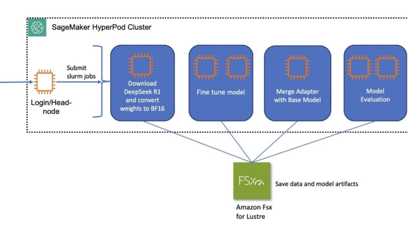
Vishnu Elangovan is a Worldwide Generative AI Solution Architect with over seven years of experience in Applied AI/ML. He holds a master’s degree in Data Science and specializes in building scalable artificial intelligence solutions. He loves building and tinkering with scalable AI/ML solutions and considers himself a lifelong learner. Outside his professional pursuits, he enjoys traveling, participating in sports, and exploring new problems to solve.

Keerthi Konjety is a Specialist Solutions Architect for Amazon Q Developer, with over 3.5 years of experience in Data Engineering, ML and AI. Her expertise lies in enabling developer productivity for AWS customers. Outside work, she enjoys photography and tech content creation.

Read More