Building a custom text-to-SQL agent using Amazon Bedrock and Converse API

Building a custom text-to-SQL agent using Amazon Bedrock and Converse API

Developing robust text-to-SQL capabilities is a critical challenge in the field of natural language processing (NLP) and database management. The complexity of NLP and database management increases in this field, particularly while dealing with complex queries and database structures. In this post, we introduce a straightforward but powerful solution with accompanying code to text-to-SQL using a custom agent implementation along with Amazon Bedrock and Converse API.

The ability to translate natural language queries into SQL statements is a game-changer for businesses and organizations because users can now interact with databases in a more intuitive and accessible manner. However, the complexity of database schemas, relationships between tables, and the nuances of natural language can often lead to inaccurate or incomplete SQL queries. This not only compromises the integrity of the data but also hinders the overall user experience. Through a straightforward yet powerful architecture, the agent can understand your query, develop a plan of execution, create SQL statements, self-correct if there is a SQL error, and learn from its execution to improve in the future. Overtime, the agent can develop a cohesive understanding of what to do and what not to do to efficiently answer queries from users.

Solution overview

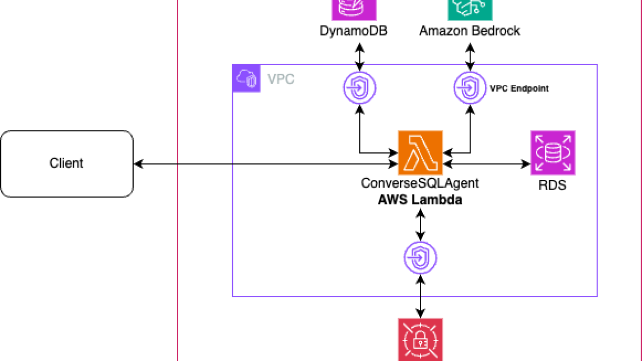
The solution is composed of an AWS Lambda function that contains the logic of the agent that communicates with Amazon DynamoDB for long-term memory retention, calls Anthropic’s Claude Sonnet in Amazon Bedrock through Converse API, uses AWS Secrets Manager to retrieve database connection details and credentials, and Amazon Relational Database Service (Amazon RDS) that contains an example Postgres database called HR Database. The Lambda function is connected to a virtual private cloud (VPC) and communicates with DynamoDB, Amazon Bedrock, and Secrets Manager through AWS PrivateLink VPC endpoints so that the Lambda can communicate with the RDS database while keeping traffic private through AWS networking.

In the demo, you can interact with the agent through the Lambda function. You can provide it a natural language query, such as “How many employees are there in each department in each region?” or “What is the employee mix by gender in each region”. The following is the solution architecture.

Solution Diagram

A custom agent build using Converse API

Converse API is provided by Amazon Bedrock for you to be able to create conversational applications. It enables powerful features such as tool use. Tool use is the ability for a large language model (LLM) to choose from a list of tools, such as running SQL queries against a database, and decide which tool to use depending on the context of the conversation. Using Converse API also means you can maintain a series of messages between User and Assistant roles to carry out a chat with an LLM such as Anthropic’s Claude 3.5 Sonnet. In this post, a custom agent called ConverseSQLAgent was created specifically for long-running agent executions and to follow a plan of execution.

The Agent loop: Agent planning, self-correction, and long-term learning

The agent contains several key features: planning and carry-over, execution and tool use, SQLAlchemy and self-correction, reflection and long-term learning using memory.

Planning and carry-over

The first step that the agent takes is to create a plan of execution to perform the text-to-SQL task. It first thinks through what the user is asking and develops a plan on how it will fulfill the request of the user. This behavior is controlled using a system prompt, which defines how the agent should behave. After the agent thinks through what it should do, it outputs the plan.

One of the challenges with long-running agent execution is that sometimes the agent will forget the plan that it was supposed to execute as the context becomes longer and longer as it conducts its steps. One of the primary ways to deal with this is by “carrying over the initial plan by injecting it back into a section in the system prompt. The system prompt is part of every converse API call, and it improves the ability of the agent to follow its plan. Because the agent may revise its plan as it progresses through the execution, the plan in the system prompt is updated as new plans emerge. Refer to the following figure on how the carry over works.

Process Flow

Execution and tool use

After the plan has been created, the agent will execute its plan one step at a time. It might decide to call on one or more tools it has access to. With Converse API, you can pass in a toolConfig that contains the toolSpec for each tool it has access to. The toolSpec defines what the tool is, a description of the tool, and the parameters that the tool requires. When the LLM decides to use a tool, it outputs a tool use block as part of its response. The application, in this case the Lambda code, needs to identify that tool use block, execute the corresponding tool, append the tool result response to the message list, and call the Converse API again. As shown at (a) in the following figure, you can add tools for the LLM to choose from by adding in a toolConfig along with toolSpecs. Part (b) shows that in the implementation of ConverseSQLAgent, tool groups contain a collection of tools, and each tool contains the toolSpec and the callable function. The tool groups are added to the agent, which in turn adds it to the Converse API call. Tool group instructions are additional instructions on how to use the tool group that get injected into the system prompt. Although you can add descriptions to each individual tool, having tool group–wide instructions enable more effective usage of the group.

Converse API processing Tools

SQLAlchemy and self-correction

The SQL tool group (these tools are part of the demo code provided), as shown in the preceding figure, is implemented using SQLAlchemy, which is a Python SQL toolkit you can use to interface with different databases without having to worry about database-specific SQL syntax. You can connect to Postgres, MySQL, and more without having to change your code every time.

In this post, there is an InvokeSQLQuery tool that allows the agent to execute arbitrary SQL statements. Although almost all database specific tasks, such as looking up schemas and tables, can be accomplished through InvokeSQLQuery, it’s better to provide SQLAlchemy implementations for specific tasks, such as GetDatabaseSchemas, which gets every schema in the database, greatly reducing the time it takes for the agent to generate the correct query. Think of it as giving the agent a shortcut to getting the information it needs. The agents can make errors in querying the database through the InvokeSQLQuery tool. The InvokeSQLQuery tool will respond with the error that it encountered back to the agent, and the agent can perform self-correction to correct the query. This flow is shown in the following diagram.

Agent Flow

Reflection and long-term learning using memory

Although self-correction is an important feature of the agent, the agent must be able to learn through its mistakes to avoid the same mistake in the future. Otherwise, the agent will continue to make the mistake, greatly reducing effectiveness and efficiency. The agent maintains a hierarchical memory structure, as shown in the following figure. The agent decides how to structure its memory. Here is an example on how it may structure it.

Memory Management

The agent can reflect on its execution, learn best practices and error avoidance, and save it into long-term memory. Long-term memory is implemented through a hierarchical memory structure with Amazon DynamoDB. The agent maintains a main memory that has pointers to other memories it has. Each memory is represented as a record in a DynamoDB table. As the agent learns through its execution and encounters errors, it can update its main memory and create new memories by maintaining an index of memories in the main memory. It can then tap onto this memory in the future to avoid errors and even improve the efficiency of queries by caching facts.

Prerequisites

Before you get started, make sure you have the following prerequisites:

Deploy the solution

The full code and instructions are available in GitHub in the Readme file.

  1. Clone the code to your working environment:

git clone https://github.com/aws-samples/aws-field-samples.git

  1. Move to ConverseSqlAgent folder
  2. Follow the steps in the Readme file in the GitHub repo

Cleanup

To dispose of the stack afterwards, invoke the following command:

cdk destroy

Conclusion

The development of robust text-to-SQL capabilities is a critical challenge in natural language processing and database management. Although current approaches have made progress, there remains room for improvement, particularly with complex queries and database structures. The introduction of the ConverseSQLAgent, a custom agent implementation using Amazon Bedrock and Converse API, presents a promising solution to this problem. The agent’s architecture, featuring planning and carry-over, execution and tool use, self-correction through SQLAlchemy, and reflection-based long-term learning, demonstrates its ability to understand natural language queries, develop and execute SQL plans, and continually improve its capabilities. As businesses seek more intuitive ways to access and manage data, solutions such as the ConverseSQLAgent hold the potential to bridge the gap between natural language and structured database queries, unlocking new levels of productivity and data-driven decision-making. To dive deeper and learn more about generative AI, check out these additional resources:


About the authors

Pavan KumarPavan Kumar is a Solutions Architect at Amazon Web Services (AWS), helping customers design robust, scalable solutions on the cloud across multiple industries. With a background in enterprise architecture and software development, Pavan has contributed to creating solutions to handle API security, API management, microservices, and geospatial information system use cases for his customers. He is passionate about learning new technologies and solving, automating, and simplifying customer problems using these solutions.

Abdullah SiddiquiAbdullah Siddiqui is a Partner Sales Solutions Architect at Amazon Web Services (AWS) based out of Toronto. He helps AWS Partners and customers build solutions using AWS services and specializes in resilience and migrations. In his spare time, he enjoys spending time with his family and traveling.

Parag SrivastavaParag Srivastava is a Solutions Architect at Amazon Web Services (AWS), helping enterprise customers with successful cloud adoption and migration. During his professional career, he has been extensively involved in complex digital transformation projects. He is also passionate about building innovative solutions around geospatial aspects of addresses.

Read More

Accelerate threat modeling with generative AI

Accelerate threat modeling with generative AI

In this post, we explore how generative AI can revolutionize threat modeling practices by automating vulnerability identification, generating comprehensive attack scenarios, and providing contextual mitigation strategies. Unlike previous automation attempts that struggled with the creative and contextual aspects of threat analysis, generative AI overcomes these limitations through its ability to understand complex system relationships, reason about novel attack vectors, and adapt to unique architectural patterns. Where traditional automation tools relied on rigid rule sets and predefined templates, AI models can now interpret nuanced system designs, infer security implications across components, and generate threat scenarios that human analysts might overlook, making effective automated threat modeling a practical reality.

Threat modeling and why it matters

Threat modeling is a structured approach to identifying, quantifying, and addressing security risks associated with an application or system. It involves analyzing the architecture from an attacker’s perspective to discover potential vulnerabilities, determine their impact, and implement appropriate mitigations. Effective threat modeling examines data flows, trust boundaries, and potential attack vectors to create a comprehensive security strategy tailored to the specific system.

In a shift-left approach to security, threat modeling serves as a critical early intervention. By implementing threat modeling during the design phase—before a single line of code is written—organizations can identify and address potential vulnerabilities at their inception point. The following diagram illustrates this workflow.

Threat modeling in shift-left

This proactive strategy significantly reduces the accumulation of security debt and transforms security from a bottleneck into an enabler of innovation. When security considerations are integrated from the beginning, teams can implement appropriate controls throughout the development lifecycle, resulting in more resilient systems built from the ground up.

Despite these clear benefits, threat modeling remains underutilized in the software development industry. This limited adoption stems from several significant challenges inherent to traditional threat modeling approaches:

  • Time requirements – The process takes 1–8 days to complete, with multiple iterations needed for full coverage. This conflicts with tight development timelines in modern software environments.
  • Inconsistent assessment – Threat modeling suffers from subjectivity. Security experts often vary in their threat identification and risk level assignments, creating inconsistencies across projects and teams.
  • Scaling limitations – Manual threat modeling can’t effectively address modern system complexity. The growth of microservices, cloud deployments, and system dependencies outpaces security teams’ capacity to identify vulnerabilities.

How generative AI can help

Generative AI has revolutionized threat modeling by automating traditionally complex analytical tasks that required human judgment, reasoning, and expertise. Generative AI brings powerful capabilities to threat modeling, combining natural language processing with visual analysis to simultaneously evaluate system architectures, diagrams, and documentation. Drawing from extensive security databases like MITRE ATT&CK and OWASP, these models can quickly identify potential vulnerabilities across complex systems. This dual capability of processing both text and visuals while referencing comprehensive security frameworks enables faster, more thorough threat assessments than traditional manual methods.

Our solution, Threat Designer, uses enterprise-grade foundation models (FMs) available in Amazon Bedrock to transform threat modeling. Using Anthropic’s Claude Sonnet 3.7 advanced multimodal capabilities, we create comprehensive threat assessments at scale. You can also use other available models from the model catalog or use your own fine-tuned model, giving you maximum flexibility to use pre-trained expertise or custom-tailored capabilities specific to your security domain and organizational requirements. This adaptability makes sure your threat modeling solution delivers precise insights aligned with your unique security posture.

Solution overview

Threat Designer is a user-friendly web application that makes advanced threat modeling accessible to development and security teams. Threat Designer uses large language models (LLMs) to streamline the threat modeling process and identify vulnerabilities with minimal human effort.

Key features include:

  • Architecture diagram analysis – Users can submit system architecture diagrams, which the application processes using multimodal AI capabilities to understand system components and relationships
  • Interactive threat catalog – The system generates a comprehensive catalog of potential threats that users can explore, filter, and refine through an intuitive interface
  • Iterative refinement – With the replay functionality, teams can rerun the threat modeling process with design improvements or modifications, and see how changes impact the system’s security posture
  • Standardized exports – Results can be exported in PDF or DOCX formats, facilitating integration with existing security documentation and compliance processes
  • Serverless architecture – The solution runs on a cloud-based serverless infrastructure, alleviating the need for dedicated servers and providing automatic scaling based on demand

The following diagram illustrates the Threat Designer architecture.

Architecture diagram

The solution is built on a serverless stack, using AWS managed services for automatic scaling, high availability, and cost-efficiency. The solution is composed of the following core components:

  • FrontendAWS Amplify hosts a ReactJS application built with the Cloudscape design system, providing the UI
  • AuthenticationAmazon Cognito manages the user pool, handling authentication flows and securing access to application resources
  • API layerAmazon API Gateway serves as the communication hub, providing proxy integration between frontend and backend services with request routing and authorization
  • Data storage – We use the following services for storage:
    • Two Amazon DynamoDB tables:
      • The agent execution state table maintains processing state
      • The threat catalog table stores identified threats and vulnerabilities
    • An Amazon Simple Storage Service (Amazon S3) architecture bucket stores system diagrams and artifacts
  • Generative AI – Amazon Bedrock provides the FM for threat modeling, analyzing architecture diagrams and identifying potential vulnerabilities
  • Backend service – An AWS Lambda function contains the REST interface business logic, built using Powertools for AWS Lambda (Python)
  • Agent service – Hosted on a Lambda function, the agent service works asynchronously to manage threat analysis workflows, processing diagrams and maintaining execution state in DynamoDB

Agent service workflow

The agent service is built on LangGraph by LangChain, with which we can orchestrate complex workflows through a graph-based structure. This approach incorporates two key design patterns:

  • Separation of concerns – The threat modeling process is decomposed into discrete, specialized steps that can be executed independently and iteratively. Each node in the graph represents a specific function, such as image processing, asset identification, data flow analysis, or threat enumeration.
  • Structured output – Each component in the workflow produces standardized, well-defined outputs that serve as inputs to subsequent steps, providing consistency and facilitating downstream integrations for consistent representation.

The agent workflow follows a directed graph where processing begins at the Start node and proceeds through several specialized stages, as illustrated in the following diagram.

Agent anatomy

The workflow includes the following nodes:

  • Image processing – The Image processing node processes the architecture diagram image and converts it in the appropriate format for the LLM to consume
  • Assets – This information, along with textual descriptions, feeds into the Assets node, which identifies and catalogs system components
  • Flows – The workflow then progresses to the Flows node, mapping data movements and trust boundaries between components
  • Threats – Lastly, the Threats node uses this information to identify potential vulnerabilities and attack vectors

A critical innovation in our agent architecture is the adaptive iteration mechanism implemented through conditional edges in the graph. This feature addresses one of the fundamental challenges in LLM-based threat modeling: controlling the comprehensiveness and depth of the analysis.

The conditional edge after the Threats node enables two powerful operational modes:

  • User-controlled iteration – In this mode, the user specifies the number of iterations the agent should perform. With each pass through the loop, the agent enriches the threat catalog by analyzing edge cases that might have been overlooked in previous iterations. This approach gives security professionals direct control over the thoroughness of the analysis.
  • Autonomous gap analysis – In fully agentic mode, a specialized gap analysis component evaluates the current threat catalog. This component identifies potential blind spots or underdeveloped areas in the threat model and triggers additional iterations until it determines the threat catalog is sufficiently comprehensive. The agent essentially performs its own quality assurance, continuously refining its output until it meets predefined completeness criteria.

Prerequisites

Before you deploy Threat Designer, make sure you have the required prerequisites in place. For more information, refer to the GitHub repo.

Get started with Threat Designer

To start using Threat Designer, follow the step-by-step deployment instructions from the project’s README available in GitHub. After you deploy the solution, you’re ready to create your first threat model. Log in and complete the following steps:

  1. Choose Submit threat model to initiate a new threat model.
  2. Complete the submission form with your system details:
    • Required fields: Provide a title and architecture diagram image.
    • Recommended fields: Provide a solution description and assumptions (these significantly improve the quality of the threat model).
  3. Configure analysis parameters:
    • Choose your iteration mode:
      1. Auto (default): The agent intelligently determines when the threat catalog is comprehensive.
      2. Manual: Specify up to 15 iterations for more control.
    • Configure your reasoning boost to specify how much time the model spends on analysis (available when using Anthropic’s Claude Sonnet 3.7).
  4. Choose Start threat modeling to launch the analysis.

Wizard

You can monitor progress through the intuitive interface, which displays each execution step in real time. The complete analysis typically takes between 5–15 minutes, depending on system complexity and selected parameters.

Workflow

When the analysis is complete, you will have access to a comprehensive threat model that you can explore, refine, and export.

Threat modeling results

Clean up

To avoid incurring future charges, delete the solution by running the ./destroy.sh script. Refer to the README for more details.

Conclusion

In this post, we demonstrated how generative AI transforms threat modeling from an exclusive, expert-driven process into an accessible security practice for all development teams. By using FMs through our Threat Designer solution, we’ve democratized sophisticated security analysis, enabling organizations to identify vulnerabilities earlier and more consistently. This AI-powered approach removes the traditional barriers of time, expertise, and scalability, making shift-left security a practical reality rather than just an aspiration—ultimately building more resilient systems without sacrificing development velocity.

Deploy Threat Designer following the README instructions, upload your architecture diagram, and quickly receive AI-generated security insights. This streamlined approach helps you integrate proactive security measures into your development process without compromising speed or innovation—making comprehensive threat modeling accessible to teams of different sizes.


About the Authors

Edvin HallvaxhiuEdvin Hallvaxhiu is a senior security architect at Amazon Web Services, specialized in cybersecurity and automation. He helps customers design secure, compliant cloud solutions.

Sindi CaliSindi Cali is a consultant with AWS Professional Services. She supports customers in building data-driven applications in AWS.

Aditi GuptaAditi Gupta is a Senior Global Engagement Manager at AWS ProServe. She specializes in delivering impactful Big Data and AI/ML solutions that enable AWS customers to maximize their business value through data utilization.

Rahul ShauryaRahul Shaurya is a Principal Data Architect at Amazon Web Services. He helps and works closely with customers building data platforms and analytical applications on AWS.

Read More

Plug and Play: Build a G-Assist Plug-In Today

Plug and Play: Build a G-Assist Plug-In Today

Project G-Assist — available through the NVIDIA App — is an experimental AI assistant that helps tune, control and optimize NVIDIA GeForce RTX systems.

NVIDIA’s Plug and Play: Project G-Assist Plug-In Hackathon — running virtually through Wednesday, July 16 — invites the community to explore AI and build custom G-Assist plug-ins for a chance to win prizes and be featured on NVIDIA social media channels.

G-Assist allows users to control their RTX GPU and other system settings using natural language, thanks to a small language model that runs on device. It can be used from the NVIDIA Overlay in the NVIDIA App without needing to tab out or switch programs. Users can expand its capabilities via plug-ins and even connect it to agentic frameworks such as Langflow.

Below, find popular G-Assist plug-ins, hackathon details and tips to get started.

Plug-In and Win

Join the hackathon by registering and checking out the curated technical resources.

G-Assist plug-ins can be built in several ways, including with Python for rapid development, with C++ for performance-critical apps and with custom system interactions for hardware and operating system automation.

For those that prefer vibe coding, the G-Assist Plug-In Builder — a ChatGPT-based app that allows no-code or low-code development with natural language commands — makes it easy for enthusiasts to start creating plug-ins.

To submit an entry, participants must provide a GitHub repository, including source code file (plugin.py), requirements.txt, manifest.json, config.json (if applicable), a plug-in executable file and READme code.

Then, submit a video — between 30 seconds and two minutes — showcasing the plug-in in action.

Finally, hackathoners must promote their plug-in using #AIonRTXHackathon on a social media channel: Instagram, TikTok or X. Submit projects via this form by Wednesday, July 16.

Judges will assess plug-ins based on three main criteria: 1) innovation and creativity, 2) technical execution and integration, reviewing technical depth, G-Assist integration and scalability, and 3) usability and community impact, aka how easy it is to use the plug-in.

Winners will be selected on Wednesday, Aug. 20. First place will receive a GeForce RTX 5090 laptop, second place a GeForce RTX 5080 GPU and third a GeForce RTX 5070 GPU. These top three will also be featured on NVIDIA’s social media channels, get the opportunity to meet the NVIDIA G-Assist team and earn an NVIDIA Deep Learning Institute self-paced course credit.

Project G-Assist requires a GeForce RTX 50, 40 or 30 Series Desktop GPU with at least 12GB of VRAM, Windows 11 or 10 operating system, a compatible CPU (Intel Pentium G Series, Core i3, i5, i7 or higher; AMD FX, Ryzen 3, 5, 7, 9, Threadripper or higher), specific disk space requirements and a recent GeForce Game Ready Driver or NVIDIA Studio Driver.

Plug-In(spiration)

Explore open-source plug-in samples available on GitHub, which showcase the diverse ways on-device AI can enhance PC and gaming workflows.

Popular plug-ins include:

  • Google Gemini: Enables search-based queries using Google Search integration and large language model-based queries using Gemini capabilities in real time without needing to switch programs from the convenience of the NVIDIA App Overlay.
  • Discord: Enables users to easily share game highlights or messages directly to Discord servers without disrupting gameplay.
  • IFTTT: Lets users create automations across hundreds of compatible endpoints to trigger IoT routines — such as adjusting room lights and smart shades, or pushing the latest gaming news to a mobile device.
  • Spotify: Lets users control Spotify using simple voice commands or the G-Assist interface to play favorite tracks and manage playlists.
  • Twitch: Checks if any Twitch streamer is currently live and can access detailed stream information such as titles, games, view counts and more.

Get G-Assist(ance) 

Join the NVIDIA Developer Discord channel to collaborate, share creations and gain support from fellow AI enthusiasts and NVIDIA staff.

Save the date for NVIDIA’s How to Build a G-Assist Plug-In webinar on Wednesday, July 9, from 10-11 a.m. PT, to learn more about Project G-Assist capabilities, discover the fundamentals of building, testing and deploying Project G-Assist plug-ins, and participate in a live Q&A session.

Explore NVIDIA’s GitHub repository, which provides everything needed to get started developing with G-Assist, including sample plug-ins, step-by-step instructions and documentation for building custom functionalities.

Learn more about the ChatGPT Plug-In Builder to transform ideas into functional G-Assist plug-ins with minimal coding. The tool uses OpenAI’s custom GPT builder to generate plug-in code and streamline the development process.

NVIDIA’s technical blog walks through the architecture of a G-Assist plug-in, using a Twitch integration as an example. Discover how plug-ins work, how they communicate with G-Assist and how to build them from scratch.

Each week, the RTX AI Garage blog series features community-driven AI innovations and content for those looking to learn more about NVIDIA NIM microservices and AI Blueprints, as well as building AI agents, creative workflows, digital humans, productivity apps and more on AI PCs and workstations. 

Plug in to NVIDIA AI PC on Facebook, Instagram, TikTok and X — and stay informed by subscribing to the RTX AI PC newsletter.

Follow NVIDIA Workstation on LinkedIn and X

See notice regarding software product information.

Read More

Breaking bonds, breaking ground: Advancing the accuracy of computational chemistry with deep learning

Breaking bonds, breaking ground: Advancing the accuracy of computational chemistry with deep learning

Alt text: A dark blue, wavy surface with multiple colorful spheres placed on it. The spheres are in various colors including red, green, blue, yellow, purple, and orange. Each sphere is surrounded by small white particles that appear to be floating around them. The background is a gradient of dark teal to black.

We are excited to share our first big milestone in solving a grand challenge that has hampered the predictive power of computational chemistry, biochemistry, and materials science for decades. By using a scalable deep-learning approach and generating an unprecedented quantity of diverse, highly accurate data, we have achieved a breakthrough in the accuracy of density functional theory (DFT), the workhorse method that thousands of scientists use every year to simulate matter at the atomistic level. Within the region of chemical space represented in our large training dataset, our model reaches the accuracy required to reliably predict experimental outcomes, as assessed on the well-known benchmark dataset W4-17 (opens in new tab). This removes a fundamental barrier to shifting the balance of molecule and material design from being driven by laboratory experiments to being driven by computational simulations. The implications for accelerating scientific discovery are far reaching, spanning applications from drugs to batteries and green fertilizers.

What is DFT?

Molecules and materials are made of atoms, which are held together by their electrons. These electrons act as a glue, determining the stability and properties of the chemical structure. Accurately computing the strength and properties of the electron glue is essential for predicting whether a chemical reaction will proceed, whether a candidate drug molecule will bind to its target protein, whether a material is suitable for carbon capture, or if a flow battery can be optimized for renewable energy storage. Unfortunately, a brute-force approach amounts to solving the many-electron Schrödinger equation, which requires computation that scales exponentially with the number of electrons. Considering that an atom has dozens of electrons, and that molecules and materials have large numbers of atoms, we could easily end up waiting the age of the universe to complete our computation unless we restrict our attention to small systems with only a few atoms.

DFT, introduced by Walter Kohn and collaborators in 1964-1965, was a true scientific breakthrough, earning Kohn the Nobel Prize in Chemistry in 1998. DFT provides an extraordinary reduction in the computational cost of calculating the electron glue in an exact manner, from exponential to cubic, making it possible to perform calculations of practical value within seconds to hours.

What is the grand challenge in DFT? 

But there is a catch: the exact reformulation has a small but crucial term—the exchange-correlation (XC) functional—which Kohn proved is universal (i.e., the same for all molecules and materials), but for which no explicit expression is known. For 60 years, people have designed practical approximations for the XC functional. The magazine Science dubbed the gold rush to design better XC models the “pursuit of the Divine Functional (opens in new tab)”. With time, these approximations have grown into a zoo of hundreds of different XC functionals from which users must choose, often using experimental data as a guide. Owing to the uniquely favorable computational cost of DFT, existing functionals have enabled scientists to gain extremely useful insight into a huge variety of chemical problems. However, the limited accuracy and scope of current XC functionals mean that DFT is still mostly used to interpret experimental results rather than predict them.

Why is it important to increase the accuracy of DFT? 

We can contrast the present state of computational chemistry with the state of aircraft engineering and design. Thanks to predictive simulations, aeronautical engineers no longer need to build and test thousands of prototypes to identify one viable design. However, this is exactly what we currently must do in molecular and materials sciences. We send thousands of potential candidates to the lab, because the accuracy of the computational methods is not sufficient to predict the experiments. To make a significant shift in the balance from laboratory to in silico experiments, we need to remove the fundamental bottleneck of the insufficient accuracy of present XC functionals. This amounts to bringing the error of DFT calculations with respect to experiments within chemical accuracy, which is around 1 kcal/mol for most chemical processes. Present approximations typically have errors that are 3 to 30 times larger.

How can AI make a difference? 

AI can transform how we model molecules and materials with DFT by learning the XC functional directly from highly accurate data. The goal is to learn how the XC functional captures the complex relationship between its input, the electron density, and its output, the XC energy. You can think of the density like a glue, with regions of space where there is a lot of it and other regions with less of it. Traditionally, researchers have built XC functional approximations using the concept of the so-called Jacob’s ladder: a hierarchy of increasingly complex, hand-designed descriptors of the electron density. Including density descriptors from higher rungs of this ladder aims to improve accuracy, but it comes at the price of increased computational cost. Even the few attempts that use machine learning have stayed within this traditional paradigm, thereby taking an approach that is akin to what people were doing in computer vision and speech recognition before the deep-learning era. Progress toward better accuracy has stagnated for at least two decades with this approach. 

Our project is driven by the intuition that a true deep learning approach—where relevant representations of the electron density are learned directly from data in a computationally scalable way—has the potential to revolutionize the accuracy of DFT, much like deep learning has transformed other fields. A significant challenge with going down this path, however, is that feature or representation learning is very data-hungry, and there is very little data around—too little to test this hypothesis reliably.

What have we done in this milestone?

The first step was generating data—a lot of it. This posed a major challenge, since the data must come from accurate solutions of the many-electron Schrödinger equation, which is precisely the prohibitively expensive problem that DFT is designed to replace. Fortunately, decades of progress in the scientific community have led to smarter, more efficient variants of brute-force methods, making it possible to compute reference data for small molecules at experimental accuracy. While these high-accuracy methods, also referred to as wavefunction methods, are far too costly for routine use in applications, we made a deliberate investment in them for this project. The reason? The upfront cost of generating high-quality training data is offset by the long-term benefit of enabling vast numbers of industrially relevant applications with cost effective DFT using the trained XC functional. Crucially, we rely on the ability of DFT—and our learned XC functional—to generalize from high-accuracy data for small systems to larger, more complex molecules. 

There are many different high-accuracy wavefunction methods, each tailored to different regions of chemical space. However, their use at scale is not well established, as they require extensive expertise—small methodological choices can significantly affect accuracy at the level that we target. We therefore joined forces with Prof. Amir Karton (opens in new tab) from the University of New England, Australia, a world-leading expert who developed widely recognized benchmark datasets for a fundamental thermochemical property: atomization energy—the energy required to break all bonds in a molecule and separate it into individual atoms. To create a training dataset of atomization energies at unprecedented scale, our team at Microsoft built a scalable pipeline to produce highly diverse molecular structures. Using these structures and substantial Azure compute resources via Microsoft’s Accelerating Foundation Models Research program (opens in new tab), Prof. Karton applied a high-accuracy wavefunction method to compute the corresponding energy labels. The result is a dataset (opens in new tab) two orders of magnitude larger than previous efforts. We are releasing a large part of this dataset (opens in new tab) to the scientific community.

Data generation was only half of the challenge. We also needed to design a dedicated deep-learning architecture for the XC functional—one that is both computationally scalable and capable of learning meaningful representations from electron densities to accurately predict the XC energy. Our team of machine learning specialists, assisted by DFT experts, introduced a series of innovations that solve these and other challenges inherent to this complex learning problem. The result is Skala, an XC functional that generalizes to unseen molecules, reaching the accuracy needed to predict experiments. This demonstrates for the first time that deep learning can truly disrupt DFT: reaching experimental accuracy does not require the computationally expensive hand-designed features of Jacob’s ladder. Instead, we can retain the original computational complexity of DFT while allowing the XC functional to learn how to extract meaningful features and predict accurate energies.

We compare the accuracy of Skala against the best existing functionals of varying computational cost. The prediction errors are evaluated on two well-known public benchmark datasets: the W4-17 dataset for atomization energies (y axis, mean absolute error) and the GMTKN55 dataset for general main-group chemistry (x axis, weighted total mean absolute deviation, or WTMAD-2 for short). Skala achieves near
We compare the accuracy of Skala against the best existing functionals of varying computational cost. The prediction errors are evaluated on two well-known public benchmark datasets: the W4-17 dataset for atomization energies (y axis, mean absolute error) and the GMTKN55 dataset for general main-group chemistry (x axis, weighted total mean absolute deviation, or WTMAD-2 for short). Skala achieves near “chemical accuracy” (1 kcal/mol) on atomization energies. This is the accuracy required for predictive modeling of laboratory experiments, which, to date, no existing functional has reached. Skala works especially well on the “single reference” subset of this dataset, reaching a groundbreaking 0.85 kcal/mol. On the GMTKN55 dataset, Skala shows competitive accuracy to the best-performing hybrid functionals, at a lower cost.

Skala is a new density functional for the exchange-correlation energy that employs meta-GGA ingredients plus D3 dispersion and machine-learned nonlocal features of the electron density. Some exact constraints were imposed, and some others “emerge” from the fitting to about 150,000 accurate energy differences for sp molecules and atoms. Skala achieves high, hybrid-like accuracy on a large and diverse data set of properties of main group molecules, which has no overlap with its training set. The computational cost of Skala is higher than that of the r2SCAN meta-GGA for small molecules, but about the same for systems with 1,000 or more occupied orbitals. Its cost seems to be only 10% of the cost of standard hybrids and 1% of the cost of local hybrids. Developed by a Microsoft team of density functional theorists and deep-learning experts, Skala could be the first machine-learned density functional to compete with existing functionals for wide use in computational chemistry, and a sign of things to come in that and related fields. Skala learned from big data and was taught by insightful human scientists.”

— John P. Perdew, Professor of Physics, School of Science and Engineering, Tulane University

This first milestone was achieved for a challenging property in a specific region of chemical space—atomization energies of main group molecules—for which we generated our initial large batch of high-accuracy training data. Building on this foundation, we have started to expand our training dataset to cover a broader range of general chemistry, using our scalable in-house data generation pipeline. With the first small batch of training data beyond atomization energies, we have already extended the accuracy of our model, making it competitive with the best existing XC functionals across a wider spectrum of main group chemistry. This motivates us to continue growing our high-accuracy data generation campaign, engaging with external experts such as Prof. Amir Karton, who noted, “After years of benchmarking DFT methods against experimental accuracy, this is the first time I’ve witnessed such an unprecedented leap in the accuracy–cost trade-off. It is genuinely exciting to see how the creation of our new dataset has enabled these groundbreaking results — opening up a path for transformative advances across chemical, biochemical, and materials research.”

Advancing computational chemistry together

We are excited to work closely with the global computational chemistry community to accelerate progress for all and look forward to openly releasing our first XC functional in the near future. 

Density Functional Theory (DFT) and related technologies are a core Digital Chemistry technology supporting advancements in Merck’s diverse Life Science, Healthcare and Electronics businesses. However, the limitations of traditional DFT methods, which have persisted for the last 50 years, have hindered its full potential. Microsoft Research’s innovative approach to integrating deep learning represents a substantial leap, enhancing its accuracy, robustness, and scalability. We are looking forward to exploring how this can advance Digital Chemistry workflows and unlock new possibilities for the future, aligning with our commitment to developing advanced algorithms and technologies that propel scientific innovation at Merck.”

— Jan Gerit Brandenburg – Director for Digital Chemistry at Merck 

We are entering a golden age for predictive and realistic simulations: very accurate electronic-structure calculations provide vast amounts of consistent data that can be used to train novel machine-learning architectures, delivering the holy grail of precision and computational efficiency.”

— Professor Nicola Marzari, Chair of Theory and Simulation of Materials, EPFL and PSI

We believe that our new functional can help unlock new opportunities for businesses and are eager to work together on real-world applications. Today, we are delighted to launch the DFT Research Early Access Program (DFT REAP) and welcome Flagship Pioneering as the first participant. This program is for companies and research labs to collaborate with us to accelerate innovation across many industries. To find out more about how to join this program please visit: https://aka.ms/DFT-REAP (opens in new tab) 

“Microsoft’s effort to enhance the predictive power of computational chemistry reflects a bold but thoughtful step toward a simulation-first future. At Flagship, we believe that openly shared, foundational advances in science – like this leap forward in DFT accuracy – can serve as powerful enablers of innovation. These next-generation tools promise to accelerate discovery across a wide range of sectors, from therapeutics to materials science, by helping researchers navigate chemical and biological space with far greater precision and speed.”

Junaid Bajwa, M.D., Senior Partner at Flagship Pioneering and Science Partner at Pioneering Intelligence

By making our work available to the scientific community, we hope to enable widespread testing and gather valuable feedback that will guide future improvements. For the first time, deep learning offers a clear and computationally scalable path to building an accurate, efficient, and broadly applicable model of the universal XC functional—one that could transform the computational design of molecules and materials.

Acknowledgement

This work is the product of a highly collaborative and interdisciplinary effort led by Microsoft Research AI for Science, in partnership with colleagues from Microsoft Research Accelerator, Microsoft Quantum and the University of New England. The full author list includes Giulia Luise, Chin-Wei Huang, Thijs Vogels, Derk P. Kooi, Sebastian Ehlert, Stephanie Lanius, Klaas J. H. Giesbertz, Amir Karton, Deniz Gunceler, Megan Stanley, Wessel P. Bruinsma, Victor Garcia Satorras, Marwin Segler, Kenji Takeda, Lin Huang, Xinran Wei, José Garrido Torres, Albert Katbashev, Bálint Máté, Sékou-Oumar Kaba, Roberto Sordillo, Yingrong Chen, David B. Williams-Young, Christopher M. Bishop, Jan Hermann, Rianne van den Berg and Paola Gori Giorgi

The post Breaking bonds, breaking ground: Advancing the accuracy of computational chemistry with deep learning appeared first on Microsoft Research.

Read More

DeepNVMe: Affordable I/O scaling for Deep Learning Applications

DeepNVMe: Affordable I/O scaling for Deep Learning Applications

Introduction

We introduced DeepNVMe in summer 2024 as a suite of optimizations for tackling I/O bottlenecks in Deep Learning (DL). DeepNVMe delivers significant speedups for I/O bound DL workloads by leveraging storage innovations including local NVMe SSDs, NVIDIA Magnum IOTM GPUDirect® Storage (GDS), and Linux Asynchronous I/O (AIO). In this update, we are delighted to announce DeepNVMe improvements on multiple fronts: (i) expanding application coverage to FastPersist model checkpointing and SGLang inference, (ii) I/O performance scaling by upgrading from PCIe Gen4 to Gen5 NVMe SSDs, and (iii) expanding usability to CPU-only environments, offset-based I/O operations, and tensor data type casting. The results reported in this blog are available in DeepSpeed versions >= 0.17.1.

Evaluation environments

Our experiments are conducted on Azure ND-H200-v5 VM. The key software configurations are summarized in the following table.
Software Version
Ubuntu 24.04.2
PyTorch 2.6.0
CUDA 12.6
SGLang 0.4.4.post4

Addressing I/O Bottlenecks of Deep Learning

We used DeepNVMe to develop FastPersist and ZeRO-Inference to target I/O bottlenecks in DL training and inference respectively. Our experiments are conducted using a single VM, in which we combine the available NVMe SSDs into a single RAID-0 (i.e., disk striping) volume to leverage aggregate read and write bandwidths. Since DeepNVMe can offload tensors using CPU bounce buffers (a.k.a., AIO), or NVIDIA GPUDirect Storage (a.k.a., GDS), we report results for both modes.

FastPersist: Faster Model Checkpoint Creation

Although saving model checkpoints to persistent storage is critical in model training, it is also a major bottleneck due to the inefficiencies of existing approaches. We developed FastPersist to address the performance challenges of checkpointing. FastPersist makes checkpointing overheads negligible during training through three key techniques: (i) DeepNVMe, (ii) data parallelism, and (iii) overlapping I/O and computation.

Our goal here is to demonstrate the impact of DeepNVMe in FastPersist using single-process micro-benchmarks (available here), which serialize a model checkpoint state from HBM to local NVMe. We use the popular PyTorch torch.save() as the baseline in our experiments, and integrate FastPersist into torch.save() to simplify adoption and performance comparisons.

Faster Saving of PyTorch Models to local NVMe Storage

We measure the throughput of serializing Phi-3-Mini checkpoint state from HBM to local NVMe storage. The results are summarized in the Figure below. We observe significantly faster checkpointing with FastPersist compared to the baseline. We see speedups of over 20X in the 8xGen5 NVMe settings. We also observe FastPersist scaling with increased NVMe bandwidth of 8xGen5 compared with 4xGen5.

FastPersist provides significantly faster model checkpointing to local NVMe.

ZeRO-Inference: Democratizing Generative AI

ZeRO-Inference is a technology that democratizes access to state-of-the-art models by reducing the GPU costs of model inference. ZeRO-Inference enables inference computations of massive models (hundreds-of-billions of parameters) on as few as one GPU by offloading the model weights to DRAM and NVMe storage. ZeRO-Inference is designed for offline or throughput-oriented inference scenarios. In this blog, we share two updates on ZeRO-Inference. First, we have integrated ZeRO-Inference into SGLang, a state-of-the-art model serving framework. Second, we observed ZeRO-Inference performance scales with the faster NVMe SSDs in the latest Azure SKUs.

Democratizing SGLang through ZeRO-Inference integration

SGLang is a state-of-the-art serving framework for large language models (LLMs) and vision language models (VLMs). Our integration of ZeRO-Inference into SGLang makes SGLang available to budget-constrained users, and offers a cost-reduction option to existing SGLang users. We used SGLang’s offline benchmarking tool to measure the generation throughput of LLAMA3-70B on a single H200 with NVMe offloading (LLAMA3-70B cannot fit in the 141GB VRAM without offloading). The experiment is configured with prompt length of 512, generation length of 32, and batch size of 128. We summarize the results in the figure below for both AIO and GDS offloading.

ZeRO-Inference improves SGLang inference with NVMe offloading to reduce hardware costs.

Scaling HF Transformer Generation with Faster NVMe SSDs

ZeRO-Inference enhances HF Transformer inference with efficient model offloading to DRAM or NVMe. We previously evaluated LLAMA-3-70B generation performance with NVMe offloading on a single GPU and four Gen4 NVMes in an Azure NC_A100_v4 VM. We measured the generation speed for a prompt of 512 tokens, output of 32 tokens, and batch size 96. Since NVMe bandwidth was the main bottleneck, we repeat the experiments on Azure ND-H200-v5 offering Gen5 NVMes. The results summarized in the Figure below show that ZeRO-Inference uses the increased NVMe bandwidths to improve generation speeds. For example, with GDS, generation speed improves from 7 tokens/sec with four Gen4 NVMes to 17 tokens/sec with four Gen5 NVMes, and further to 26 tokens/sec with eight Gen5 NVMes. We observe similar improvements without GDS. These results show that ZeRO-Inference performance can be improved in cost-effective manner by increasing NVMe bandwidths.

ZeRO-Inference leverages available NVMe bandwidth to scale LLAMA-3-70B generation.

I/O performance scaling

We used our ds_io benchmarking tool to demonstrate DeepNVMe proportionally scaling I/O performance with available NVMe bandwidths. This empowers users to accelerate I/O bound DL applications at modest cost using more or faster NVMe SSDs. In our experiments, we measure the achieved read and write bandwidths of 1GB data transfers between HBM and NVMes. We evaluate scaling up NVMes from PCIe Gen4 to Gen5, and scaling out from 4 to 8 SSDs. The SSDs are combined into a single RAID-0 (disk striping) volume. We summarize the results in the Figure below which show that DeepNVMe scales I/O performance on both dimensions. Scaling up from 4xGen4 SSDs to 4xGen5 SSDs improves reads from 10GB/sec to 27GB/sec, and writes from 5GB/sec to 11GB/sec. Scaling out from 4xGen5 to 8xGen5 further improves reads to 48GB/sec, and writes to 26GB/sec.

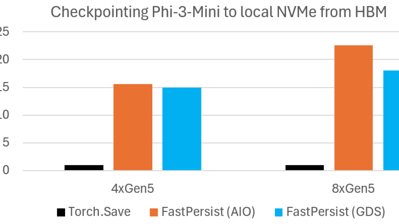
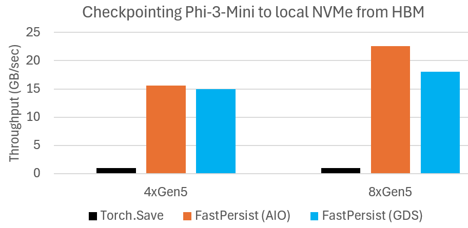
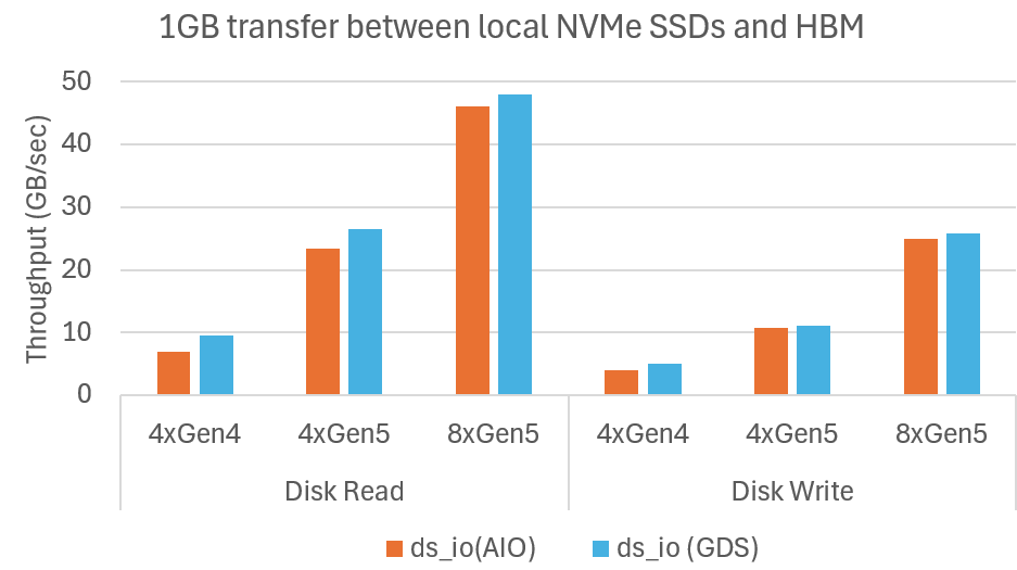
Microbenchmark shows DeepNVMe scales I/O performance with available NVMe bandwidth

Broadening usability

We have increased the usage scenarios of DeepNVMe by removing restrictions regarding hardware environments and I/O operations, as explained below.

CPU-Only environments

Although GPUs (and similar accelerators) dominate DL, CPUs are still used in important machine learning (ML) workloads such as recommendation systems. However, DeepNVMe was previously unusable in CPU-only environments. This was because DeepNVMe relied on torch.pin_memory() for page-locked CPU tensors, whereas torch.pin_memory() does not work in the CPU versions of torch as illustrated below.

>>> import torch
>>> torch.__version__
'2.6.0+cpu'
>>> x = torch.empty(1024).pin_memory()
Traceback (most recent call last):
File "<stdin>", line 1, in <module>
RuntimeError: Cannot access accelerator device when none is available.
>>>

We have made DeepNVMe usable in CPU environments by adding mechanisms for allocating (new_cpu_locked_tensor()) and releasing (free_cpu_locked_tensor()) page-locked CPU tensors. The snippet below illustrates allocating a pinned CPU tensor (x).

>> import torch
>>> torch.__version__
'2.6.0+cpu'
>>> from deepspeed.ops.op_builder import AsyncIOBuilder
>>> h = AsyncIOBuilder().load().aio_handle()
>>> x = h.new_cpu_locked_tensor(1024, torch.Tensor())
>>> x.shape
torch.Size([1024])
>>> x.dtype
torch.float32

Offset-based I/O operations

Previously, DeepNVMe functionality was restricted to reading or writing the entire contents of a file. We have now improved DeepNVMe to read or write a user-specified portion of file content from a given offset. In particular, we have extended the existing read/write APIs to accept a user-specified file offset argument (with default value 0) such as below:

>> from deepspeed.ops.op_builder import AsyncIOBuilder
>>> help(AsyncIOBuilder().load().aio_handle().pread)
Help on method pread in module async_io:

pread(...) method of async_io.aio_handle instance
pread(self: async_io.aio_handle, buffer: torch.Tensor, filename: str, validate: bool, async: bool, file_offset: int = 0) -> int

Tensor data type casting

While developing FastPersist, we needed to manipulate model tensors, typically of floating point data types, in byte format for both performance and convenience of I/O operations. However, we could not find a zero-copy mechanism for casting tensors from arbitrary data types to a byte data type (i.e., torch.uint8), so we decided to create one. This functionality is available via the UtilsBuilder op as demonstrated in the example below. In the example, we cast a torch.bfloat16 tensor into torch.uint8. Note that due to the zero-copy nature of the functionality, bf16_tensor and byte_tensor are aliases.

>>> import torch
>>> from deepspeed.ops.op_builder import UtilsBuilder
>>> util_ops = UtilsBuilder().load()
>>> bf16_tensor = torch.zeros(1024, dtype=torch.bfloat16, device='cuda')
>>> bf16_tensor
tensor([0., 0., 0., ..., 0., 0., 0.], device='cuda:0', dtype=torch.bfloat16)
>>> byte_tensor = util_ops.cast_to_byte_tensor(bf16_tensor)
>>> byte_tensor
tensor([0, 0, 0, ..., 0, 0, 0], device='cuda:0', dtype=torch.uint8)
>>> bf16_tensor += 1.0
>>> bf16_tensor
tensor([1., 1., 1., ..., 1., 1., 1.], device='cuda:0', dtype=torch.bfloat16)
>>> byte_tensor
tensor([128, 63, 128, ..., 63, 128, 63], device='cuda:0',
dtype=torch.uint8)

Summary

This blog post has provided updates on our continued development of DeepNVMe, an I/O optimization technology for accelerating DL applications. We have announced DeepNVMe improvements on multiple aspects, including application coverage, I/O performance scaling, and usability.

Acknowledgements

This blog describes work done by Joe Mayer, Logan Adams, and Olatunji Ruwase of the DeepSpeed team at Microsoft.

Read More