Monthly Archives: July 2025

Although rapid generative AI advancements are revolutionizing organizational natural language processing tasks, developers and data scientists face significant challenges customizing these large models. These hurdles include managing complex workflows, efficiently preparing large datasets for fine-tuning, implementing sophisticated fine-tuning techniques while optimizing computational resources, consistently tracking model performance, and achieving reliable, scalable deployment.The fragmented nature of these tasks often leads to reduced productivity, increased development time, and potential inconsistencies in the model development pipeline. Organizations need a unified, streamlined approach that simplifies the entire process from data preparation to model deployment.

To address these challenges, AWS has expanded Amazon SageMaker with a comprehensive set of data, analytics, and generative AI capabilities. At the heart of this expansion is Amazon SageMaker Unified Studio, a centralized service that serves as a single integrated development environment (IDE). SageMaker Unified Studio streamlines access to familiar tools and functionality from purpose-built AWS analytics and artificial intelligence and machine learning (AI/ML) services, including Amazon EMR, AWS Glue, Amazon Athena, Amazon Redshift, Amazon Bedrock, and Amazon SageMaker AI. With SageMaker Unified Studio, you can discover data through Amazon SageMaker Catalog, access it from Amazon SageMaker Lakehouse, select foundation models (FMs) from Amazon SageMaker JumpStart or build them through JupyterLab, train and fine-tune them with SageMaker AI training infrastructure, and deploy and test models directly within the same environment. SageMaker AI is a fully managed service to build, train, and deploy ML models—including FMs—for different use cases by bringing together a broad set of tools to enable high-performance, low-cost ML. It’s available as a standalone service on the AWS Management Console, or through APIs. Model development capabilities from SageMaker AI are available within SageMaker Unified Studio.

In this post, we guide you through the stages of customizing large language models (LLMs) with SageMaker Unified Studio and SageMaker AI, covering the end-to-end process starting from data discovery to fine-tuning FMs with SageMaker AI distributed training, tracking metrics using MLflow, and then deploying models using SageMaker AI inference for real-time inference. We also discuss best practices to choose the right instance size and share some debugging best practices while working with JupyterLab notebooks in SageMaker Unified Studio.

Solution overview

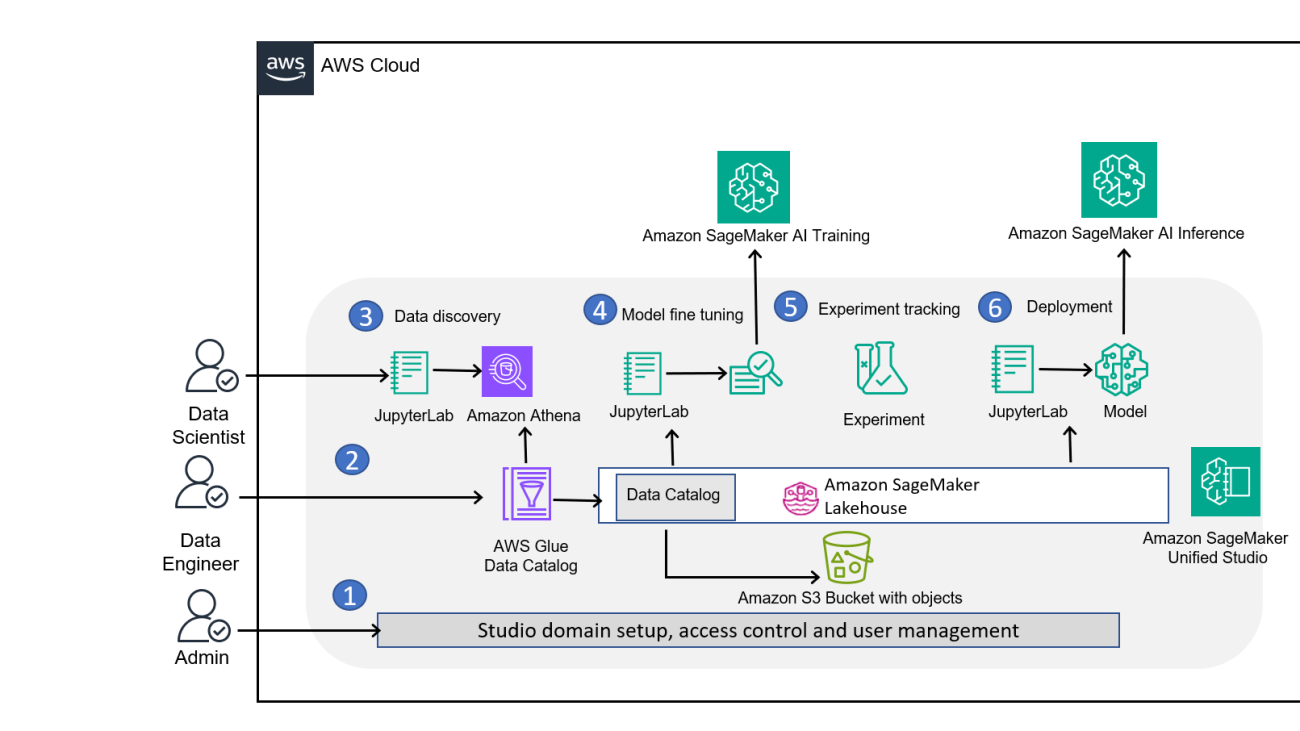
The following diagram illustrates the solution architecture. There are three personas: admin, data engineer, and user, which can be a data scientist or an ML engineer.

AWS SageMaker Unified Studio ML workflow showing data processing, model training, and deployment stages

Setting up the solution consists of the following steps:

1. The admin sets up the SageMaker Unified Studio domain for the user and sets the access controls. The admin also publishes the data to SageMaker Catalog in SageMaker Lakehouse.
2. Data engineers can create and manage extract, transform, and load (ETL) pipelines directly within Unified Studio using Visual ETL. They can transform raw data sources into datasets ready for exploratory data analysis. The admin can then manage the publication of these assets to the SageMaker Catalog, making them discoverable and accessible to other team members or users such as data engineers in the organization.
3. Users or data engineers can log in to the Unified Studio web-based IDE using the login provided by the admin to create a project and create a managed MLflow server for tracking experiments. Users can discover available data assets in the SageMaker Catalog and request a subscription to an asset published by the data engineer. After the data engineer approves the subscription request, the user performs an exploratory data analysis of the content of the table with the query editor or with a JupyterLab notebook, then prepares the dataset by connecting with SageMaker Catalog through an AWS Glue or Athena connection.
4. You can explore models from SageMaker JumpStart, which hosts over 200 models for various tasks, and fine-tune directly with the UI, or develop a training script for fine-tuning the LLM in the JupyterLab IDE. SageMaker AI provides distributed training libraries and supports various distributed training options for deep learning tasks. For this post, we use the PyTorch framework and use Hugging Face open source FMs for fine-tuning. We will show you how you can use parameter efficient fine-tuning (PEFT) with Low-Rank Adaptation (LoRa), where you freeze the model weights, train the model with modifying weight metrics, and then merge these LoRa adapters back to the base model after distributed training.
5. You can track and monitor fine-tuning metrics directly in SageMaker Unified Studio using MLflow, by analyzing metrics such as loss to make sure the model is correctly fine-tuned.
6. You can deploy the model to a SageMaker AI endpoint after the fine-tuning job is complete and test it directly from SageMaker Unified Studio.

Prerequisites

Before starting this tutorial, make sure you have the following:

• An AWS account with permissions to create SageMaker resources. For setup instructions, see Set up an AWS account and create an administrator user.
• Familiarity with Python and PyTorch for distributed training and model customization.

Set up SageMaker Unified Studio and configure user access

SageMaker Unified Studio is built on top of Amazon DataZone capabilities such as domains to organize your assets and users, and projects to collaborate with others users, securely share artifacts, and seamlessly work across compute services.

To set up Unified Studio, complete the following steps:

1. As an admin, create a SageMaker Unified Studio domain, and note the URL.
2. On the domain’s details page, on the User management tab, choose Configure SSO user access. For this post, we recommend setting up using single sign-on (SSO) access using the URL.

For more information about setting up user access, see Managing users in Amazon SageMaker Unified Studio.

Log in to SageMaker Unified Studio

Now that you have created your new SageMaker Unified Studio domain, complete the following steps to access SageMaker Unified Studio:

1. On the SageMaker console, open the details page of your domain.
2. Choose the link for the SageMaker Unified Studio URL.
3. Log in with your SSO credentials.

Now you’re signed in to SageMaker Unified Studio.

Create a project

The next step is to create a project. Complete the following steps:

1. In SageMaker Unified Studio, choose Select a project on the top menu, and choose Create project.
2. For Project name, enter a name (for example, demo).
3. For Project profile, choose your profile capabilities. A project profile is a collection of blueprints, which are configurations used to create projects. For this post, we choose All capabilities, then choose Continue.

Creating a project in Amazon SageMaker Unified Studio

Create a compute space

SageMaker Unified Studio provides compute spaces for IDEs that you can use to code and develop your resources. By default, it creates a space for you to get started with you project. You can find the default space by choosing Compute in the navigation pane and choosing the Spaces tab. You can then choose Open to go to the JuypterLab environment and add members to this space. You can also create a new space by choosing Create space on the Spaces tab.

To use SageMaker Studio notebooks cost-effectively, use smaller, general-purpose instances (like the T or M families) for interactive data exploration and prototyping. For heavy lifting like training or large-scale processing or deployment, use SageMaker AI training jobs and SageMaker AI prediction to offload the work to separate and more powerful instances such as the P5 family. We will show you in the notebook how you can run training jobs and deploy LLMs in the notebook with APIs. It is not recommended to run distributed workloads in notebook instances. The chances of kernel failures is high because JupyterLab notebooks should not be used for large distributed workloads (both for data and ML training).

The following screenshot shows the configuration options for your space. You can change your instance size from default (ml.t3.medium) to (ml.m5.xlarge) for the JupyterLab IDE. You can also increase the Amazon Elastic Block Store (Amazon EBS) volume capacity from 16 GB to 50 GB for training LLMs.

Canfigure space in Amazon SageMaker Unified Studio

Set up MLflow to track ML experiments

You can use MLflow in SageMaker Unified Studio to create, manage, analyze, and compare ML experiments. Complete the following steps to set up MLflow:

1. In SageMaker Unified Studio, choose Compute in the navigation pane.
2. On the MLflow Tracking Servers tab, choose Create MLflow Tracking Server.
3. Provide a name and create your tracking server.
4. Choose Copy ARN to copy the Amazon Resource Name (ARN) of the tracking server.

You will need this MLflow ARN in your notebook to set up distributed training experiment tracking.

Set up the data catalog

For model fine-tuning, you need access to a dataset. After you set up the environment, the next step is to find the relevant data from the SageMaker Unified Studio data catalog and prepare the data for model tuning. For this post, we use the Stanford Question Answering Dataset (SQuAD) dataset. This dataset is a reading comprehension dataset, consisting of questions posed by crowd workers on a set of Wikipedia articles, where the answer to every question is a segment of text, or span, from the corresponding reading passage, or the question might be unanswerable.

Download the SQuaD dataset and upload it to SageMaker Lakehouse by following the steps in Uploading data.

Adding data to Catalog in Amazon SageMaker Unified Studio

To make this data discoverable by the users or ML engineers, the admin needs to publish this data to the Data Catalog. For this post, you can directly download the SQuaD dataset and upload it to the catalog. To learn how to publish the dataset to SageMaker Catalog, see Publish assets to the Amazon SageMaker Unified Studio catalog from the project inventory.

Query data with the query editor and JupyterLab

In many organizations, data preparation is a collaborative effort. A data engineer might prepare an initial raw dataset, which a data scientist then refines and augments with feature engineering before using it for model training. In the SageMaker Lakehouse data and model catalog, publishers set subscriptions for automatic or manual approval (wait for admin approval). Because you already set up the data in the previous section, you can skip this section showing how to subscribe to the dataset.

To subscribe to another dataset like SQuAD, open the data and model catalog in Amazon SageMaker Lakehouse, choose SQuAD, and subscribe.

Subscribing to any asset or dataset published by Admin

Next, let’s use the data explorer to explore the dataset you subscribed to. Complete the following steps:

1. On the project page, choose Data.
2. Under Lakehouse, expand AwsDataCatalog.
3. Expand your database starting from glue_db_.
4. Choose the dataset you created (starting with squad) and choose Query with Athena.

Querying the data using Query Editor in Amazon SageMaker Unfied Studio

Process your data through a multi-compute JupyterLab IDE notebook

SageMaker Unified Studio provides a unified JupyterLab experience across different languages, including SQL, PySpark, Python, and Scala Spark. It also supports unified access across different compute runtimes such as Amazon Redshift and Athena for SQL, Amazon EMR Serverless, Amazon EMR on EC2, and AWS Glue for Spark.

Complete the following steps to get started with the unified JupyterLab experience:

1. Open your SageMaker Unified Studio project page.
2. On the top menu, choose Build, and under IDE & APPLICATIONS, choose JupyterLab.
3. Wait for the space to be ready.
4. Choose the plus sign and for Notebook, choose Python 3.
5. Open a new terminal and enter git clonehttps://github.com/aws-samples/amazon-sagemaker-generativeai.
6. Go to the folder amazon-sagemaker-generativeai/3_distributed_training/distributed_training_sm_unified_studio/ and open the distributed training in unified studio.ipynb notebook to get started.
7. Enter the MLflow server ARN you created in the following code:

import os
os.environ["mlflow_uri"] = ""
os.environ["mlflow_experiment_name"] = "deepseek-r1-distill-llama-8b-sft"

Now you an visualize the data through the notebook.

8. On the project page, choose Data.
9. Under Lakehouse, expand AwsDataCatalog.
10. Expand your database starting from glue_db, copy the name of the database, and enter it in the following code:

db_name = "<enter your db name>"
table = "sqad"

11. You can now access the entire dataset directly by using the in-line SQL query capabilities of JupyterLab notebooks in SageMaker Unified Studio. You can follow the data preprocessing steps in the notebook.

%%sql project.athena
SELECT * FROM "<DATABASE_NAME>"."sqad";

The following screenshot shows the output.

We are going to split the dataset into a test set and training set for model training. When the data processing in done and we have split the data into test and training sets, the next step is to perform fine-tuning of the model using SageMaker Distributed Training.

Fine-tune the model with SageMaker Distributed training

You’re now ready to fine-tune your model by using SageMaker AI capabilities for training. Amazon SageMaker Training is a fully managed ML service offered by SageMaker that helps you efficiently train a wide range of ML models at scale. The core of SageMaker AI jobs is the containerization of ML workloads and the capability of managing AWS compute resources. SageMaker Training takes care of the heavy lifting associated with setting up and managing infrastructure for ML training workloads

We select one model directly from the Hugging Face Hub, DeepSeek-R1-Distill-Llama-8B, and develop our training script in the JupyterLab space. Because we want to distribute the training across all the available GPUs in our instance, by using PyTorch Fully Sharded Data Parallel (FSDP), we use the Hugging Face Accelerate library to run the same PyTorch code across distributed configurations. You can start the fine-tuning job directly in your JupyterLab notebook or use the SageMaker Python SDK to start the training job. We use the Trainer from transfomers to fine-tune our model. We prepared the script train.py, which loads the dataset from disk, prepares the model and tokenizer, and starts the training.

For configuration, we use TrlParser, and provide hyperparameters in a YAML file. You can upload this file and provide it to SageMaker similar to your datasets. The following is the config file for fine-tuning the model on ml.g5.12xlarge. Save the config file as args.yaml and upload it to Amazon Simple Storage Service (Amazon S3).

cat > ./args.yaml <<EOF
model_id: "deepseek-ai/DeepSeek-R1-Distill-Llama-8B"       # Hugging Face model id
mlflow_uri: "${mlflow_uri}"
mlflow_experiment_name: "${mlflow_experiment_name}"
# sagemaker specific parameters
output_dir: "/opt/ml/model"                       # path to where SageMaker will upload the model 
train_dataset_path: "/opt/ml/input/data/train/"   # path to where FSx saves train dataset
test_dataset_path: "/opt/ml/input/data/test/"     # path to where FSx saves test dataset
# training parameters
lora_r: 8
lora_alpha: 16
lora_dropout: 0.1                 
learning_rate: 2e-4                    # learning rate scheduler
num_train_epochs: 1                    # number of training epochs
per_device_train_batch_size: 2         # batch size per device during training
per_device_eval_batch_size: 1          # batch size for evaluation
gradient_accumulation_steps: 2         # number of steps before performing a backward/update pass
gradient_checkpointing: true           # use gradient checkpointing
bf16: true                             # use bfloat16 precision
tf32: false                            # use tf32 precision
fsdp: "full_shard auto_wrap offload"
fsdp_config: 
    backward_prefetch: "backward_pre"
    cpu_ram_efficient_loading: true
    offload_params: true
    forward_prefetch: false
    use_orig_params: true
merge_weights: true                    # merge weights in the base model
EOF

Use the following code to use the native PyTorch container image, pre-built for SageMaker:

image_uri = sagemaker.image_uris.retrieve(
    framework="pytorch",
    region=sagemaker_session.boto_session.region_name,
    version="2.6.0",
    instance_type=instance_type,
    image_scope="training"
)

image_uri

Define the trainer as follows:

Define the ModelTrainer
model_trainer = ModelTrainer(
    training_image=image_uri,
    source_code=source_code,
    base_job_name=job_name,
    compute=compute_configs,
    distributed=Torchrun(),
    stopping_condition=StoppingCondition(
        max_runtime_in_seconds=7200
    ),
    hyperparameters={
        "config": "/opt/ml/input/data/config/args.yaml" # path to TRL config which was uploaded to s3
    },
    output_data_config=OutputDataConfig(
        s3_output_path=output_path
    ),
)

Run the trainer with the following:

# starting the train job with our uploaded datasets as input
model_trainer.train(input_data_config=data, wait=True)

You can follow the steps in the notebook.

You can explore the job execution in SageMaker Unified Studio. The training job runs on the SageMaker training cluster by distributing the computation across the four available GPUs on the selected instance type ml.g5.12xlarge. We choose to merge the LoRA adapter with the base model. This decision was made during the training process by setting the merge_weights parameter to True in our train_fn() function. Merging the weights provides a single, cohesive model that incorporates both the base knowledge and the domain-specific adaptations we’ve made through fine-tuning.

Track training metrics and model registration using MLflow

You created an MLflow server in an earlier step to track experiments and registered models, and provided the server ARN in the notebook.

You can log MLflow models and automatically register them with Amazon SageMaker Model Registry using either the Python SDK or directly through the MLflow UI. Use mlflow.register_model() to automatically register a model with SageMaker Model Registry during model training. You can explore the MLflow tracking code in train.py and the notebook. The training code tracks MLflow experiments and registers the model to the MLflow model registry. To learn more, see Automatically register SageMaker AI models with SageMaker Model Registry.

To see the logs, complete the following steps:

1. Choose Build, then choose Spaces.
2. Choose Compute in the navigation pane.
3. On the MLflow Tracking Servers tab, choose Open to open the tracking server.

You can see both the experiments and registered models.

Deploy and test the model using SageMaker AI Inference

When deploying a fine-tuned model on AWS, SageMaker AI Inference offers multiple deployment strategies. In this post, we use SageMaker real-time inference. The real-time inference endpoint is designed for having full control over the inference resources. You can use a set of available instances and deployment options for hosting your model. By using the SageMaker built-in container DJL Serving, you can take advantage of the inference script and optimization options available directly in the container. In this post, we deploy the fine-tuned model to a SageMaker endpoint for running inference, which will be used for testing the model.

In SageMaker Unified Studio, in JupyterLab, we create the Model object, which is a high-level SageMaker model class for working with multiple container options. The image_uri parameter specifies the container image URI for the model, and model_data points to the Amazon S3 location containing the model artifact (automatically uploaded by the SageMaker training job). We also specify a set of environment variables to configure the specific inference backend option (OPTION_ROLLING_BATCH), the degree of tensor parallelism based on the number of available GPUs (OPTION_TENSOR_PARALLEL_DEGREE), and the maximum allowable length of input sequences (in tokens) for models during inference (OPTION_MAX_MODEL_LEN).

model = Model(
    image_uri=image_uri,
    model_data=f"s3://{bucket_name}/{job_prefix}/{job_name}/output/model.tar.gz",
    role=get_execution_role(),
    env={
        'HF_MODEL_ID': "/opt/ml/model",
        'OPTION_TRUST_REMOTE_CODE': 'true',
        'OPTION_ROLLING_BATCH': "vllm",
        'OPTION_DTYPE': 'bf16',
        'OPTION_TENSOR_PARALLEL_DEGREE': 'max',
        'OPTION_MAX_ROLLING_BATCH_SIZE': '1',
        'OPTION_MODEL_LOADING_TIMEOUT': '3600',
        'OPTION_MAX_MODEL_LEN': '4096'
    }
)

After you create the model object, you can deploy it to an endpoint using the deploy method. The initial_instance_count and instance_type parameters specify the number and type of instances to use for the endpoint. We selected the ml.g5.4xlarge instance for the endpoint. The container_startup_health_check_timeout and model_data_download_timeout parameters set the timeout values for the container startup health check and model data download, respectively.

model_id = "deepseek-ai/DeepSeek-R1-Distill-Llama-8B"
endpoint_name = f"{model_id.split('/')[-1].replace('.', '-')}-sft-djl"
predictor = model.deploy(
    initial_instance_count=instance_count,
    instance_type=instance_type,
    container_startup_health_check_timeout=1800,
    model_data_download_timeout=3600
)

It takes a few minutes to deploy the model before it becomes available for inference and evaluation. You can test the endpoint invocation in JupyterLab, by using the AWS SDK with the boto3 client for sagemaker-runtime, or by using the SageMaker Python SDK and the predictor previously created, by using the predict API.

base_prompt = f"""<s> [INST] {{question}} [/INST] """

prompt = base_prompt.format(
    question="What statue is in front of the Notre Dame building?"
)

predictor.predict({
    "inputs": prompt,
    "parameters": {
        "max_new_tokens": 300,
        "temperature": 0.2,
        "top_p": 0.9,
        "return_full_text": False,
        "stop": ['</s>']
    }
})

You can also test the model invocation in SageMaker Unified Studio, on the Inference endpoint page and Text inference tab.

Troubleshooting

You might encounter some of the following errors while running your model training and deployment:

• Training job fails to start – If a training job fails to start, make sure your IAM role AmazonSageMakerDomainExecution has the necessary permissions, verify the instance type is available in your AWS Region, and check your S3 bucket permissions. This role is created when an admin creates the domain, and you can ask the admin to check your IAM access permissions associated with this role.
• Out-of-memory errors during training – If you encounter out-of-memory errors during training, try reducing the batch size, use gradient accumulation to simulate larger batches, or consider using a larger instance.
• Slow model deployment – For slow model deployment, make sure model artifacts aren’t excessively large, and use appropriate instance types for inference and capacity available for that instance in your Region.

For more troubleshooting tips, refer to Troubleshooting guide.

Clean up

SageMaker Unified Studio by default shuts down idle resources such as JupyterLab spaces after 1 hour. However, you must delete the S3 bucket and the hosted model endpoint to stop incurring costs. You can delete the real-time endpoints you created using the SageMaker console. For instructions, see Delete Endpoints and Resources.

Conclusion

This post demonstrated how SageMaker Unified Studio serves as a powerful centralized service for data and AI workflows, showcasing its seamless integration capabilities throughout the fine-tuning process. With SageMaker Unified Studio, data engineers and ML practitioners can efficiently discover and access data through SageMaker Catalog, prepare datasets, fine-tune models, and deploy them—all within a single, unified environment. The service’s direct integration with SageMaker AI and various AWS analytics services streamlines the development process, alleviating the need to switch between multiple tools and environments. The solution highlights the service’s versatility in handling complex ML workflows, from data discovery and preparation to model deployment, while maintaining a cohesive and intuitive user experience. Through features like integrated MLflow tracking, built-in model monitoring, and flexible deployment options, SageMaker Unified Studio demonstrates its capability to support sophisticated AI/ML projects at scale.

To learn more about SageMaker Unified Studio, see An integrated experience for all your data and AI with Amazon SageMaker Unified Studio.

If this post helps you or inspires you to solve a problem, we would love to hear about it! The code for this solution is available on the GitHub repo for you to use and extend. Contributions are always welcome!

About the authors

Mona Mona currently works as a Sr World Wide Gen AI Specialist Solutions Architect at Amazon focusing on Gen AI Solutions. She was a Lead Generative AI specialist in Google Public Sector at Google before joining Amazon. She is a published author of two books – Natural Language Processing with AWS AI Services and Google Cloud Certified Professional Machine Learning Study Guide. She has authored 19 blogs on AI/ML and cloud technology and a co-author on a research paper on CORD19 Neural Search which won an award for Best Research Paper at the prestigious AAAI (Association for the Advancement of Artificial Intelligence) conference.

Bruno Pistone is a Senior Generative AI and ML Specialist Solutions Architect for AWS based in Milan. He works with large customers helping them to deeply understand their technical needs and design AI and Machine Learning solutions that make the best use of the AWS Cloud and the Amazon Machine Learning stack. His expertise include: Machine Learning end to end, Machine Learning Industrialization, and Generative AI. He enjoys spending time with his friends and exploring new places, as well as travelling to new destinations.

Lauren Mullennex is a Senior GenAI/ML Specialist Solutions Architect at AWS. She has a decade of experience in DevOps, infrastructure, and ML. Her areas of focus include MLOps/LLMOps, generative AI, and computer vision.

Read More

Generative AI has revolutionized customer interactions across industries by offering personalized, intuitive experiences powered by unprecedented access to information. This transformation is further enhanced by Retrieval Augmented Generation (RAG), a technique that allows large language models (LLMs) to reference external knowledge sources beyond their training data. RAG has gained popularity for its ability to improve generative AI applications by incorporating additional information, often preferred by customers over techniques like fine-tuning due to its cost-effectiveness and faster iteration cycles.

The RAG approach excels in grounding language generation with external knowledge, producing more factual, coherent, and relevant responses. This capability proves invaluable in applications such as question answering, dialogue systems, and content generation, where accuracy and informative outputs are crucial. For businesses, RAG offers a powerful way to use internal knowledge by connecting company documentation to a generative AI model. When an employee asks a question, the RAG system retrieves relevant information from the company’s internal documents and uses this context to generate an accurate, company-specific response. This approach enhances the understanding and usage of internal company documents and reports. By extracting relevant context from corporate knowledge bases, RAG models facilitate tasks like summarization, information extraction, and complex question answering on domain-specific materials, enabling employees to quickly access vital insights from vast internal resources. This integration of AI with proprietary information can significantly improve efficiency, decision-making, and knowledge sharing across the organization.

A typical RAG workflow consists of four key components: input prompt, document retrieval, contextual generation, and output. The process begins with a user query, which is used to search a comprehensive knowledge corpus. Relevant documents are then retrieved and combined with the original query to provide additional context for the LLM. This enriched input allows the model to generate more accurate and contextually appropriate responses. RAG’s popularity stems from its ability to use frequently updated external data, providing dynamic outputs without the need for costly and compute-intensive model retraining.

To implement RAG effectively, many organizations turn to platforms like Amazon SageMaker JumpStart. This service offers numerous advantages for building and deploying generative AI applications, including access to a wide range of pre-trained models with ready-to-use artifacts, a user-friendly interface, and seamless scalability within the AWS ecosystem. By using pre-trained models and optimized hardware, SageMaker JumpStart enables rapid deployment of both LLMs and embedding models, minimizing the time spent on complex scalability configurations.

In the previous post, we showed how to build a RAG application on SageMaker JumpStart using Facebook AI Similarity Search (Faiss). In this post, we show how to use Amazon OpenSearch Service as a vector store to build an efficient RAG application.

Solution overview

To implement our RAG workflow on SageMaker, we use a popular open source Python library known as LangChain. With LangChain, the RAG components are simplified into independent blocks that you can bring together using a chain object that will encapsulate the entire workflow. The solution consists of the following key components:

• LLM (inference) – We need an LLM that will do the actual inference and answer the end-user’s initial prompt. For our use case, we use Meta Llama3 for this component. LangChain comes with a default wrapper class for SageMaker endpoints with which we can simply pass in the endpoint name to define an LLM object in the library.
• Embeddings model – We need an embeddings model to convert our document corpus into textual embeddings. This is necessary for when we’re doing a similarity search on the input text to see what documents share similarities or contain the information to help augment our response. For this post, we use the BGE Hugging Face Embeddings model available in SageMaker JumpStart.
• Vector store and retriever – To house the different embeddings we have generated, we use a vector store. In this case, we use OpenSearch Service, which allows for similarity search using k-nearest neighbors (k-NN) as well as traditional lexical search. Within our chain object, we define the vector store as the retriever. You can tune this depending on how many documents you want to retrieve.

The following diagram illustrates the solution architecture.

In the following sections, we walk through setting up OpenSearch, followed by exploring the notebook that implements a RAG solution with LangChain, Amazon SageMaker AI, and OpenSearch Service.

Benefits of using OpenSearch Service as a vector store for RAG

In this post, we showcase how you can use a vector store such as OpenSearch Service as a knowledge base and embedding store. OpenSearch Service offers several advantages when used for RAG in conjunction with SageMaker AI:

• Performance – Efficiently handles large-scale data and search operations
• Advanced search – Offers full-text search, relevance scoring, and semantic capabilities
• AWS integration – Seamlessly integrates with SageMaker AI and other AWS services
• Real-time updates – Supports continuous knowledge base updates with minimal delay
• Customization – Allows fine-tuning of search relevance for optimal context retrieval
• Reliability – Provides high availability and fault tolerance through a distributed architecture
• Analytics – Provides analytical features for data understanding and performance improvement
• Security – Offers robust features such as encryption, access control, and audit logging
• Cost-effectiveness – Serves as an economical solution compared to proprietary vector databases
• Flexibility – Supports various data types and search algorithms, offering versatile storage and retrieval options for RAG applications

You can use SageMaker AI with OpenSearch Service to create powerful and efficient RAG systems. SageMaker AI provides the machine learning (ML) infrastructure for training and deploying your language models, and OpenSearch Service serves as an efficient and scalable knowledge base for retrieval.

OpenSearch Service optimization strategies for RAG

Based on our learnings from the hundreds of RAG applications deployed using OpenSearch Service as a vector store, we’ve developed several best practices:

• If you are starting from a clean slate and want to move quickly with something simple, scalable, and high-performing, we recommend using an Amazon OpenSearch Serverless vector store collection. With OpenSearch Serverless, you benefit from automatic scaling of resources, decoupling of storage, indexing compute, and search compute, with no node or shard management, and you only pay for what you use.
• If you have a large-scale production workload and want to take the time to tune for the best price-performance and the most flexibility, you can use an OpenSearch Service managed cluster. In a managed cluster, you pick the node type, node size, number of nodes, and number of shards and replicas, and you have more control over when to scale your resources. For more details on best practices for operating an OpenSearch Service managed cluster, see Operational best practices for Amazon OpenSearch Service.
• OpenSearch supports both exact k-NN and approximate k-NN. Use exact k-NN if the number of documents or vectors in your corpus is less than 50,000 for the best recall. For use cases where the number of vectors is greater than 50,000, exact k-NN will still provide the best recall but might not provide sub-100 millisecond query performance. Use approximate k-NN in use cases above 50,000 vectors for the best performance.
• OpenSearch uses algorithms from the NMSLIB, Faiss, and Lucene libraries to power approximate k-NN search. There are pros and cons to each k-NN engine, but we find that most customers choose Faiss due to its overall performance in both indexing and search as well as the variety of different quantization and algorithm options that are supported and the broad community support.
• Within the Faiss engine, OpenSearch supports both Hierarchical Navigable Small World (HNSW) and Inverted File System (IVF) algorithms. Most customers find HNSW to have better recall than IVF and choose it for their RAG use cases. To learn more about the differences between these engine algorithms, see Vector search.
• To reduce the memory footprint to lower the cost of the vector store while keeping the recall high, you can start with Faiss HNSW 16-bit scalar quantization. This can also reduce search latencies and improve indexing throughput when used with SIMD optimization.
• If using an OpenSearch Service managed cluster, refer to Performance tuning for additional recommendations.

Prerequisites

Make sure you have access to one ml.g5.4xlarge and ml.g5.2xlarge instance each in your account. A secret should be created in the same region as the stack is deployed.Then complete the following prerequisite steps to create a secret using AWS Secrets Manager:

1. On the Secrets Manager console, choose Secrets in the navigation pane.
2. Choose Store a new secret.

3. For Secret type, select Other type of secret.
4. For Key/value pairs, on the Plaintext tab, enter a complete password.
5. Choose Next.

6. For Secret name, enter a name for your secret.
7. Choose Next.

8. Under Configure rotation, keep the settings as default and choose Next.

9. Choose Store to save your secret.

10. On the secret details page, note the secret Amazon Resource Name (ARN) to use in the next step.

Create an OpenSearch Service cluster and SageMaker notebook

We use AWS CloudFormation to deploy our OpenSearch Service cluster, SageMaker notebook, and other resources. Complete the following steps:

1. Launch the following CloudFormation template.
2. Provide the ARN of the secret you created as a prerequisite and keep the other parameters as default.

3. Choose Create to create your stack, and wait for the stack to complete (about 20 minutes).
4. When the status of the stack is CREATE_COMPLETE, note the value of OpenSearchDomainEndpoint on the stack Outputs tab.
5. Locate SageMakerNotebookURL in the outputs and choose the link to open the SageMaker notebook.

Run the SageMaker notebook

After you have launched the notebook in JupyterLab, complete the following steps:

1. Go to genai-recipes/RAG-recipes/llama3-RAG-Opensearch-langchain-SMJS.ipynb.

You can also clone the notebook from the GitHub repo.

1. Update the value of OPENSEARCH_URL in the notebook with the value copied from OpenSearchDomainEndpoint in the previous step (look for os.environ['OPENSEARCH_URL'] = "").  The port needs to be 443.
2. Run the cells in the notebook.

The notebook provides a detailed explanation of all the steps. We explain some of the key cells in the notebook in this section.

For the RAG workflow, we deploy the huggingface-sentencesimilarity-bge-large-en-v1-5 embedding model and meta-textgeneration-llama-3-8b-instruct LLM from Hugging Face. SageMaker JumpStart simplifies this process because the model artifacts, data, and container specifications are all prepackaged for optimal inference. These are then exposed using the SageMaker Python SDK high-level API calls, which let you specify the model ID for deployment to a SageMaker real-time endpoint:

 sagemaker.jumpstart.model  JumpStartModel

model_id  "meta-textgeneration-llama-3-8b-instruct"
accept_eula  
model  JumpStartModel(model_idmodel_id)
llm_predictor  modeldeploy(accept_eulaaccept_eula)

model_id  "huggingface-sentencesimilarity-bge-large-en-v1-5"
text_embedding_model  JumpStartModel(model_idmodel_id)
embedding_predictor  text_embedding_modeldeploy()

Content handlers are crucial for formatting data for SageMaker endpoints. They transform inputs into the format expected by the model and handle model-specific parameters like temperature and token limits. These parameters can be tuned to control the creativity and consistency of the model’s responses.

class Llama38BContentHandler(LLMContentHandler):
    content_type = "application/json"
    accepts = "application/json"

    def transform_input(self, prompt: str, model_kwargs: dict) -> bytes:
        payload = {
            "inputs": prompt,
            "parameters": {
                "max_new_tokens": 1000,
                "top_p": 0.9,
                "temperature": 0.6,
                "stop": ["<|eot_id|>"],
            },
        }
        input_str = json.dumps(
            payload,
        )
        #print(input_str)
        return input_str.encode("utf-8")

We use PyPDFLoader from LangChain to load PDF files, attach metadata to each document fragment, and then use RecursiveCharacterTextSplitter to break the documents into smaller, manageable chunks. The text splitter is configured with a chunk size of 1,000 characters and an overlap of 100 characters, which helps maintain context between chunks. This preprocessing step is crucial for effective document retrieval and embedding generation, because it makes sure the text segments are appropriately sized for the embedding model and the language model used in the RAG system.

import numpy as np
from langchain_community.document_loaders import PyPDFLoader
from langchain.text_splitter import RecursiveCharacterTextSplitter
documents = []
for idx, file in enumerate(filenames):
    loader = PyPDFLoader(data_root + file)
    document = loader.load()
    for document_fragment in document:
        document_fragment.metadata = metadata[idx]
    documents += document
# - in our testing Character split works better with this PDF data set
text_splitter = RecursiveCharacterTextSplitter(
    # Set a really small chunk size, just to show.
    chunk_size=1000,
    chunk_overlap=100,
)
docs = text_splitter.split_documents(documents)
print(docs[100])

The following block initializes a vector store using OpenSearch Service for the RAG system. It converts preprocessed document chunks into vector embeddings using a SageMaker model and stores them in OpenSearch Service. The process is configured with security measures like SSL and authentication to provide secure data handling. The bulk insertion is optimized for performance with a sizeable batch size. Finally, the vector store is wrapped with VectorStoreIndexWrapper, providing a simplified interface for operations like querying and retrieval. This setup creates a searchable database of document embeddings, enabling quick and relevant context retrieval for user queries in the RAG pipeline.

from langchain.indexes.vectorstore import VectorStoreIndexWrapper
# Initialize OpenSearchVectorSearch
vectorstore_opensearch = OpenSearchVectorSearch.from_documents(
    docs,
    sagemaker_embeddings,
    http_auth=awsauth,  # Auth will use the IAM role
    use_ssl=True,
    verify_certs=True,
    connection_class=RequestsHttpConnection,
    bulk_size=2000  # Increase this to accommodate the number of documents you have
)
# Wrap the OpenSearch vector store with the VectorStoreIndexWrapper
wrapper_store_opensearch = VectorStoreIndexWrapper(vectorstore=vectorstore_opensearch)

Next, we use the wrapper from the previous step along with the prompt template. We define the prompt template for interacting with the Meta Llama 3 8B Instruct model in the RAG system. The template uses specific tokens to structure the input in a way that the model expects. It sets up a conversation format with system instructions, user query, and a placeholder for the assistant’s response. The PromptTemplate class from LangChain is used to create a reusable prompt with a variable for the user’s query. This structured approach to prompt engineering helps maintain consistency in the model’s responses and guides it to act as a helpful assistant.

prompt_template = """<|begin_of_text|><|start_header_id|>system<|end_header_id|>
You are a helpful assistant.
<|eot_id|><|start_header_id|>user<|end_header_id|>
{query}
<|eot_id|><|start_header_id|>assistant<|end_header_id|>
"""
PROMPT = PromptTemplate(
    template=prompt_template, input_variables=["query"]
)
query = "How did AWS perform in 2021?"

answer = wrapper_store_opensearch.query(question=PROMPT.format(query=query), llm=llm)
print(answer)

Similarly, the notebook also shows how to use Retrieval QA, where you can customize how the documents fetched should be added to prompt using the chain_type parameter.

Clean up

Delete your SageMaker endpoints from the notebook to avoid incurring costs:

# Delete resources
llm_predictor.delete_model()
llm_predictor.delete_endpoint()
embedding_predictor.delete_model()
embedding_predictor.delete_endpoint()

Next, delete your OpenSearch cluster to stop incurring additional charges:aws cloudformation delete-stack --stack-name rag-opensearch

Conclusion

RAG has revolutionized how businesses use AI by enabling general-purpose language models to work seamlessly with company-specific data. The key benefit is the ability to create AI systems that combine broad knowledge with up-to-date, proprietary information without expensive model retraining. This approach transforms customer engagement and internal operations by delivering personalized, accurate, and timely responses based on the latest company data. The RAG workflow—comprising input prompt, document retrieval, contextual generation, and output—allows businesses to tap into their vast repositories of internal documents, policies, and data, making this information readily accessible and actionable. For businesses, this means enhanced decision-making, improved customer service, and increased operational efficiency. Employees can quickly access relevant information, while customers receive more accurate and personalized responses. Moreover, RAG’s cost-efficiency and ability to rapidly iterate make it an attractive solution for businesses looking to stay competitive in the AI era without constant, expensive updates to their AI systems. By making general-purpose LLMs work effectively on proprietary data, RAG empowers businesses to create dynamic, knowledge-rich AI applications that evolve with their data, potentially transforming how companies operate, innovate, and engage with both employees and customers.

SageMaker JumpStart has streamlined the process of developing and deploying generative AI applications. It offers pre-trained models, user-friendly interfaces, and seamless scalability within the AWS ecosystem, making it straightforward for businesses to harness the power of RAG.

Furthermore, using OpenSearch Service as a vector store facilitates swift retrieval from vast information repositories. This approach not only enhances the speed and relevance of responses, but also helps manage costs and operational complexity effectively.

By combining these technologies, you can create robust, scalable, and efficient RAG systems that provide up-to-date, context-aware responses to customer queries, ultimately enhancing user experience and satisfaction.

To get started with implementing this Retrieval Augmented Generation (RAG) solution using Amazon SageMaker JumpStart and Amazon OpenSearch Service, check out the example notebook on GitHub. You can also learn more about Amazon OpenSearch Service in the developer guide.

About the authors

Vivek Gangasani is a Lead Specialist Solutions Architect for Inference at AWS. He helps emerging generative AI companies build innovative solutions using AWS services and accelerated compute. Currently, he is focused on developing strategies for fine-tuning and optimizing the inference performance of large language models. In his free time, Vivek enjoys hiking, watching movies, and trying different cuisines.

Harish Rao is a Senior Solutions Architect at AWS, specializing in large-scale distributed AI training and inference. He empowers customers to harness the power of AI to drive innovation and solve complex challenges. Outside of work, Harish embraces an active lifestyle, enjoying the tranquility of hiking, the intensity of racquetball, and the mental clarity of mindfulness practices.

Raghu Ramesha is an ML Solutions Architect. He specializes in machine learning, AI, and computer vision domains, and holds a master’s degree in Computer Science from UT Dallas. In his free time, he enjoys traveling and photography.

Sohaib Katariwala is a Sr. Specialist Solutions Architect at AWS focused on Amazon OpenSearch Service. His interests are in all things data and analytics. More specifically he loves to help customers use AI in their data strategy to solve modern day challenges.

Karan Jain is a Senior Machine Learning Specialist at AWS, where he leads the worldwide Go-To-Market strategy for Amazon SageMaker Inference. He helps customers accelerate their generative AI and ML journey on AWS by providing guidance on deployment, cost-optimization, and GTM strategy. He has led product, marketing, and business development efforts across industries for over 10 years, and is passionate about mapping complex service features to customer solutions.

Read More

Just as APIs became the standard for integration, AI agents are transforming workflow automation through intelligent task coordination. AI agents are already enhancing decision-making and streamlining operations across enterprises. But as adoption accelerates, organizations face growing complexity in managing them at scale. Organizations struggle with observability and lifecycle management, finding it difficult to monitor performance and manage versions effectively. Governance and security concerns arise as these agents process sensitive data, which requires strict compliance and access controls. Perhaps most concerningly, without proper management, organizations face the risk of agent sprawl—the unchecked proliferation of AI agents leading to inefficiency and security vulnerabilities.

Boomi and AWS have collaborated to address the complexity surrounding AI agents with Agent Control Tower, an AI agent management solution developed by Boomi and tightly integrated with Amazon Bedrock. Agent Control Tower, part of the Boomi Agentstudio solution, provides the governance framework to manage this transformation, with capabilities that address both current and emerging compliance needs.

As a leader in enterprise iPaaS per Gartner’s Magic Quadrant, based on Completeness of Vision and Ability to Execute, Boomi serves over 20,000 enterprise customers, with three-quarters of these customers operating on AWS. This includes a significant presence among Fortune 500 and Global 2000 organizations across critical sectors such as healthcare, finance, technology, and manufacturing. Boomi is innovating with generative AI, with more than 2,000 customers using its AI agents. The convergence of capabilities that Boomi provides—spanning AI, integration, automation, API management, and data management—with AWS and its proven track record in reliability, security, and AI innovation creates a compelling foundation for standardized AI agent governance at scale. In this post, we share how Boomi partnered with AWS to help enterprises accelerate and scale AI adoption with confidence using Agent Control Tower.

A unified AI management solution

Built on AWS, Agent Control Tower uniquely delivers a single control plane for managing AI agents across multiple systems, including other cloud providers and on-premises environments. At its core, it offers comprehensive observability and monitoring, providing real-time performance tracking and deep visibility into agent decision-making and behavior.

The following screenshot showcases how users can view summary data across agent providers and add or manage providers.

The following screenshot shows an example of the Monitoring and Compliance dashboard.

Agent Control Tower also provides a single pane of glass for visibility into the tools used by each agent, as illustrated in the following screenshot.

Agent Control Tower provides key governance and security controls such as centralized policy enforcement and role-based access control, and enables meeting regulatory compliance with frameworks like GDPR and HIPAA. Furthermore, its lifecycle management capabilities enable automated agent discovery, version tracking, and operational control through features such as pause and resume functionality. Agent Control Tower is positioned as one of the first, if not the first, unified solutions that provides full lifecycle AI agent management with integrated governance and orchestration features. Although many vendors focus on releasing AI agents, there are few that focus on solutions for managing, deploying, and governing AI agents at scale.

The following screenshot shows an example of how users can review agent details and disable or enable an agent.

As shown in the following screenshot, users can drill down into details for each part of the agent.

Amazon Bedrock: Enabling and enhancing AI governance

Using Amazon Bedrock, organizations can implement security guardrails and content moderation while maintaining the flexibility to select and switch between AI models for optimized performance and accuracy. Organizations can create and enable access to curated knowledge bases and predefined action groups, enabling sophisticated multi-agent collaboration. Amazon Bedrock also provides comprehensive metrics and trace logs for agents to help facilitate complete transparency and accountability in agent operations. Through deep integration with Amazon Bedrock, Boomi’s Agent Control Tower enhances agent transparency and governance, offering a unified, actionable view of agent configurations and activities across environments.

The following diagram illustrates the Agent Control Tower architecture on AWS.

Business impact: Transforming enterprise AI operations

Consider a global manufacturer using AI agents for supply chain optimization. With Agent Control Tower, they can monitor agent performance across regions in real time, enforce consistent security policies, and enable regulatory compliance. When issues arise, they can quickly identify and resolve them while maintaining the ability to scale AI operations confidently. With this level of control and visibility, organizations can deploy AI agents more effectively while maintaining robust security and compliance standards.

Conclusion

Boomi customers have already deployed more than 33,000 agents and are seeing up to 80% less time spent on documentation and 50% faster issue resolution. With Boomi and AWS, enterprises can accelerate and scale AI adoption with confidence, backed by a product that puts visibility, governance, and security first. Discover how Agent Control Tower can help your organization manage AI agent sprawl and take advantage of scalable, compliance-aligned innovation. Take a guided tour and learn more about Boomi Agent Control Tower and Amazon Bedrock integration. Or, you can get started today with AI FastTrack.

About the authors

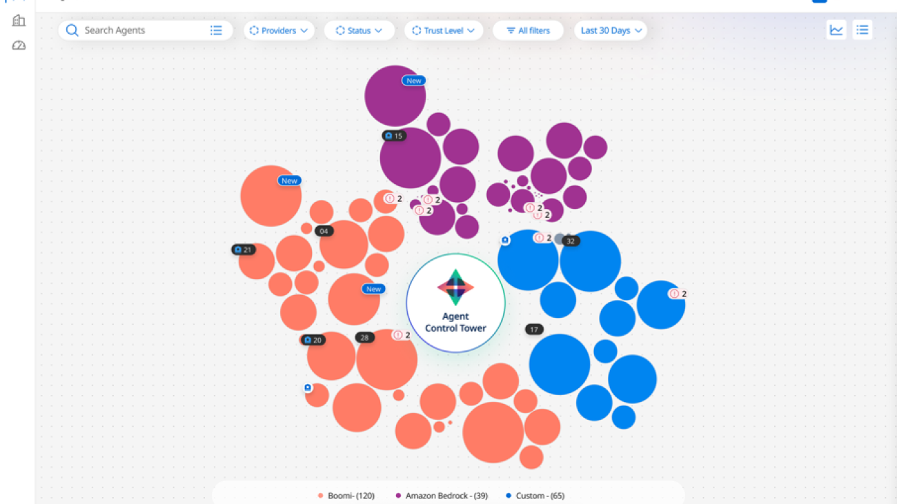
Deepak Chandrasekar is the VP of Software Engineering & User Experience and leads multidisciplinary teams at Boomi. He oversees flagship initiatives like Boomi’s Agent Control Tower, Task Automation, and Market Reach, while driving a cohesive and intelligent experience layer across products. Previously, Deepak held a key leadership role at Unifi Software, which was acquired by Boomi. With a passion for building scalable, and intuitive AI-powered solutions, he brings a commitment to engineering excellence and responsible innovation.

Sandeep Singh is Director of Engineering at Boomi, where he leads global teams building solutions that enable enterprise integration and automation at scale. He drives initiatives like Boomi Agent Control Tower, Marketplace, and Labs, empowering partners and customers with intelligent, trusted solutions. With leadership experience at GE and Fujitsu, Sandeep brings expertise in API strategy, product engineering, and AI/ML solutions. A former solution architect, he is passionate about designing mission-critical systems and driving innovation through scalable, intelligent solutions.

Santosh Ameti is a seasoned Engineering leader in the Amazon Bedrock team and has built Agents, Evaluation, Guardrails, and Prompt Management solutions. His team continuously innovates in the agentic space, delivering one of the most secure and managed agentic solutions for enterprises.

Greg Sligh is a Senior Solutions Architect at AWS with more than 25 years of experience in software engineering, software architecture, consulting, and IT and Engineering leadership roles across multiple industries. For the majority of his career, he has focused on creating and delivering distributed, data-driven applications with particular focus on scale, performance, and resiliency. Now he helps ISVs meet their objectives across technologies, with particular focus on AI/ML.

Padma Iyer is a Senior Customer Solutions Manager at Amazon Web Services, where she specializes in supporting ISVs. With a passion for cloud transformation and financial technology, Padma works closely with ISVs to guide them through successful cloud transformations, using best practices to optimize their operations and drive business growth. Padma has over 20 years of industry experience spanning banking, tech, and consulting.

Read More

Organizations face the challenge to manage data, multiple artificial intelligence and machine learning (AI/ML) tools, and workflows across different environments, impacting productivity and governance. A unified development environment consolidates data processing, model development, and AI application deployment into a single system. This integration streamlines workflows, enhances collaboration, and accelerates AI solution development from concept to production.

The next generation of Amazon SageMaker is the center for your data, analytics, and AI. SageMaker brings together AWS AI/ML and analytics capabilities and delivers an integrated experience for analytics and AI with unified access to data. Amazon SageMaker Unified Studio is a single data and AI development environment where you can find and access your data and act on it using AWS analytics and AI/ML services, for SQL analytics, data processing, model development, and generative AI application development.

With SageMaker Unified Studio, you can efficiently build generative AI applications in a trusted and secure environment using Amazon Bedrock. You can choose from a selection of high-performing foundation models (FMs) and advanced customization and tooling such as Amazon Bedrock Knowledge Bases, Amazon Bedrock Guardrails, Amazon Bedrock Agents, and Amazon Bedrock Flows. You can rapidly tailor and deploy generative AI applications, and share with the built-in catalog for discovery.

In this post, we demonstrate how you can use SageMaker Unified Studio to create complex AI workflows using Amazon Bedrock Flows.

Solution overview

Consider FinAssist Corp, a leading financial institution developing a generative AI-powered agent support application. The solution offers the following key features:

• Complaint reference system – An AI-powered system providing quick access to historical complaint data, enabling customer service representatives to efficiently handle customer follow-ups, support internal audits, and aid in training new staff.
• Intelligent knowledge base – A comprehensive data source of resolved complaints that quickly retrieves relevant complaint details, resolution actions, and outcome summaries.
• Streamlined workflow management – Enhanced consistency in customer communications through standardized access to past case information, supporting compliance checks and process improvement initiatives.
• Flexible query capability – A straightforward interface supporting various query scenarios, from customer inquiries about past resolutions to internal reviews of complaint handling procedures.

Let’s explore how SageMaker Unified Studio and Amazon Bedrock Flows, integrated with Amazon Bedrock Knowledge Bases and Amazon Bedrock Agents, address these challenges by creating an AI-powered complaint reference system. The following diagram illustrates the solution architecture.

The solution uses the following key components:

• SageMaker Unified Studio – Provides the development environment
• Flow app – Orchestrates the workflow, including:
  • Knowledge base queries
  • Prompt-based classification
  • Conditional routing
  • Agent-based response generation

The workflow processes user queries through the following steps:

1. A user submits a complaint-related question.
2. The knowledge base provides relevant complaint information.
3. The prompt classifies if the query is about resolution timing.
4. Based on the classification using the condition, the application takes the following action:
   1. Routes the query to an AI agent for specific resolution responses.
   2. Returns general complaint information.
5. The application generates an appropriate response for the user.

Prerequisites

For this example, you need the following:

• Access to SageMaker Unified Studio. (You will need the SageMaker Unified Studio portal URL from your administrator). You can authenticate using either:
  • AWS Identity and Access Management (IAM) user credentials.
  • Single sign-on (SSO) credentials with AWS IAM Identity Center.
• The IAM user or IAM Identity Center user must have appropriate permissions for:
  • SageMaker Unified Studio.
  • Amazon Bedrock (including Amazon Bedrock Flows, Amazon Bedrock Agents, Amazon Bedrock Prompt Management, and Amazon Bedrock Knowledge Bases).
  • For more information, refer to Identity-based policy examples.
• Access to Amazon Bedrock FMs (make sure these are enabled for your account), for example:Anthropic’s Claude 3 Haiku (for the agent).
• Configure access to your Amazon Bedrock serverless models for Amazon Bedrock in SageMaker Unified Studio projects.
• Amazon Titan Embedding (for the knowledge base).
• Sample complaint data prepared in CSV format for creating the knowledge base.

Prepare your data

We have created a sample dataset to use for Amazon Bedrock Knowledge Bases. This dataset has information of complaints received by customer service representatives and resolution information.The following is an example from the sample dataset:

complaint_id,product,sub_product,issue,sub_issue,complaint_summary,action_taken,next_steps,financial_institution,state,submitted_via,resolution_type,timely_response
FIN-2024-001,04/26/24,"Mortgage","Conventional mortgage","Payment issue","Escrow dispute","Customer disputes mortgage payment increase after recent escrow analysis","Reviewed escrow analysis, explained property tax increase impact, provided detailed payment breakdown","1. Send written explanation of escrow analysis 2. Schedule annual escrow review 3. Provide payment assistance options","Financial Institution-1","TX","Web","Closed with explanation","Yes"
FIN-2024-002,04/26/24,"Money transfer","Wire transfer","Processing delay","International transfer","Wire transfer of $10,000 delayed, customer concerned about international payment deadline","Located wire transfer in system, expedited processing, waived wire fee","1. Confirm receipt with receiving bank 2. Update customer on delivery 3. Document process improvement needs","Financial Institution-2","FL","Phone","Closed with monetary relief","No"

Create a project

In SageMaker Unified Studio, users can use projects to collaborate on various business use cases. Within projects, you can manage data assets in the SageMaker Unified Studio catalog, perform data analysis, organize workflows, develop ML models, build generative AI applications, and more.

To create a project, complete the following steps:

1. Open the SageMaker Unified Studio landing page using the URL from your admin.
2. Choose Create project.
3. Enter a project name and optional description.
4. For Project profile, choose Generative AI application development.
5. Choose Continue.

6. Complete your project configuration, then choose Create project.

Create a prompt

Let’s create a reusable prompt to capture the instructions for FMs, which we will use later while creating the flow application. For more information, see Reuse and share Amazon Bedrock prompts.

1. In SageMaker Unified Studio, on the Build menu, choose Prompt under Machine Learning & Generative AI.

2. Provide a name for the prompt.
3. Choose the appropriate FM (for this example, we choose Claude 3 Haiku).
4. For Prompt message, we enter the following:

You are a complaint analysis classifier. You will receive complaint data from a knowledge base. Analyze the {{input}} and respond with a single letter:
T: If the input contains information about complaint resolution timing, response time, or processing timeline (whether timely or delayed)
F: For all other types of complaint information
Return only 'T' or 'F' based on whether the knowledge base response is about resolution timing. Do not add any additional text or explanation - respond with just the single letter 'T' or 'F'.

5. Choose Save.

6. Choose Create version.

Create a chat agent

Let’s create a chat agent to handle specific resolution responses. Complete the following steps:

1. In SageMaker Unified Studio, on the Build menu, choose Chat agent under Machine Learning & Generative AI.
2. Provide a name for the prompt.
3. Choose the appropriate FM (for this example, we choose Claude 3 Haiku).
4. For Enter a system prompt, we enter the following:

You are a Financial Complaints Assistant AI. You will receive complaint information from a knowledge base and questions about resolution timing.
When responding to resolution timing queries:
1. Use the provided complaint information to confirm if it was resolved within timeline
2. For timely resolutions, provide:
   - Confirmation of timely completion
   - Specific actions taken (from the provided complaint data)
   - Next steps that were completed
2. For delayed resolutions, provide:
   - Acknowledgment of delay
   - Standard compensation package:
     • $75 service credit
     • Priority Status upgrade for 6 months
     • Service fees waived for current billing cycle
   - Actions taken (from the provided complaint data)
   - Contact information for follow-up: Priority Line: ************** 
Always reference the specific complaint details provided in your input when discussing actions taken and resolution process.

5. Choose Save.

6. After the agent is saved, choose Deploy.
7. For Alias name, enter demoAlias.
8. Choose Deploy.

Create a flow

Now that we have our prompt and agent ready, let’s create a flow that will orchestrate the complaint handling process:

1. In SageMaker Unified Studio, on the Build menu, choose Flow under Machine Learning & Generative AI.

2. Create a new flow called demo-flow.

Add a knowledge base to your flow application

Complete the following steps to add a knowledge base node to the flow:

1. In the navigation pane, on the Nodes tab, choose Knowledge Base.
2. On the Configure tab, provide the following information:
   1. For Node name, enter a name (for example, complaints_kb).
   2. Choose Create new Knowledge Base.
3. In the Create Knowledge Base pane, enter the following information:
   1. For Name, enter a name (for example, complaints).
   2. For Description, enter a description (for example, user complaints information).
   3. For Add data sources, select Local file and upload the complaints.txt file.
   4. For Embeddings model, choose Titan Text Embeddings V2.
   5. For Vector store, choose OpenSearch Serverless.
   6. Choose Create.

4. After you create the knowledge base, choose it in the flow.
5. In the details name, provide the following information:
6. For Response generation model, choose Claude 3 Haiku.
7. Connect the output of the flow input node with the input of the knowledge base node.
8. Connect the output of the knowledge base node with the input of the flow output node.

9. Choose Save.

Add a prompt to your flow application

Now let’s add the prompt you created earlier to the flow:

1. On the Nodes tab in the Flow app builder pane, add a prompt node.
2. On the Configure tab for the prompt node, provide the following information:
3. For Node name, enter a name (for example, demo_prompt).
4. For Prompt, choose financeAssistantPrompt.
5. For Version, choose 1.
6. Connect the output of the knowledge base node with the input of the prompt node.
   
7. Choose Save.

Add a condition to your flow application

The condition node determines how the flow handles different types of queries. It evaluates whether a query is about resolution timing or general complaint information, enabling the flow to route the query appropriately. When a query is about resolution timing, it will be directed to the chat agent for specialized handling; otherwise, it will receive a direct response from the knowledge base. Complete the following steps to add a condition:

1. On the Nodes tab in the Flow app builder pane, add a condition node.
2. On the Configure tab for the condition node, provide the following information:
   1. For Node name, enter a name (for example, demo_condition).
   2. Under Conditions, for Condition, enter conditionInput == "T".
   3. Connect the output of the prompt node with the input of the condition node.
      
3. Choose Save.

Add a chat agent to your flow application

Now let’s add the chat agent you created earlier to the flow:

1. On the Nodes tab in the Flow app builder pane, add the agent node.
2. On the Configure tab for the agent node, provide the following information:
   1. For Node name, enter a name (for example, demo_agent).
   2. For Chat agent, choose DemoAgent.
   3. For Alias, choose demoAlias.
3. Create the following node connections:
   1. Connect the input of the condition node (demo_condition) to the output of the prompt node (demo_prompt).
   2. Connect the output of the condition node:
      1. Set If condition is true to the agent node (demo_agent).
      2. Set If condition is false to the existing flow output node (FlowOutputNode).
   3. Connect the output of the knowledge base node (complaints_kb) to the input of the following:
      1. The agent node (demo_agent).
      2. The flow output node (FlowOutputNode).
   4. Connect the output of the agent node (demo_agent) to a new flow output node named FlowOutputNode_2.
      
4. Choose Save.

Test the flow application

Now that the flow application is ready, let’s test it. On the right side of the page, choose the expand icon to open the Test pane.

In the Enter prompt text box, we can ask a few questions related to the dataset created earlier. The following screenshots show some examples.

Clean up

To clean up your resources, delete the flow, agent, prompt, knowledge base, and associated OpenSearch Serverless resources.

Conclusion

In this post, we demonstrated how to build an AI-powered complaint reference system using a flow application in SageMaker Unified Studio. By using the integrated capabilities of SageMaker Unified Studio with Amazon Bedrock features like Amazon Bedrock Knowledge Bases, Amazon Bedrock Agents, and Amazon Bedrock Flows, you can rapidly develop and deploy sophisticated AI applications without extensive coding.

As you build AI workflows using SageMaker Unified Studio, remember to adhere to the AWS Shared Responsibility Model for security. Implement SageMaker Unified Studio security best practices, including proper IAM configurations and data encryption. You can also refer to Secure a generative AI assistant with OWASP Top 10 mitigation for details on how to assess the security posture of a generative AI assistant using OWASP TOP 10 mitigations for common threats. Following these guidelines helps establish robust AI applications that maintain data integrity and system protection.

To learn more, refer to Amazon Bedrock in SageMaker Unified Studio and join discussions and share your experiences in AWS Generative AI Community.

We look forward to seeing the innovative solutions you will create with these powerful new features.

About the authors

Sumeet Tripathi is an Enterprise Support Lead (TAM) at AWS in North Carolina. He has over 17 years of experience in technology across various roles. He is passionate about helping customers to reduce operational challenges and friction. His focus area is AI/ML and Energy & Utilities Segment. Outside work, He enjoys traveling with family, watching cricket and movies.

Vishal Naik is a Sr. Solutions Architect at Amazon Web Services (AWS). He is a builder who enjoys helping customers accomplish their business needs and solve complex challenges with AWS solutions and best practices. His core area of focus includes Generative AI and Machine Learning. In his spare time, Vishal loves making short films on time travel and alternate universe themes.

Read More

Generative AI has been moving at a rapid pace, with new tools, offerings, and models released frequently. According to Gartner, agentic AI is one of the top technology trends of 2025, and organizations are performing prototypes on how to use agents in their enterprise environment. Agents depend on tools, and each tool might have its own mechanism to send and receive information. Model Context Protocol (MCP) by Anthropic is an open source protocol that attempts to solve this challenge. It provides a protocol and communication standard that is cross-compatible with different tools, and can be used by an agentic application’s large language model (LLM) to connect to enterprise APIs or external tools using a standard mechanism. However, large enterprise organizations like financial services tend to have complex data governance and operating models, which makes it challenging to implement agents working with MCP.

One major challenge is the siloed approach in which individual teams build their own tools, leading to duplication of efforts and wasted resources. This approach slows down innovation and creates inconsistencies in integrations and enterprise design. Furthermore, managing multiple disconnected MCP tools across teams makes it difficult to scale AI initiatives effectively. These inefficiencies hinder enterprises from fully taking advantage of generative AI for tasks like post-trade processing, customer service automation, and regulatory compliance.

In this post, we present a centralized MCP server implementation using Amazon Bedrock that offers an innovative approach by providing shared access to tools and resources. With this approach, teams can focus on building AI capabilities rather than spending time developing or maintaining tools. By standardizing access to resources and tools through MCP, organizations can accelerate the development of AI agents, so teams can reach production faster. Additionally, a centralized approach provides consistency and standardization and reduces operational overhead, because the tools are managed by a dedicated team rather than across individual teams. It also enables centralized governance that enforces controlled access to MCP servers, which reduces the risk of data exfiltration and prevents unauthorized or insecure tool use across the organization.

Solution overview

The following figure illustrates a proposed solution based on a financial services use case that uses MCP servers across multiple lines of business (LoBs), such as compliance, trading, operations, and risk management. Each LoB performs distinct functions tailored to their specific business. For instance, the trading LoB focuses on trade execution, whereas the risk LoB performs risk limit checks. For performing these functions, each division provides a set of MCP servers that facilitate actions and access to relevant data within their LoBs. These servers are accessible to agents developed within the respective LoBs and can also be exposed to agents outside LoBs.

The development of MCP servers is decentralized. Each LoB is responsible for developing the servers that support their specific functions. When the development of a server is complete, it’s hosted centrally and accessible across LoBs. It takes the form of a registry or marketplace that facilitates integration of AI-driven solutions across divisions while maintaining control and governance over shared resources.

In the following sections, we explore what the solution looks like on a conceptual level.

Agentic application interaction with a central MCP server hub

The following flow diagram showcases how an agentic application built using Amazon Bedrock interacts with one of the MCP servers located in the MCP server hub.

The flow consists of the following steps:

1. The application connects to the central MCP hub through the load balancer and requests a list of available tools from the specific MCP server. This can be fine-grained based on what servers the agentic application has access to.
2. The trade server responds with list of tools available, including details such as tool name, description, and required input parameters.
3. The agentic application invokes an Amazon Bedrock agent and provides the list of tools available.
4. Using this information, the agent determines what to do next based on the given task and the list of tools available to it.
5. The agent chooses the most suitable tool and responds with the tool name and input parameters. The control comes back to the agentic application.
6. The agentic application calls for the execution of the tool through the MCP server using the tool name and input parameters.
7. The trade MCP server executes the tool and returns the results of the execution back to the application.
8. The application returns the results of the tool execution back to the Amazon Bedrock agent.
9. The agent observes the tool execution results and determines the next step.

Let’s dive into the technical architecture of the solution.

Architecture overview

The following diagram illustrates the architecture to host the centralized cluster of MCP servers for an LoB.

The architecture can be split in five sections:

• MCP server discovery API
• Agentic applications
• Central MCP server hub
• Tools and resources

Let’s explore each section in detail:

• MCP server discovery API – This API is a dedicated endpoint for discovering various MCP servers. Different teams can call this API to find what MCP servers are available in the registry; read their description, tool, and resource details; and decide which MCP server would be the right one for their agentic application. When a new MCP server is published, it’s added to an Amazon DynamoDB database. MCP server owners are responsible for keeping the registry information up-to-date.
• Agentic application – The agentic applications are hosted on AWS Fargate for Amazon Elastic Container Service (Amazon ECS) and built using Amazon Bedrock Agents. Teams can also use the newly released open source AWS Strands Agents SDK, or other agentic frameworks of choice, to build the agentic application and their own containerized solution to host the agentic application. The agentic applications access Amazon Bedrock through a secure private virtual private cloud (VPC) endpoint. It uses private VPC endpoints to access MCP servers.
• Central MCP server hub – This is where the MCP servers are hosted. Access to servers is enabled through an AWS Network Load Balancer. Technically, each server is a Docker container that can is hosted on Amazon ECS, but you can choose your own container deployment solution. These servers can scale individually without impacting the other server. These servers in turn connect to one or more tools using private VPC endpoints.
• Tools and resources – This component holds the tools, such as databases, another application, Amazon Simple Storage Service (Amazon S3), or other tools. For enterprises, access to the tools and resources is provided only through private VPC endpoints.

Benefits of the solution

The solution offers the following key benefits:

• Scalability and resilience – Because you’re using Amazon ECS on Fargate, you get scalability out of the box without managing infrastructure and handling scaling concerns. Amazon ECS automatically detects and recovers from failures by restarting failed MCP server tasks locally or reprovisioning containers, minimizing downtime. It can also redirect traffic away from unhealthy Availability Zones and rebalance tasks across healthy Availability Zones to provide uninterrupted access to the server.
• Security – Access to MCP servers is secured at the network level through network controls such as PrivateLink. This makes sure the agentic application only connects to trusted MCP servers hosted by the organization, and vice versa. Each Fargate workload runs in an isolated environment. This prevents resource sharing between tasks. For application authentication and authorization, we propose using an MCP Auth Server (refer to the following GitHub repo) to hand off those tasks to a dedicated component that can scale independently.

At the time of writing, the MCP protocol doesn’t provide built-in mechanisms for user-level access control or authorization. Organizations requiring user-specific access restrictions must implement additional security layers on top of the MCP protocol. For a reference implementation, refer to the following GitHub repo.

Let’s dive deeper in the implementation of this solution.

Use case

The implementation is based on a financial services use case featuring post-trade execution. Post-trade execution refers to the processes and steps that take place after an equity buy/sell order has been placed by a customer. It involves many steps, including verifying trade details, actual transfer of assets, providing a detailed report of the execution, running fraudulent checks, and more. For simplification of the demo, we focus on the order execution step.

Although this use case is tailored to the financial industry, you can apply the architecture and the approach to other enterprise workloads as well. The entire code of this implementation is available on GitHub. We use the AWS Cloud Development Kit (AWS CDK) for Python to deploy this solution, which creates an agentic application connected to tools through the MCP server. It also creates a Streamlit UI to interact with the agentic application.

The following code snippet provides access to the MCP discovery API:

def get_server_registry():
    # Initialize DynamoDB client
    dynamodb = boto3.resource('dynamodb')
    table = dynamodb.Table(DDBTBL_MCP_SERVER_REGISTRY)
    
    try:
        # Scan the table to get all items
        response = table.scan()
        items = response.get('Items', [])
        
        # Format the items to include only id, description, server
        formatted_items = []
        for item in items:
            formatted_item = {
                'id': item.get('id', ''),
                'description': item.get('description', ''),
                'server': item.get('server', ''),
            }
            formatted_items.append(formatted_item)
        
        # Return the formatted items as JSON
        return {
            'statusCode': 200,
            'headers': cors_headers,
            'body': json.dumps(formatted_items)
        }
    except Exception as e:
        # Handle any errors
        return {
            'statusCode': 500,
            'headers': cors_headers,
            'body': json.dumps({'error': str(e)})
        }

The preceding code is invoked through an AWS Lambda function. The complete code is available in the GitHub repository. The following graphic shows the response of the discovery API.

Let’s explore a scenario where the user submits a question: “Buy 100 shares of AMZN at USD 186, to be distributed equally between accounts A31 and B12.”To execute this task, the agentic application invokes the trade-execution MCP server. The following code is the sample implementation of the MCP server for trade execution:

from fastmcp import FastMCP
from starlette.requests import Request
from starlette.responses import PlainTextResponse
mcp = FastMCP("server")

@mcp.custom_route("/", methods=["GET"])
async def health_check(request: Request) -> PlainTextResponse:
    return PlainTextResponse("OK")

@mcp.tool()
async def executeTrade(ticker, quantity, price):
    """
    Execute a trade for the given ticker, quantity, and price.
    
    Sample input:
    {
        "ticker": "AMZN",
        "quantity": 1000,
        "price": 150.25
    }
    """
    # Simulate trade execution
    return {
        "tradeId": "T12345",
        "status": "Executed",
        "timestamp": "2025-04-09T22:58:00"
    }
    
@mcp.tool()
async def sendTradeDetails(tradeId):
    """
    Send trade details for the given tradeId.
    Sample input:
    {
        "tradeId": "T12345"
    }
    """
    return {
        "status": "Details Sent",
        "recipientSystem": "MiddleOffice",
        "timestamp": "2025-04-09T22:59:00"
    }
if __name__ == "__main__":
    mcp.run(host="0.0.0.0", transport="streamable-http")

The complete code is available in the following GitHub repo.

The following graphic shows the MCP server execution in action.

This is a sample implementation of the use case focusing on the deployment step. For a production scenario, we strongly recommend adding a human oversight workflow to monitor the execution and provide input at various steps of the trade execution.

Now you’re ready to deploy this solution.

Prerequisites

Prerequisites for the solution are available in the README.md of the GitHub repository.

Deploy the application

Complete the following steps to run this solution:

1. Navigate to the README.md file of the GitHub repository to find the instructions to deploy the solution. Follow these steps to complete deployment.

The successful deployment will exit with a message similar to the one shown in the following screenshot.

2. When the deployment is complete, access the Streamlit application.

You can find the Streamlit URL in the terminal output, similar to the following screenshot.

3. Enter the URL of the Streamlit application in a browser to open the application console.

On the application console, different sets of MCP servers are listed in the left pane under MCP Server Registry. Each set corresponds to an MCP server and includes the definition of the tools, such as the name, description, and input parameters.

In the right pane, Agentic App, a request is pre-populated: “Buy 100 shares of AMZN at USD 186, to be distributed equally between accounts A31 and B12.” This request is ready to be submitted to the agent for execution.

4. Choose Submit to invoke an Amazon Bedrock agent to process the request.

The agentic application will evaluate the request together with the list of tools it has access to, and iterate through a series of tools execution and evaluation to fulfil the request.You can view the trace output to see the tools that the agent used. For each tool used, you can see the values of the input parameters, followed by the corresponding results. In this case, the agent operated as follows:

• The agent first used the function executeTrade with input parameters of ticker=AMZN, quantity=100, and price=186
• After the trade was executed, used the allocateTrade tool to allocate the trade position between two portfolio accounts

Clean up

You will incur charges when you consume the services used in this solution. Instructions to clean up the resources are available in the README.md of the GitHub repository.

Summary

This solution offers a straightforward and enterprise-ready approach to implement MCP servers on AWS. With this centralized operating model, teams can focus on building their applications rather than maintaining the MCP servers. As enterprises continue to embrace agentic workflows, centralized MCP servers offer a practical solution for overcoming operational silos and inefficiencies. With the AWS scalable infrastructure and advanced tools like Amazon Bedrock Agents and Amazon ECS, enterprises can accelerate their journey toward smarter workflows and better customer outcomes.

Check out the GitHub repository to replicate the solution in your own AWS environment.

To learn more about how to run MCP servers on AWS, refer to the following resources:

• Harness the power of MCP servers with Amazon Bedrock Agents
• Unlocking the power of Model Context Protocol (MCP) on AWS
• Amazon Bedrock Agents Samples GitHub repository

About the authors

Xan Huang is a Senior Solutions Architect with AWS and is based in Singapore. He works with major financial institutions to design and build secure, scalable, and highly available solutions in the cloud. Outside of work, Xan dedicates most of his free time to his family, where he lovingly takes direction from his two young daughters, aged one and four. You can find Xan on LinkedIn: https://www.linkedin.com/in/xanhuang/

Vikesh Pandey is a Principal GenAI/ML Specialist Solutions Architect at AWS helping large financial institutions adopt and scale generative AI and ML workloads. He is the author of book “Generative AI for financial services.” He carries more than decade of experience building enterprise-grade applications on generative AI/ML and related technologies. In his spare time, he plays an unnamed sport with his son that lies somewhere between football and rugby.

Read More