ML Community Day 2021 Recap

Posted by the TensorFlow Team

Thanks to everyone who joined our inaugural virtual ML Community Day! It was so great to get the community together and hear incredible talks like how JAX and TPUs make AlphaFold possible from the DeepMind team, and how Edge Impulse makes it easy for developers to work with TinyML using TensorFlow.

We also celebrated TensorFlow’s 6th birthday! The TensorFlow ecosystem has come a long way in 6 years, and we love seeing what you all achieve with our tools. From using machine learning to help advance access to human rights information, to creating a custom, TensorFlow-powered drumming arm.

In this article are a few of the updates and topics we shared during the event. You can watch the keynote below, and you can find recordings of every talk on the TensorFlow YouTube channel.


Model building

TensorFlow 2.7 is here! This release offers performance and usability improvements, including TFLite use of XNNPack for mobile inference performance boosts, training improvements on GPUs, and a dramatic improvement in debugging efficiency in Keras and TF.

Keras has been modularized as a separate pip package on top of TensorFlow (installed by default) and now lives in a separate GitHub repository. This will make it much easier for the community to contribute to the development of Keras. We welcome your PRs!

Responsible AI

The Responsible AI team also announced v0.4 of our Language Interpretability Tool (LIT). LIT is an open-source platform for visualization and understanding of NLP models. This new release includes new interpretability techniques like TCAV, Targeted Concept activation Vector. TCAV is an interpretability method for ML models that shows the importance of high level conceptsfor a predicted class.

Mobile

We recently launched on-device training in TensorFlow Lite. When deploying TensorFlow Lite machine learning model to a mobile app, you may want to enable the model to be improved or personalized based on input from the device or end user. Using on-device training techniques allows you to update a model without data leaving your users’ devices, improving user privacy, and without requiring users to update the device software. It’s currently available on Android.

And we continue to work on making performance better on TensorFlow Lite. As mentioned above, XNNPACK, a library for faster floating point ops, is now turned on by default in TensorFlow Lite. This allows your models to run on an average 2.3x faster on the CPU.

Find all the talks here

You can find all of the content in this playlist, and for your convenience here are direct links to each of the sessions also:

Read More

Electrochemistry, from batteries to brains

Bilge Yildiz’s research impacts a wide range of technologies. The members of her lab study fuel cells, which convert hydrogen and oxygen into electricity (and water). They study electrolyzers, which go the other way, using electricity to convert water into hydrogen and oxygen. They study batteries. They study corrosion. They even study computers that attempt to mimic the way the brain processes information in learning. What brings all this together in her lab is the electrochemistry of ionic-electronic oxides and their interfaces.

“It may seem like we’ve been contributing to different technologies,” says Yildiz, MIT’s Breene M. Kerr (1951) Professor in the Department of Nuclear Science and Engineering (NSE) and the Department of Materials Science and Engineering, who was recently named a fellow of the American Physical Society. “It’s true. But fundamentally, it’s the same phenomena that we’re after in all these.” That is, the behavior of ions — charged atoms — in materials, particularly on surfaces and interfaces.

Yildiz’s comfort crossing scientific borders may come from her trek to where she is — or vice versa. She grew up in the seaside city of Izmir, Turkey, the daughter of two math teachers. She spent a lot of fun time by the sea, and also tinkered with her dad on repair and construction projects at home. She enjoyed studying and attended a science-focused high school, where she vividly recalls a particular two-year project. The city sat on a polluted bay, and her biology teacher connected her and a friend with a university professor who got them working on ways to clean the water using algae. “We had a lot of fun in the lab with limited supplies, collecting samples from the bay, and oxygenating them in the lab with algae,” she says. They wrote a report for the municipality. She’s no longer in biology, but “it made me aware of the research process and the importance of the environment,” she says, “that still stays.”

Before entering university, Yildiz decided to study nuclear energy engineering, because it sounded interesting, although she didn’t yet know the field’s importance for mitigating global warming. She ended up enjoying the combination of math, physics, and engineering. Turkey didn’t have much of a nuclear energy program, so she ventured to MIT for her PhD in nuclear engineering, studying artificial intelligence for the safe operation of nuclear power plants. She liked applying computer science to nuclear systems, but came to realize she preferred the physical sciences over algorithms.

Yildiz stayed at MIT for a postdoctoral fellowship, between the nuclear engineering and mechanical engineering departments, studying electrochemistry in fuel cells. “My postdoc advisors at the time were, I think, taking a risk by hiring me, because I really didn’t know anything” about electrochemistry, she says. “It was an extremely helpful and defining experience for me — eye-opening — and allowed me to move in the direction of electrochemistry and materials.” She then headed in another new direction, at Argonne National Laboratory in Illinois, learning about X-ray spectroscopy, blasting materials with powerful synchrotron X-rays to probe their structure and chemistry.

At MIT, to where Yildiz returned in 2007, she still uses Argonne’s instruments, as well as other synchrotrons in the United States and abroad. In a typical experiment, she and her group might first create a material that could be used, for example, in a fuel cell. They’ll then use X-rays in her lab or at synchrotrons to characterize its surface under various operational conditions. They’ll build computational models on the atomic or electron level to help interpret the results, and to guide the next experiment. In fuel cells, this work allowed to identify and circumvent a surface degradation problem. Connecting the dots between surface chemistry and performance allows her to predict better material surfaces to increase the efficiency and durability of fuel cells and batteries. “These are findings that we have built over many years,” she says, “from having identified the problem to identifying the reasons for that problem, then to proposing some solutions for that problem.”

Solid oxide fuel cells use materials called perovskite oxides to catalyze reactions with oxygen. Substitutions — for instance, strontium atoms — added to the crystal enhance its ability to transport electrons and oxygen ions. But these atoms, also called dopants, often precipitate at the surface of the material, reducing both its stability and its performance. Yildiz’s group uncovered the reason: The negatively charged dopants migrate toward positively charged oxygen vacancies near the crystal’s surface. They then engineered a solution. Removing some of the excess oxygen vacancies by oxidizing the surface with another element, hafnium, prevented the movement of strontium to the surface, keeping the fuel cell functioning longer and more efficiently.

“The coupling of mechanics to chemistry has also been a very exciting theme in our research,” she says. She has investigated the effects of strain on materials’ ion transport and surface catalytic activity properties. She’s found that certain types of elastic strain can facilitate diffusion of ions as well as surface reactivity. Accelerating ion transport and surface reactions improves the performance of solid oxide fuel cells and batteries.

In her recent work, she considers analog, brain-guided computing. Most computers we use daily are digital, flipping electrical switches on and off, but the brain operates with many orders of magnitude more energy efficiency, in part because it stores and processes information in the same location, and does so by varying the local electrical properties on a continuum. Yildiz is using small ions to vary the resistance of a given material continuously, as ions enter or exit the material. She controls the ions electrochemically, similar to a process in the brain. In effect, she’s replicating some functionality of biological synapses, in particular the strengthening and weakening of synapses, by creating tiny, energy-efficient batteries.

She is collaborating with colleagues across the Institute — Ju Li from NSE, Jesus del Alamo from the Department of Electrical Engineering and Computer Science, and Michale Fee and Ila Fiete from the Department of Brain and Cognitive Sciences. Their team is investigating different ions, materials, and device geometries, and is working with the MIT Quest for Intelligence to translate learning rules from brain studies to the design of brain-guided machine intelligence hardware.

In retrospect, Yildiz says, the leap from her formal training on nuclear engineering into electrochemistry and materials was a big one. “I work on a research problem, because it sparks my curiosity, I am very motivated and excited to work on it and it makes me happy. I never think whether this problem is easy or difficult when I am working on it. I really just want to do it, no matter what. When I look back now, I notice this leap was not trivial.” She adds, “But now I also see that we do this in our faculty work all the time. We identify new questions that are not necessarily in our direct expertise. And we learn, contribute, and evolve.”

Describing her return to MIT, after an “exciting and gratifying” time at Argonne, Yildiz says she preferred the intellectual flexibility of having her own academic lab — as well as the chance to teach and mentor her students and postdocs. “We get to work with young students who are energetic, motivated, smart, hardworking,” she says. “Luckily, they don’t know what’s difficult. Like I didn’t.”

Read More

MetNet-2: Deep Learning for 12-Hour Precipitation Forecasting

Posted by Nal Kalchbrenner and Lasse Espeholt, Google Research

Deep learning has successfully been applied to a wide range of important challenges, such as cancer prevention and increasing accessibility. The application of deep learning models to weather forecasts can be relevant to people on a day-to-day basis, from helping people plan their day to managing food production, transportation systems, or the energy grid. Weather forecasts typically rely on traditional physics-based techniques powered by the world’s largest supercomputers. Such methods are constrained by high computational requirements and are sensitive to approximations of the physical laws on which they are based.

Deep learning offers a new approach to computing forecasts. Rather than incorporating explicit physical laws, deep learning models learn to predict weather patterns directly from observed data and are able to compute predictions faster than physics-based techniques. These approaches also have the potential to increase the frequency, scope, and accuracy of the predicted forecasts.

Illustration of the computation through MetNet-2. As the computation progresses, the network processes an ever larger context from the input and makes a probabilistic forecast of the likely future weather conditions.

Within weather forecasting, deep learning techniques have shown particular promise for nowcasting — i.e., predicting weather up to 2-6 hours ahead. Previous work has focused on using direct neural network models for weather data, extending neural forecasts from 0 to 8 hours with the MetNet architecture, generating continuations of radar data for up to 90 minutes ahead, and interpreting the weather information learned by these neural networks. Still, there is an opportunity for deep learning to extend improvements to longer-range forecasts.

To that end, in “Skillful Twelve Hour Precipitation Forecasts Using Large Context Neural Networks”, we push the forecasting boundaries of our neural precipitation model to 12 hour predictions while keeping a spatial resolution of 1 km and a time resolution of 2 minutes. By quadrupling the input context, adopting a richer weather input state, and extending the architecture to capture longer-range spatial dependencies, MetNet-2 substantially improves on the performance of its predecessor, MetNet. Compared to physics-based models, MetNet-2 outperforms the state-of-the-art HREF ensemble model for weather forecasts up to 12 hours ahead.

MetNet-2 Features and Architecture
Neural weather models like MetNet-2 map observations of the Earth to the probability of weather events, such as the likelihood of rain over a city in the afternoon, of wind gusts reaching 20 knots, or of a sunny day ahead. End-to-end deep learning has the potential to both streamline and increase quality by directly connecting a system’s inputs and outputs. With this in mind, MetNet-2 aims to minimize both the complexity and the total number of steps involved in creating a forecast.

The inputs to MetNet-2 include the radar and satellite images also used in MetNet. To capture a more comprehensive snapshot of the atmosphere with information such as temperature, humidity, and wind direction — critical for longer forecasts of up to 12 hours — MetNet-2 also uses the pre-processed starting state used in physical models as a proxy for this additional weather information. The radar-based measures of precipitation (MRMS) serve as the ground truth (i.e., what we are trying to predict) that we use in training to optimize MetNet-2’s parameters.

Example ground truth image: Instantaneous precipitation (mm/hr) based on radar (MRMS) capturing a 12 hours-long progression.

MetNet-2’s probabilistic forecasts can be viewed as averaging all possible future weather conditions weighted by how likely they are. Due to its probabilistic nature, MetNet-2 can be likened to physics-based ensemble models, which average some number of future weather conditions predicted by a variety of physics-based models. One notable difference between these two approaches is the duration of the core part of the computation: ensemble models take ~1 hour, whereas MetNet-2 takes ~1 second.

Steps in a MetNet-2 forecast and in a physics-based ensemble.

One of the main challenges that MetNet-2 must overcome to make 12 hour long forecasts is capturing a sufficient amount of spatial context in the input images. For each additional forecast hour we include 64 km of context in every direction at the input. This results in an input context of size 20482 km2 — four times that used in MetNet. In order to process such a large context, MetNet-2 employs model parallelism whereby the model is distributed across 128 cores of a Cloud TPU v3-128. Due to the size of the input context, MetNet-2 replaces the attentional layers of MetNet with computationally more efficient convolutional layers. But standard convolutional layers have local receptive fields that may fail to capture large spatial contexts, so MetNet-2 uses dilated receptive fields, whose size doubles layer after layer, in order to connect points in the input that are far apart one from the other.

Example of input spatial context and target area for MetNet-2.

Results
Because MetNet-2’s predictions are probabilistic, the model’s output is naturally compared with the output of similarly probabilistic ensemble or post-processing models. HREF is one such state-of-the-art ensemble model for precipitation in the United States, which aggregates ten predictions from five different models, twice a day. We evaluate the forecasts using established metrics, such as the Continuous Ranked Probability Score, which captures the magnitude of the probabilistic error of a model’s forecasts relative to the ground truth observations. Despite not performing any physics-based calculations, MetNet-2 is able to outperform HREF up to 12 hours into the future for both low and high levels of precipitation.

Continuous Ranked Probability Score (CRPS; lower is better) for MetNet-2 vs HREF aggregated over a large number of test patches randomly located in the Continental United States.

Examples of Forecasts
The following figures provide a selection of forecasts from MetNet-2 compared with the physics-based ensemble HREF and the ground truth MRMS.

Probability maps for the cumulative precipitation rate of 1 mm/hr on January 3, 2019 over the Pacific NorthWest. The maps are shown for each hour of lead time from 1 to 12. Left: Ground truth, source MRMS. Center: Probability map as predicted by MetNet-2 . Right: Probability map as predicted by HREF.
Comparison of 0.2 mm/hr precipitation on March 30, 2020 over Denver, Colorado. Left: Ground truth, source MRMS. Center: Probability map as predicted by MetNet-2 . Right: Probability map as predicted by HREF.MetNet-2 is able to predict the onset of the storm (called convective initiation) earlier in the forecast than HREF as well as the storm’s starting location, whereas HREF misses the initiation location, but captures its growth phase well.
Comparison of 2 mm/hr precipitation stemming from Hurricane Isaias, an extreme weather event that occurred on August 4, 2020 over the North East coast of the US. Left: Ground truth, source MRMS. Center: Probability map as predicted by MetNet-2. Right: Probability map as predicted by HREF.

Interpreting What MetNet-2 Learns About Weather
Because MetNet-2 does not use hand-crafted physical equations, its performance inspires a natural question: What kind of physical relations about the weather does it learn from the data during training? Using advanced interpretability tools, we further trace the impact of various input features on MetNet-2’s performance at different forecast timelines. Perhaps the most surprising finding is that MetNet-2 appears to emulate the physics described by Quasi-Geostrophic Theory, which is used as an effective approximation of large-scale weather phenomena. MetNet-2 was able to pick up on changes in the atmospheric forces, at the scale of a typical high- or low-pressure system (i.e., the synoptic scale), that bring about favorable conditions for precipitation, a key tenet of the theory.

Conclusion
MetNet-2 represents a step toward enabling a new modeling paradigm for weather forecasting that does not rely on hand-coding the physics of weather phenomena, but rather embraces end-to-end learning from observations to weather targets and parallel forecasting on low-precision hardware. Yet many challenges remain on the path to fully achieving this goal, including incorporating more raw data about the atmosphere directly (rather than using the pre-processed starting state from physical models), broadening the set of weather phenomena, increasing the lead time horizon to days and weeks, and widening the geographic coverage beyond the United States.

Acknowledgements
Shreya Agrawal, Casper Sønderby, Manoj Kumar, Jonathan Heek, Carla Bromberg, Cenk Gazen, Jason Hickey, Aaron Bell, Marcin Andrychowicz, Amy McGovern, Rob Carver, Stephan Hoyer, Zack Ontiveros, Lak Lakshmanan, David McPeek, Ian Gonzalez, Claudio Martella, Samier Merchant, Fred Zyda, Daniel Furrer and Tom Small.


Read More

3D Hand Pose with MediaPipe and TensorFlow.js

Posted by Valentin Bazarevsky, Ivan Grishchenko, Eduard Gabriel Bazavan, Andrei Zanfir, Mihai Zanfir, Jiuqiang Tang, Jason Mayes, Ahmed Sabie, Google

Today, we’re excited to share a new version of our model for hand pose detection, with improved accuracy for 2D, novel support for 3D, and the new ability to predict keypoints on both hands simultaneously. Support for multi-hand tracking was one of the most common requests from the developer community, and we’re pleased to support it in this release.

You can try a live demo of the new model here. This work improves on our previous model which predicted 21 keypoints, but could only detect a single hand at a time. In this article, we’ll describe the new model, and how you can get started.

The new hand pose detection model in action.

Try out the live demo!

How to use it

1. The first step is to import the library. You can either use the <script> tag in your html file or use NPM:

Through script tag:

<script src="https://cdn.jsdelivr.net/npm/@tensorflow-models/hand-pose-detection">>/script>
<!-- Optional: Include below scripts if you want to use MediaPipe runtime. -->
<script src="https://cdn.jsdelivr.net/npm/@mediapipe/hands"> </script >

Through NPM:

yarn add @tensorflow-models/hand-pose-detection

# Run below commands if you want to use TF.js runtime.
yarn add @tensorflow/tfjs-core @tensorflow/tfjs-converter
yarn add @tensorflow/tfjs-backend-webgl

# Run below commands if you want to use MediaPipe runtime.
yarn add @mediapipe/hands

If installed through NPM, you need to import the libraries first:

import * as handPoseDetection from '@tensorflow-models/hand-pose-detection';

Next create an instance of the detector:

const model = handPoseDetection.SupportedModels.MediaPipeHands;
const detectorConfig = {
runtime: 'mediapipe', // or 'tfjs'
modelType: 'full'
};
detector = await handPoseDetection.createDetector(model, detectorConfig);

Choose a modelType that fits your application needs, there are two options for you to choose from: lite, and full. From lite to full, the accuracy increases while the inference speed decreases.

2. Once you have a detector, you can pass in a video stream or static image to detect poses:

const video = document.getElementById('video');
const hands = await detector.estimateHands(video);

The output format is as follows: hands represent an array of detected hand predictions in the image frame. For each hand, the structure contains a prediction of the handedness (left or right) as well as a confidence score of this prediction. An array of 2D keypoints is also returned, where each keypoint contains x, y, and name. The x, y denotes the horizontal and vertical position of the hand keypoint in the image pixel space, and name denotes the joint label. In addition to 2D keypoints, we also return 3D keypoints (x, y, z values) in a metric scale, with the origin in auxiliary keypoint formed as an average between the first knuckles of index, middle, ring and pinky fingers.

[
{
score: 0.8,
Handedness: 'Right',
keypoints: [
{x: 105, y: 107, name: "wrist"},
{x: 108, y: 160, name: "pinky_finger_tip"},
...
]
keypoints3D: [
{x: 0.00388, y: -0.0205, z: 0.0217, name: "wrist"},
{x: -0.025138, y: -0.0255, z: -0.0051, name: "pinky_finger_tip"},
...
]
}
]

You can refer to our README for more details about the API.

Model deep dive

The updated version of our hand pose detection API improves the quality for 2D keypoint prediction, handedness (classification output whether it is left or right hand), and minimizes the number of false positive detections. More details about the updated model can be found in our recent paper: On-device Real-time Hand Gesture Recognition.

Following our recently released BlazePose GHUM 3D in TensorFlow.js, we also added metric-scale 3D keypoint prediction to hand pose detection in this release, with the origin being represented by an auxiliary keypoint, formed as a mean of first knuckles for index, middle, ring and pinky fingers. Our 3D ground truth is based on a statistical 3D human body model called GHUM, which is built using a large corpus of human shapes and motions.

To obtain hand pose ground truth, we fitted the GHUM hand model to our existing 2D hand dataset and recovered real world 3D keypoint coordinates. The shape and the hand pose variables of the GHUM hand model were optimized such that the reconstructed model aligns with the image evidence. This includes 2D keypoint alignment, shape, and pose regularization terms as well as anthropometric joint angle limits and model self contact penalties.
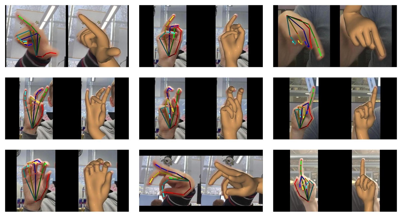
Sample GHUM hand fittings for hand images with 2D keypoint annotations overlaid. The data was used to train and test a variety of poses leading to better results for more extreme poses.

Model quality

In this new release, we substantially improved the quality of models, and evaluated them on a dataset of American Sign Language (ASL) gestures. As evaluation metric for 2D screen coordinates, we used Mean Average Precision (mAP) suggested by the COCO keypoint challenge methodology.

Hand model evaluation on American Sign Language dataset

For 3D evaluation we used Mean Absolute Error in Euclidean 3D metric space, with the average error measured in centimeters.

Model Name

2D, mAP, %

3D, mean 3D error, cm

HandPose GHUM Lite

79.2

1.4

HandPose GHUM Full

83.8

1.3

Previous TensorFlow.js HandPose

66.5

N/A

Quality metrics for newly released HandPose GHUM models vs. previously released TensorFlow.js HandPose model in for 2D and 3D predictions

Browser performance

We benchmark the model across multiple devices. All the benchmarks are tested with two hands presented.

MacBook Pro 15” 2019. 

Intel core i9. 

AMD Radeon Pro Vega 20 Graphics.

(FPS)

iPhone 11

(FPS)

Pixel 5

(FPS)

Desktop 

Intel i9-10900K. Nvidia GTX 1070 GPU.

(FPS)

MediaPipe Runtime

With WASM & GPU Accel.

62 | 48

8 | 5

19 | 15 

  136 | 120

TensorFlow.js Runtime
With WebGL backend

36 | 31

15 | 12

11 | 8 

 42 | 35 

Inference speed of HandPose across different devices and runtimes. The first number in each cell is for the lite model, and the second number is for the full model.

To see the model’s FPS on your device, try our demo. You can switch the model type and runtime live in the demo UI to see what works best for your device.

Cross platform availability

In addition to the JavaScript hand pose detection API, these updated hand models are also available in MediaPipe Hands as a ready-to-use Android Solution API and Python Solution API, with prebuilt packages in Android Maven Repository and Python PyPI respectively.

For instance, for Android developers the Maven package can be easily integrated into an Android Studio project by adding the following into the project’s Gradle dependencies:

dependencies {
implementation 'com.google.mediapipe:solution-core:latest.release'
implementation 'com.google.mediapipe:hands:latest.release'
}

The MediaPipe Android Solution is designed to handle different use scenarios such as processing live camera feeds, video files, as well as static images. It also comes with utilities to facilitate overlaying the output landmarks onto either CPU images (with Canvas) or GPU (using OpenGL). For instance, the following code snippet demonstrates how it can be used to process a live camera feed and render the output on screen in real-time:

// Creates MediaPipe Hands.
HandsOptions handsOptions =
HandsOptions.builder()
.setModelComplexity(1)
.setMaxNumHands(2)
.setRunOnGpu(true)
.build();
Hands hands = new Hands(activity, handsOptions);

// Connects MediaPipe Hands to camera.
CameraInput cameraInput = new CameraInput(activity);
cameraInput.setNewFrameListener(textureFrame -> hands.send(textureFrame));

// Registers a result listener.
hands.setResultListener(
handsResult -> {
handsView.setRenderData(handsResult);
handsView.requestRender();
})

// Starts the camera to feed data to MediaPipe Hands.
handsView.post(this::startCamera);

To learn more about MediaPipe Android Solutions, please refer to our documentation and try them out with the example Android Studio project. Also visit MediaPipe Solutions for more cross-platform solutions.

Acknowledgements

We would like to acknowledge our colleagues who participated in or sponsored creating HandPose GHUM 3D and building the APIs: Cristian Sminchisescu, Michael Hays, Na Li, Ping Yu, George Sung, Jonathan Baccash‎, Esha Uboweja, David Tian, Kanstantsin Sokal‎, Gregory Karpiak, Tyler Mullen, Chuo-Ling Chang, Matthias Grundmann.

Read More