All posts by : admin

Posted by Sayak Paul (MLE at Carted, and GDE) and Morgan Roff (Google)

We’re happy to share the work completed by Google Summer of Code students working with TensorFlow Hub this year. If you’re a student who is interested in writing open source code, then you’ll likely be interested in Google’s Summer of Code program.

Through this program, students propose project ideas to open source organizations, and if selected, receive a stipend to work with them to complete their projects over the summer. Students have the opportunity to learn directly from mentors within their selected organization, and organizations benefit from the students’ contributions. This year, 17 successful students completed their projects with the TensorFlow organization on many projects. In this article, we’ll focus on some of the work completed on TensorFlow Hub.

We’re Sayak and Morgan, two mentors for projects on TensorFlow Hub (TF Hub). Here we share what the students learned about building and publishing state-of-the-art models, training them on large-scale benchmark datasets, what we learned as mentors, and how rewarding summer of code was for each of us, and for the community.

We had the opportunity to mentor two students – Aditya Kane and Vasudev Gupta. Aditya successfully implemented several variants of RegNets including one based on this paper, and trained them on the ImageNet-1k dataset. Vasudev ported the pre-trained wav2vec2 weights from this paper to TensorFlow, which required him to implement the model architecture from scratch. He then demonstrated fine-tuning these pre-trained checkpoints on the LibriSpeech dataset, making his work more customizable and relevant for the community.

With model training happening at such a large scale, it becomes especially important to follow good engineering practices during the implementation. These include code modularization, unit tests, good design patterns, optimizations, and so on. Models were trained on Cloud TPUs to accelerate training time, and as such, substantial effort was put into the data input pipelines to ensure maximum accelerator utilization.

All of these factors collectively contributed to the complexity of the projects. Thanks to the Summer of Code program, students have the opportunity to tackle these challenges with the help of experienced mentors. This also enables students to gain insight into their organizations, and interact with people with many skillsets who cooperate to make large projects possible. A big thank you here to our students, who gracefully handled this engineering work and listened to our feedback.

Vasudev and Aditya contributed significant pre-trained models to TensorFlow Hub, along with tutorials (Wav2Vec, RegNetY) on their use, and TensorFlow implementations for folks who want to dig deeper. In their own words:

The last 2-3 months were full of lots of learning and coding. GSoC helped me get into the speech domain and motivated me to explore more about the TensorFlow ecosystem. I am thankful to my mentors for their continuous & timely feedback. I am looking forward to contributing more to the TensorFlow community and other awesome open source projects out there. – Vasudev Gupta

More about RegNets and Wav2Vec2

Almost 6 years after they were first published, ResNets are still widely used as benchmark architectures across image understanding tasks. Many recent self-supervised and semi-supervised learning frameworks still leverage ResNet50 as their backbone architectures. However, ResNets often do not scale well under larger data regimes and suffer from large training and inference time latencies as they grow. In contrast, RegNets were developed specifically to be a scalable architecture framework that maintains low latency while demonstrating high performance on standard image recognition tasks. Aditya’s models are published on TF Hub, with code and tutorials on GitHub.

Self-supervised learning is an important area of machine learning research. Many recent success stories have been focused on NLP and Computer Vision, and for Vasudev’s project, we wanted to explore speech. Last year, a group of researchers released the wav2vec2 framework for learning representations from audio in a self-supervised manner, benefiting downstream tasks like speech-to-text.

Using wav2vec2, you can now pre-train speech models without labeled data, and fine-tune those models on downstream tasks like speaker recognition. Vasudev’s models are available on TF Hub, along with a new tutorial on fine-tuning, and code on GitHub.

Wrapping up

We’d like to say a heartfelt thank you to all the students, mentors, and organizers who made Summer of Code a success despite this year’s many challenges. We encourage you to check out these models and share what you have built with us by tagging #TFHub on your social media posts, or share your work for the community spotlight program. If you have questions or want to learn more about these new models, you can ask them on discuss.tensorflow.org.

Read More

Posted by Gal Moran, Iris Shmuel, and Daniel Marcous (Data Scientists at Waze)

Waze

Waze is the world’s largest community-based traffic and navigation app. It uses real-time data to help users circumvent literal and figurative bumps in the road. On top of mobile navigation, Waze offers a web platform, a carpool app, partnership services, an advertisement platform and more. Such a broad portfolio brings along diverse technological challenges and many different use cases.

ML @Waze

Waze relies on many ML solutions, including:

• Predicting ETA
• Matching Riders & Drivers (Carpool)
• Serving The Right Ads

But it’s not that easy to get something like these right and “production grade”. It is very common for these kinds of projects to have requirements for complex surrounding infrastructure for getting them to production and hence require multiple engineers (data scientist, software engineer and software reliability engineers) and a lot of time. Even more so when you mix in the Waze-y requirements like large scale data, low (real-time, actually) latency inference, diverse use cases, and a whole lot of geospatial data.

The above is a good reason why opportunistically starting to do ML created a chaotic state at Waze. For us it manifested as:

• Multiple ML frameworks – you name it (sklearn, xgboost, TensorFlow, fbprophet, Java PMML, hand made etc.)
• ML & Ops disconnect – models & feature engineering embedded in (Java) backend servers by engineers with limited monitoring and validation capabilities
• Semi-manual operations for training, validation and deployment
• A hideously long development cycle from idea to production

Overall, data scientists ended up spending a lot of their time on ops and monitoring instead of focusing on the actual modelling and data processing. At a certain level of growth we’ve decided to organize the chaos and invest in automation and processes so we can scale faster. We’ve decided to heavily invest in a way to dramatically increase velocity and quality by adopting a full cycle data science philosophy. This means that in this new world we wanted to build, a single data scientist is able to close the product cycle from research to a production grade service.

Data scientists now directly contribute to production to maximize impact. They focus on modelling and data processing and get many infrastructures and ops work out-of-the-box. While we are not yet at the end of this journey fully realizing the above vision, we feel like the effort layed out here was crucial in putting us on the right track.

Waze’s ML Stack

Translating the above philosophy to a tech spec, we were set on creating an easy, stable, automated and uniform way of building ML pipelines at Waze.

Deep diving into tech requirements we came up with the below criteria:

• Simple — to understand, use, operate
• Managed — no servers, no hardware, just code
• Customizable — get the simple stuff for free, yet flexible enough to go crazy for the 5% that would require going outside the lines
• Scalable — auto scalable data processing, training, inference
• Pythonic — we need something production-ready, that works with most tools and code today and fits the standard data scientist. There are practically no other options than Python these days.

For the above reasons we’ve landed on TFX and the power of its built-in components to deliver these capabilities mostly out of the box.

It’s worth saying – Waze runs its tech stack on Google Cloud Platform (GCP).

It happens to be that GCP offers a suite of tools called Vertex AI. It is the ML infrastructure platform Waze is building on top of. While we use many components of Vertex AI’s managed services, we will focus here on – Vertex Pipelines – a framework for ML pipelines that helps us encapsulate TFX (or any pipeline) complexity and setup.

Together with our data tech stack, the overall ML architecture at Waze (all managed, scaled, pythonic etc.) is as follows:

Careful readers will notice the alleged caveat here – we go all in on TensorFlow.

TFX means TensorFlow (even though that’s not exactly true anymore, let’s assume it is).

It might be a little scary at first when you have many different use cases.

Fortunately, the TF ecosystem is rich and Waze has the merit of having large enough data that neural nets converge.

Since starting this we’ve yet to find a use case that TF magic does not solve better or adequately as other frameworks (and not talking about micro % points, not trying to do a Kaggle competition here but get something to production).

Waze TFX

You might think that landing on TFX and Vertex Pipelines solved all our problems, but that’s not exactly true.

In order to make things truly simple we’ve had to write some “glue code” (integrating the various products in the above architecture diagram) and abstracting enough details so the common data scientist could use this stuff effectively and fast.

That resulted in:

• Eliminated boilerplate
• Hiding all common TFX components so data scientists only focus on feature engineering and modelling and get the entire pipeline for free
• Generating BigQuery based train / eval split
• Providing pre-implemented optional common features transform (e.g. scaling, normalization, imputations)
• Providing pre-implemented Keras models (e.g. DNN/RNN model. TF Estimator like but in Keras that speaks TFX)
• Utility functions (e.g. TF columns preparation)
• Unit testing framework for tf.transform feature engineering code
• Orchestrated and scheduled pipeline runs from Airflow using a Cloud run instance with all TFX packages installed (without installing it on the Airflow composer)

We’ve put it all in an easy to use Python package called “waze-data-tfx”

On top, we provided a super detailed walkthrough, usage guides and code templates, to our data scientists, so the common DS workflow is: fork, change config, tweak the code a little, deploy.

For reference this is how a simple waze-data-tfx pipeline looks like:

1. Configuration

   _DATASET_NAME = 'tfx_examples'
   _TABLE_NAME = 'simple_template_data'
   
   _LABEL_KEY = 'label'
   _CATEGORICAL_INT_FEATURES = {
      "categorical_calculated": 2,
   }
   _DENSE_FLOAT_FEATURE_KEYS = ["numeric_feature1", "numeric_feature2"]
   _BUCKET_FEATURES = {
      "numeric_feature1": 5,
   }
   _VOCAB_FEATURES = {
      "categorical_feature": {
          'top_k': 5,
          'num_oov_buckets': 3
      }
   }
   
   _TRAIN_BATCH_SIZE = 128
   _EVAL_BATCH_SIZE = 128
   _NUM_EPOCHS = 250
   
   _TRAINING_ARGS = {
      'dnn_hidden_units': [6, 3],
      'optimizer': tf.keras.optimizers.Adam,
      'optimizer_kwargs': {
          'learning_rate': 0.01
      },
      'layer_activation': None,
      'metrics': ["Accuracy"]
   }
   
   _EVAL_METRIC_SPEC = create_metric_spec([
      mse_metric(upper_bound=25, absolute_change=1),
      accuracy_metric()
   ])

2. Feature Engineering

   def preprocessing_fn(inputs):
      """tf.transform's callback function for preprocessing inputs.
   
      Args:
          inputs: map from feature keys to raw not-yet-transformedfeatures.
   
      Returns:
          Map from string feature key to transformed feature operations.
      """
      outputs = features_transform(
          inputs=inputs,
          label_key=_LABEL_KEY,
          dense_features=_DENSE_FLOAT_FEATURE_KEYS,
          vocab_features=_VOCAB_FEATURES,
          bucket_features=_BUCKET_FEATURES,
      )
      return outputs

3. Modelling

   def _build_keras_model(**training_args):
      """Build a keras model.
   
      Args:
          hidden_units: [int], the layer sizes of the DNN (input layer first).
          learning_rate: [float], learning rate of the Adam optimizer.
   
      Returns:
          A keras model
      """
      feature_columns = 
          prepare_feature_columns(
              dense_features=_DENSE_FLOAT_FEATURE_KEYS,
              vocab_features=_VOCAB_FEATURES,
              bucket_features=_BUCKET_FEATURES,
          )
   
      return _dnn_regressor(deep_columns=list(feature_columns.values()),
                            dnn_hidden_units=training_args.get(
                                "dnn_hidden_units"),
                            dense_features=_DENSE_FLOAT_FEATURE_KEYS,
                            vocab_features=_VOCAB_FEATURES,
                            bucket_features=_BUCKET_FEATURES,
                            )

4. Orchestration

   pipeline_run = WazeTFXPipelineOperator(
      dag=dag,
      task_id='pipeline_run',
      model_name='basic_pipeline_template',
      package=tfx_pipeline_basic,
      pipeline_project_id=EnvConfig.get_value('gcp-project-infra'),
      table_project_id=EnvConfig.get_value('gcp-project-infra'),
      project_utils_filename='utils.py',
      gcp_conn_id=gcp_conn_id,
      enable_pusher=True,
   )

Simple, right?

When you commit a configuration file to the code base it gets deployed and sets up continuous training, and a full blown pipeline including all TFX and Vertex AI magics like data validation, transforms deployed to Dataflow, monitoring etc.

Summary

We knew we were up to something good when one of our data scientists came back from a long leave and had to use this new framework for a use case. She said that she was able to spin up a full production-ready pipeline in hours, something that before her leave would have taken her weeks to do.

Going forward we have much planned that we want to bake into `waze-data-tfx`. A key advantage that we see in having this common infrastructure is that once a feature is added, then everyone can enjoy it “for free”. For example, we plan on adding additional components to the pipeline, such as Infra Validator and Fairness Indicators. Once these are supported, every new or existing ML pipeline will add these components out-of-the-box, no extra code needed.

Additional improvements we are planning are around deployment. We wish to provide deployment quality assurance while automating as much as possible.

One way we are currently exploring doing so is using canary deployments. A data scientist will simply need to configure an evaluation metric and the framework (using Vertex Prediction traffic splitting capabilities and other continuous evaluation magic) would test the new model in production and gradually deploy or rollback according to the evaluated metrics.

Read More

Posted by Elie Bursztein and Owen Vallis, Google

Today we are releasing the first version of TensorFlow Similarity, a python package designed to make it easy and fast to train similarity models using TensorFlow.

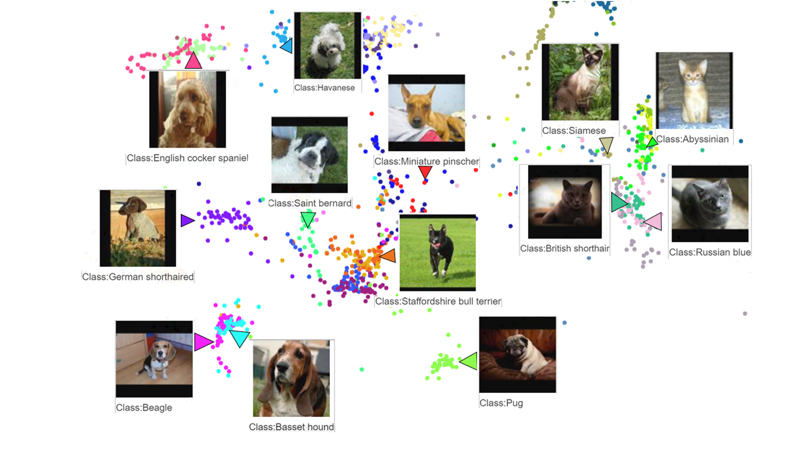
Examples of nearest neighbor searches performed on the embeddings generated by a similarity model trained on the Oxford IIIT Pet Dataset

The ability to search for related items has many real world applications, from finding similar looking clothes, to identifying the song that is currently playing, to helping rescue missing pets. More generally, being able to quickly retrieve related items is a vital part of many core information systems such as multimedia searches, recommender systems, and clustering pipelines.

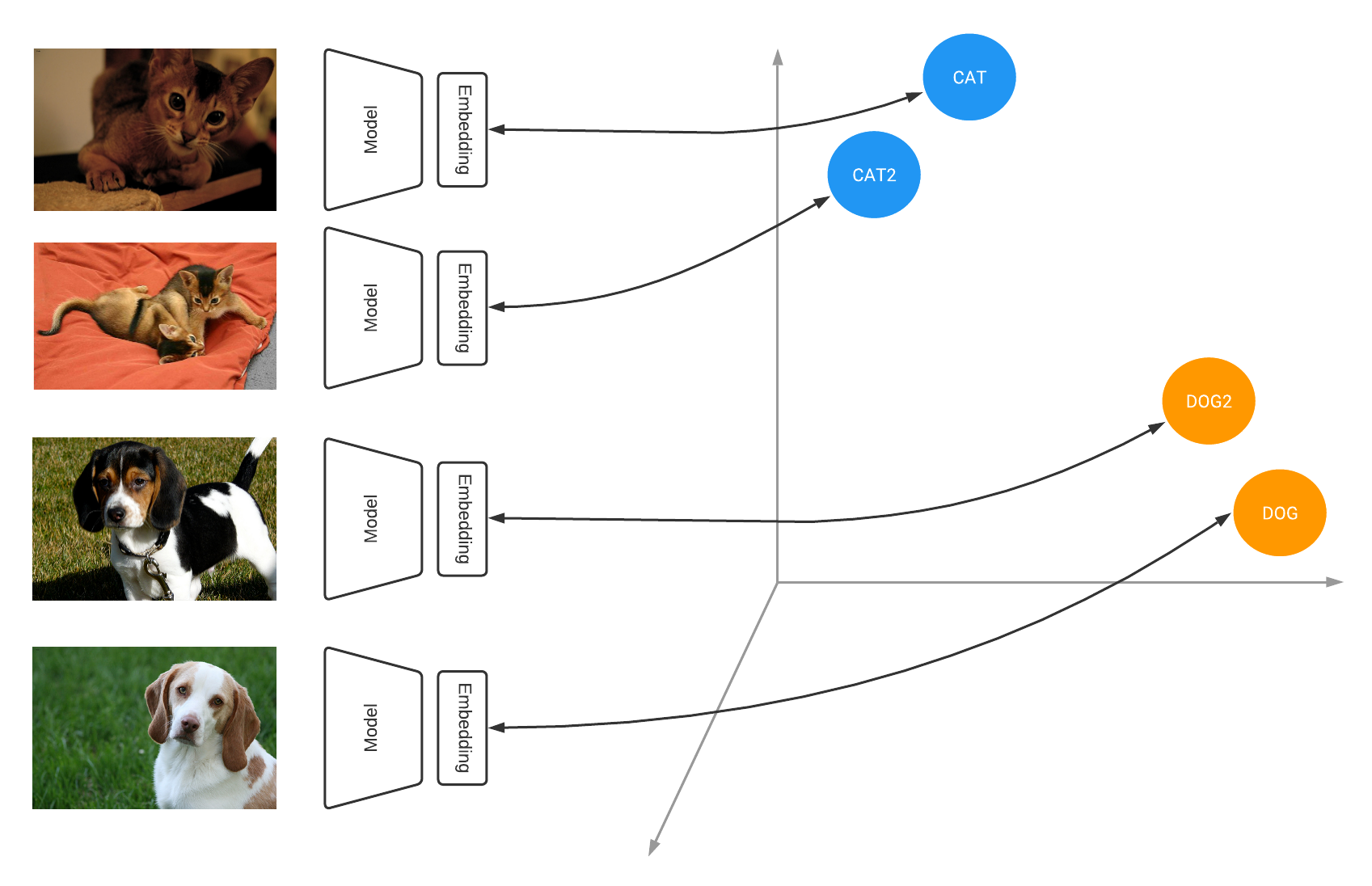Similarity models learn to output embeddings that project items in a metric space where similar items are close together and far from dissimilar ones

Under the hood, many of these systems are powered by deep learning models that are trained using contrastive learning. Contrastive learning teaches the model to learn an embedding space in which similar examples are close while dissimilar ones are far apart, e.g., images belonging to the same class are pulled together, while distinct classes are pushed apart from each other. In our example, all the images from the same animal breed are pulled together while different breeds are pushed apart from each other.

Oxford-IIIT Pet dataset visualization using the Tensorflow Similarity projector

When applied to an entire dataset, contrastive losses allow a model to learn how to project items into the embedding space such that the distances between embeddings are representative of how similar the input examples are. At the end of training you end up with a well clustered space where the distance between similar items is small and the distance between dissimilar items is large. For example, as visible above, training a similarity model on the Oxford-IIIT Pet dataset leads to meaningful clusters where similar looking breeds are close-by and cats and dogs are clearly separated.

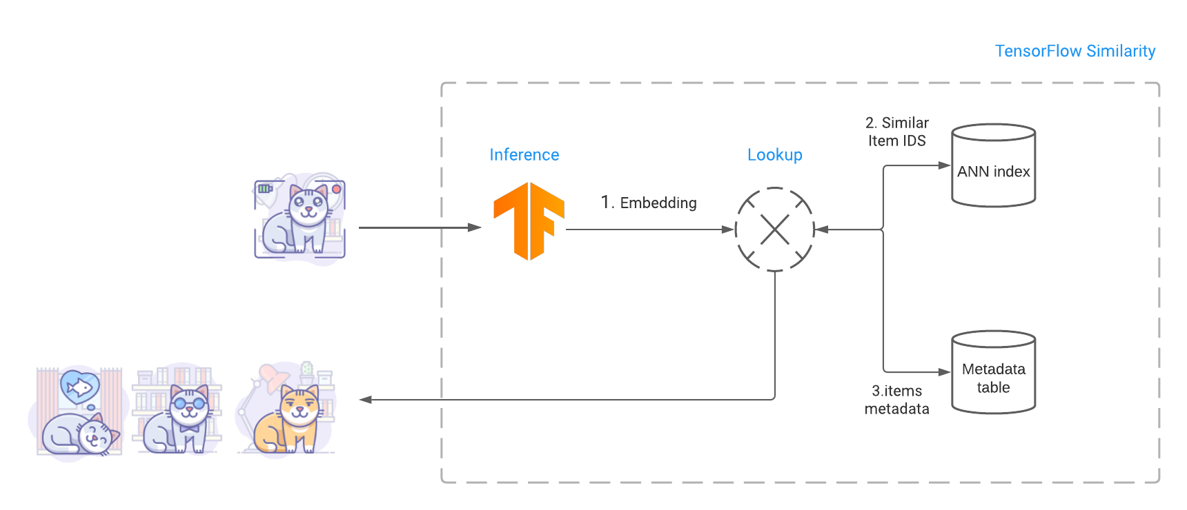Finding related items involve computing the query image embedding, performing an ANN search to find similar items and fetching similar items metadata including the images bytes.

Once the model is trained, we build an index that contains the embeddings of the various items we want to make searchable. Then at query time, TensorFlow Similarity leverages Fast Approximate Nearest Neighbor search (ANN) to retrieve the closest matching items from the index in sub-linear time. This fast look up leverages the fact that TensorFlow Similarity learns a metric embedding space where the distance between embedded points is a function of a valid distance metric. These distance metrics satisfy the triangle inequality, making the space amenable to Approximate Nearest Neighbor search and leading to high retrieval accuracy.

Other approaches, such as using model feature extraction, require the use of an exact nearest neighbor search to find related items and may not be as accurate as a trained similarity model. This prevents those methods scaling as performing an exact search requires a quadratic time in the size of the search index. In contrast, TensorFlow Similarity’s built-in Approximate Nearest Neighbor indexing system, which relies on the NMSLIB, makes it possible to search over millions of indexed items, retrieving the top-K similar matches within a fraction of second.

Beside accuracy and retrieval speed, the other major advantage of similarity models is that they allow you to add an unlimited new number of classes to the index without having to retrain. Instead you only need to compute the embeddings for representative items of the new classes and add them to the index. This ability to dynamically add new classes is particularly useful when tackling problems where the number of distinct items is unknown ahead of time, constantly changing, or is extremely large. An example of this would be enabling users to discover newly released music that is similar to songs they have liked in the past.

TensorFlow Similarity provides all the necessary components to make similarity training evaluation and querying intuitive and easy. In particular, as illustrated below, TensorFlow Similarity introduces the SimilarityModel(), a new Keras model that natively supports embedding indexing and querying. This allows you to perform end-to-end training and evaluation quickly and efficiently..

A minimal example that trains, indexes and searches on MNIST data can be written in less than 20 lines of code:

from tensorflow.keras import layers

# Embedding output layer with L2 norm
from tensorflow_similarity.layers import MetricEmbedding 
# Specialized metric loss
from tensorflow_similarity.losses import MultiSimilarityLoss 
# Sub classed keras Model with support for indexing
from tensorflow_similarity.models import SimilarityModel
# Data sampler that pulls datasets directly from tf dataset catalog
from tensorflow_similarity.samplers import TFDatasetMultiShotMemorySampler
# Nearest neighbor visualizer
from tensorflow_similarity.visualization import viz_neigbors_imgs


# Data sampler that generates balanced batches from MNIST dataset
sampler = TFDatasetMultiShotMemorySampler(dataset_name='mnist', classes_per_batch=10)

# Build a Similarity model using standard Keras layers
inputs = layers.Input(shape=(28, 28, 1))
x = layers.Rescaling(1/255)(inputs)
x = layers.Conv2D(64, 3, activation='relu')(x)
x = layers.Flatten()(x)
x = layers.Dense(64, activation='relu')(x)
outputs = MetricEmbedding(64)(x)

# Build a specialized Similarity model
model = SimilarityModel(inputs, outputs)

# Train Similarity model using contrastive loss
model.compile('adam', loss=MultiSimilarityLoss())
model.fit(sampler, epochs=5)

# Index 100 embedded MNIST examples to make them searchable
sx, sy = sampler.get_slice(0,100)
model.index(x=sx, y=sy, data=sx)

# Find the top 5 most similar indexed MNIST examples for a given example
qx, qy = sampler.get_slice(3713, 1)
nns = model.single_lookup(qx[0])

# Visualize the query example and its top 5 neighbors
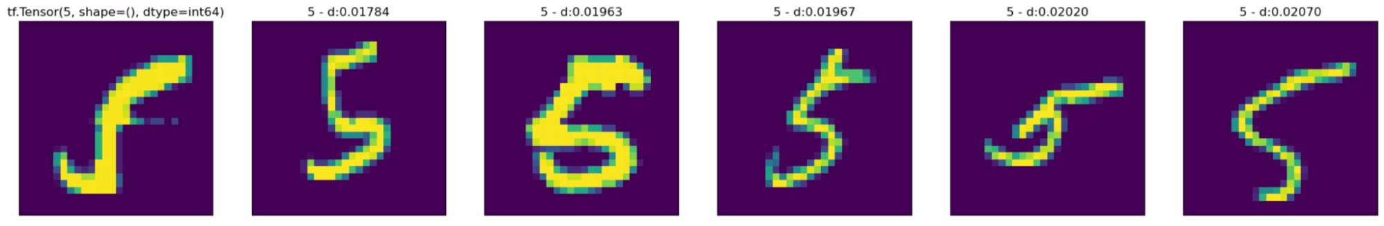
viz_neigbors_imgs(qx[0], qy[0], nns)

Even though the code snippet above uses a sub-optimal model, it still yields good matching results where the nearest neighbors clearly looks like the queried digit as visible in the screenshot below:

This initial release focuses on providing all the necessary components to help you build contrastive learning based similarity models, such as losses, indexing, batch samplers, metrics, and tutorials. TF Similarity also makes it easy to work with the Keras APIs and use the existing Keras Architectures. Moving forward, we plan to build on this solid foundation to support semi-supervised and self-supervised methods such as BYOL, SWAV, and SimCLR.

You can start experimenting with TF Similarity right away by heading to the Hello World tutorial. For more information you can check out the project Github.

Read More

Posted by Marat Dukhan and Frank Barchard, software engineers

Quantization is among the most popular methods to speedup neural network inference on CPUs. A year ago TensorFlow Lite increased performance for floating-point models with the integration of XNNPACK backend. Today, we are extending the XNNPACK backend to quantized models with, on average across computer vision models, 30% speedup on ARM64 mobile phones, 5X speedup on x86-64 laptop and desktop systems, and 20X speedup for in-browser inference with WebAssembly SIMD compared to the default TensorFlow Lite quantized kernels.

Quantized inference in XNNPACK is optimized for symmetric quantization schemas used by the TensorFlow Model Optimization Toolkit. XNNPACK supports both the traditional per-tensor quantization schema and the newer accuracy-optimized schema with per-channel quantization of weights and per-tensor quantization of activations. Additionally, XNNPACK supports the asymmetric quantization schema, albeit with reduced efficiency.

Performance improvements

We evaluated XNNPACK-acclerated quantized inference on a number of edge devices and neural network architectures. Below, we present benchmarks on four public and two internal quantized models covering common computer vision tasks:

1. EfficientNet-Lite0 image classification [download]
2. EfficientDet-Lite0 object detection [download]
3. DeepLab v3 segmentation with MobileNet v2 feature extractor [download]
4. CartoonGAN image style transfer [download]
5. Quantized version of the Face Mesh landmarks
6. Quantized version of the Video Segmentation

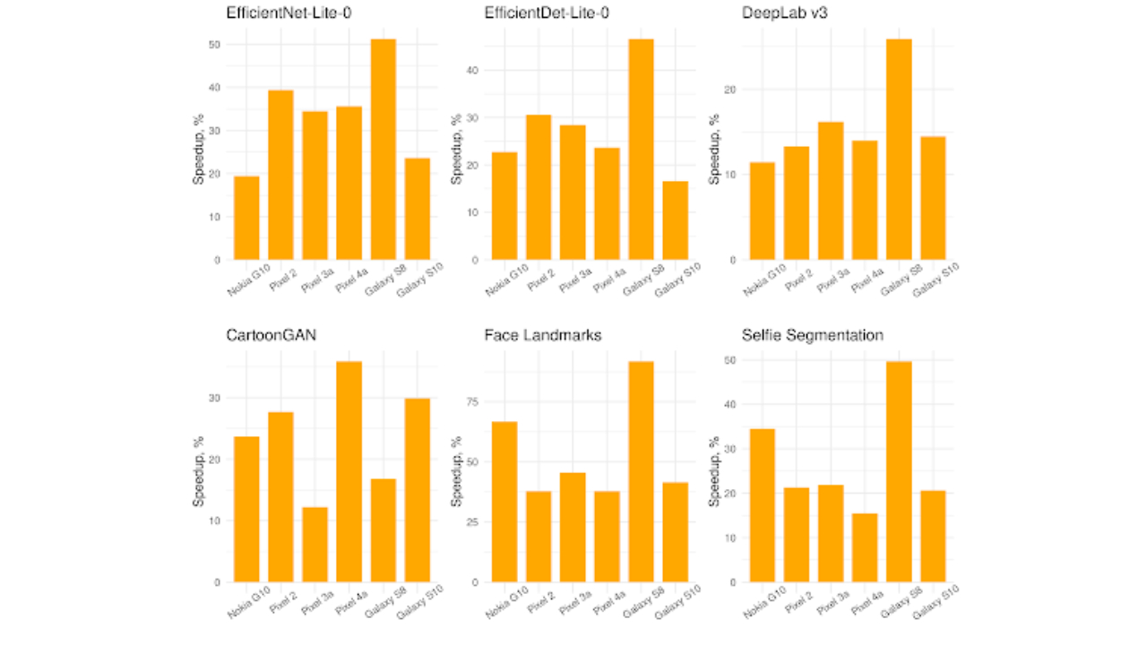
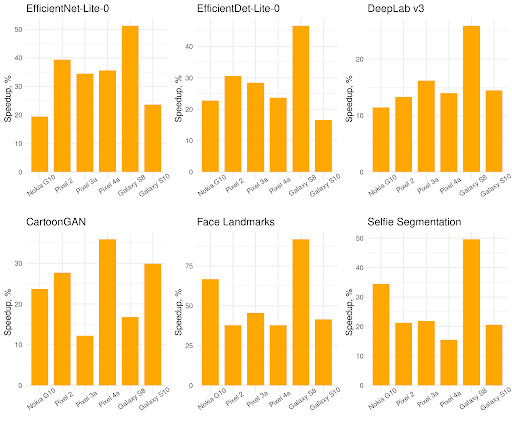Speedup from XNNPACK on single-threaded inference of quantized computer vision models on Android/ARM64 mobile phones.

Across the six Android ARM64 mobile devices XNNPACK delivers, on average, 30% speedup over the default TensorFlow Lite quantized kernels.

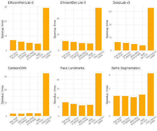Speedup from XNNPACK on single-threaded inference of quantized computer vision models on x86-64 laptop and desktop systems.

XNNPACK offers even greater improvements on laptop and desktop systems with x86 processors. On the 5 x86 processors in our benchmarks XNNPACK accelerated inference on average by 5 times. Notably, low-end and older processors which don’t support AVX instructions see over 20X speedup from switching quantized inference to XNNPACK: while the previous TensorFlow Lite inference backend had optimized implementations only for AVX, AVX2, and AVX512 instruction sets, XNNPACK provides optimized implementations for all x86-64 processors.

Speedup from XNNPACK on single-threaded WebAssembly SIMD inference of quantized computer vision models on mobile phones, laptops, and desktops when running through V8.

Besides the traditional mobile and laptop/desktop platforms, XNNPACK brings accelerated quantized inference to the Web platform through the TensorFlow Lite Web API. The above plot demonstrates a geomean speedup of 20X over the default TensorFlow Lite implementation when running WebAssembly SIMD benchmarks through the V8 JavaScript engine on 3 x86-64 and 2 ARM64 systems.

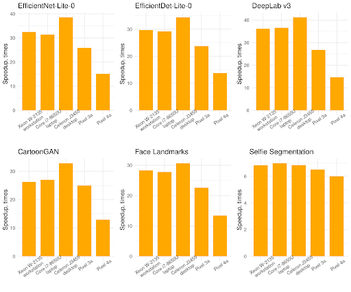
Two years of optimizations

XNNPACK started its life as a fork of QNNPACK library, but as the first version of XNNPACK focused on floating-point inference and QNNPACK focused on quantized inference, it was not possible to compare the two. Now with XNNPACK introducing support for quantized inference, we can directly evaluate and attribute the two further years of performance optimizations.

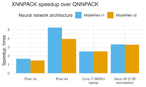
To compare the two quantized inference backends, we ported randomized MobileNet v1 and MobileNet v2 models from XNNPACK API to QNNPACK API, and benchmarked their single-threaded performance on two ARM64 Android phones and two x86-64 systems. The results are presented in the plot above, and the progress made by XNNPACK in two years is striking. XNNPACK is 50% faster on the older Pixel 3a phone and 4-5X faster on the newer Pixel 4a phone, 2.5X faster on the x86-64 laptop, and over 3X faster on the x86-64 workstation. These improvements are the result of a multiple optimizations XNNPACK gained in the two years since it forked from QNNPACK:

• XNNPACK retained the optimizations in QNNPACK, like the Indirect Convolution algorithm and microarchitecture-specific microkernel selection, and further augmented them with Indirect Deconvolution algorithm, and more flexible capabilities, like built-in numpy-like broadcasting in the quantized addition and quantized multiplication operators.
• Convolution, Deconvolution, and Fully Connected operators accumulate products of 8-bit activations and weights into a 32-bit number, and in the end this number needs to be converted back, or requantized, to an 8-bit number. There are multiple ways how requantization can be implemented, but QNNPACK adapted schema from the GEMMLOWP library, which pioneered quantized computations for neural network inference. However, it has since been discovered that GEMMLOWP requantization schema is suboptimal in terms of both accuracy and performance, and XNNPACK replaced it with more performant and accurate alternatives
• Whereas QNNPACK targeted asymmetric quantization schema, where both activations and weights are represented as unsigned integers with zero point and scale quantization parameters, XNNPACK’s optimizations focus on symmetric quantization, where both activations and weights are signed integers, and weights have additional restrictions: the zero point of the weights is always zero and the quantized weights elements are limited to the [-127, 127] range (-128 is excluded even though it can be represented as a signed 8-bit integer). Symmetric quantization offers two computational advantages exploited in XNNPACK. First, when the filter weights are static, the results of accumulating the product of input zero point by the filter weights can be completely fused into the bias term in the Convolution, Deconvolution, and Fully Connected operators. Thus, zero point parameters are completely absent from the inference computations. Secondly, the product of a signed 8-bit input element by the weight element restricted to [-127, 127] fits into 15 bits. This enables the microkernels for Convolution, Deconvolution, and Fully Connected operators to do half of the accumulations on 16-bit variables rather than always extending the products to 32 bits.
• QNNPACK microkernels were optimized NEON SIMD instructions on ARM and SSE2 SIMD instructions on x86, but XNNPACK supports a much wider set of instruction set-specific optimizations. Most quantized microkernels in XNNPACK are optimized for SSE2, SSE4.1, AVX, XOP, AVX2, and AVX512 instructions on x86/x86-64, for NEON, NEON V8, and NEON dot product instructions on ARM/ARM64, and for WebAssembly SIMD instructions. Additionally, XNNPACK provides scalar implementations for WebAssembly 1.0 and pre-NEON ARM processors.
• QNNPACK introduced the idea of specialized assembly microkernels for high-end ARM and low-end ARM cores, but XNNPACK takes this idea much further. XNNPACK not only includes specialized expert-tuned software pipelined assembly microkernels for Cortex-A53, Cortex-A55, and high-end cores with and without NEON dot product instructions, but even supports switching between them on the fly. When a thread doing inference migrates from a big to a little core, XNNPACK automatically adapts from using a microkernel optimized for the big core to the one optimized for the little core.
• QNNPACK mainly focused on multi-threaded inference and organized computations as a large number of small tasks, each computing a tiny tile of the output tensor. XNNPACK reworked parallelisation and made the tasks flexible: they can be fine-grained or coarse-grained depending on the number of threads participating in the parallelization. Through dynamic adjustment of task granularity, XNNPACK archives low overhead in single-threaded execution and high parallelization efficiency for multi-threaded inference.

Taken together, these optimizations make XNNPACK the new state-of-art for quantized inference, and turn TensorFlow Lite into the most versatile quantized inference solution, covering systems from Raspberry Pi Zero to Chromebooks to workstations with server-class processors.

How can you use it?

Quantized XNNPACK inference is enabled by default in the CMake builds of TensorFlow Lite for all platforms, in the Bazel builds of TensorFlow Lite for the Web platform, and will be available in TensorFlow Lite Web API in the 2.7 release. In Bazel builds for other platforms, quantized XNNPACK inference is enabled via a build-time opt-in mechanism. When building TensorFlow Lite with Bazel, add --define tflite_with_xnnpack=true --define xnn_enable_qs8=true, and the TensorFlow Lite interpreter will use the XNNPACK backend by default for supported operators with symmetric quantization. Limited support for operators with asymmetric quantization is available via the --define xnn_enable_qu8=true Bazel option.

Which operations are accelerated?

The XNNPACK backend currently supports a subset of quantized TensorFlow Lite operators (see documentation for details and limitations). XNNPACK supports models produced by the Model Optimization Toolkit through post-training integer quantization and quantization-aware training, but not post-training dynamic range quantization.

Future work

This is the third version of the XNNPACK integration into TensorFlow Lite following the initial release of the floating-point implementation and the subsequent release that brought sparse inference support. In the following versions we plan to add the following improvements:

• Half-precision inference on the recent ARM processors
• Sparse quantized inference.
• Even faster dense inference.

We encourage you to leave your thoughts and comments on our GitHub and StackOverflow pages, and you can ask questions on discuss.tensorflow.org

Read More