Better Than 8K Resolution: NVIDIA Inception Displays Global AI Startup Ecosystem

There are more AI startups in healthcare than any other single industry. The number of AI startups in media and entertainment is about the same as that in retail. More than one in 10 of all AI startups is based in California.

How do we know this? NVIDIA Inception, our acceleration platform for AI startups, has now surpassed 8,500 members. That’s about two-thirds of the total number of AI startups worldwide, as estimated by Pitchbook. With total cumulative funding of over $60 billion and members in 90 countries, NVIDIA Inception is one of the largest AI startup ecosystems in the world.

With this type of scale, NVIDIA Inception is more than a singular program; it’s a reflection of the larger startup landscape. And there’s plenty that can be inferred based on this.

Data Across 8,500+ Startups

NVIDIA Inception figures show the United States leads the world in terms of both the number of AI startups, representing nearly 27 percent, and the amount of secured funding, accounting for over $27 billion in cumulative funding.

Of U.S.-based startups, 42 percent were based in California — more than one in 10 AI startups is based in the state — with 29 percent in the San Francisco Bay Area. This underscores the continued draw of the region for startup founders and VC funding.

Following the U.S. is China, in terms of both funding and company stage, with 12 percent of NVIDIA Inception members based there. India comes in third at 7 percent, with the United Kingdom right behind at 6 percent.

Taken together, AI startups based in the U.S., China, India and the U.K. account for just over half of all startups in NVIDIA Inception. Following in order after these are Germany, Russia, France, Sweden, Netherlands, Korea and Japan.

In terms of industries, healthcare, IT services, intelligent video analytics (IVA), media and entertainment (M&E) and robotics are the top five in NVIDIA Inception. AI startups in healthcare account for 16 percent of Inception members, followed by those in IT services at 15 percent. AI startups in IVA make up 8 percent, with M&E and robotics AI startups tied at 7 percent.

Details Spanning 3,000+ Startups Since 2020

More than 3,000 AI startups have joined NVIDIA Inception since 2020. Similar to data across Inception as a whole, AI startups from the U.S. account for the largest segment (27 percent), followed by China (12 percent), and India and the U.K. (tied at 6 percent).

Additionally, startups that have joined since 2020 are concentrated in the same top five industries, though in slightly different order. IT services leads the way at 17 percent, followed by healthcare at 16 percent, M&E at 9 percent, IVA at 8 percent and robotics at 5 percent.

Within the top two industries —  healthcare and IT services — there’s more detail among AI startups who have joined since 2020. The dominant segment within IT services is computer vision at 27 percent, with predictive analytics in second place at 9 percent. The top two segments in healthcare are medical analytics at 38 percent and medical imaging at 36 percent, though the fastest growth is among AI startups in the pharma and AI biology industries at 15 percent.

Virtual and augmented reality startup companies are far outpacing any other segment within M&E, mostly due to the pandemic. These startups are coming to NVIDIA Inception with a shared vision of building an ecosystem for the metaverse.

Disruption Through Startups 

Since Inception’s launch in 2016, it has grown more than tenfold. This growth has accelerated year over year, with membership increasing to 26 percent in 2020, and already reaching 17 percent in the first half of 2021.

NVIDIA Inception is a program built to accommodate and nurture every startup that is accelerating computing, at every stage in their journey. All program benefits are free of charge — there are no fees ever. And unlike other accelerators or incubators, startups never have to give up equity to join.

Startups are the single best lens into the future of modern AI, so join with us today by applying for NVIDIA Inception.

The post Better Than 8K Resolution: NVIDIA Inception Displays Global AI Startup Ecosystem appeared first on The Official NVIDIA Blog.

Read More

Stanford AI Lab Papers at ACL-IJCNLP 2021

The Joint Conference of the 59th Annual Meeting of the Association for Computational Linguistics and the 11th
International Joint Conference on Natural Language Processing
is being hosted virtually this week. We’re excited to share all the work from SAIL that’s being presented, and you’ll find links to papers, videos and blogs below. Feel free to reach out to the contact authors directly to learn more about the work that’s happening at Stanford!

List of Accepted Long Papers

Neural Event Semantics for Grounded Language Understanding


Authors: Shyamal Buch, Li Fei-Fei, Noah D. Goodman

Contact: shyamal@cs.stanford.edu

Links: Paper | Project Webpage

Keywords: grounded language, compositionality, modular networks, event semantics

Notes: Accepted as a paper to TACL 2021, presented at ACL-IJCNLP 2021!


Measuring Conversational Update: A Case Study on Student-Teacher Interactions


Authors: Dorottya Demszky, Jing Liu, Zid Mancenido, Julie Cohen, Heather Hill, Dan Jurafsky, Tatsunori Hashimoto

Contact: ddemszky@stanford.edu

Links: Paper | Code & Data

Keywords: conversational uptake, education


Mind Your Outliers! Investigating the Negative Impact of Outliers on Active Learning for Visual Question Answering


Authors: Siddharth Karamcheti, Ranjay Krishna, Li Fei-Fei, Christopher D. Manning

Contact: skaramcheti@cs.stanford.edu

Links: Paper | Code

Keywords: active learning, visual question answering, interpretability

Notes: Outstanding Paper Award


Relevance-guided Supervision for OpenQA with ColBERT


Authors: Omar Khattab, Christopher Potts, Matei Zaharia

Contact: okhattab@stanford.edu

Links: Paper | Code

Keywords: open-domain question answering, neural retrieval, weak supervision

Notes: Accepted as a paper to TACL 2021, presented at ACL-IJCNLP 2021!


Prefix Tuning: Optimizing Continuous Prompts for Generation


Authors: Xiang Lisa Li, Percy Liang

Contact: xlisali@stanford.edu

Links: Paper | Code

Keywords: prefix-tuning, fine-tuning for generation, large-scale fine-tuning


DynaSent: A Dynamic Benchmark for Sentiment Analysis


Authors: Christopher Potts*, Zhengxuan Wu*, Atticus Geiger, Douwe Kiela

Contact: cgpotts@stanford.edu

Links: Paper | Code | Video


Keywords: sentiment analysis, crowdsourcing, adversarial datasets


List of Accepted Short Papers

Attention Flows are Shapley Values


Authors: Kawin Ethyarajh, Dan Jurafsky

Contact: kawin@stanford.edu

Links: Paper

Keywords: explainability; interpretability


Question Generation for Adaptive Education


Authors: Megha Srivastava, Noah D. Goodman

Contact: meghas@stanford.edu

Links: Paper

Keywords: education, nlp, language generation


We look forward to seeing you at ACL-IJCNLP 2021!

Read More

A Unifying, Game-Theoretic Framework for Imitation Learning

Imitation learning (IL) is the problem of finding a policy, (pi), that is as close as possible to an expert’s policy, (pi_E). IL algorithms can be grouped broadly into (a) online, (b) offline, and (c) interactive methods. We provide, for each setting, performance bounds for learned policies that apply for all algorithms, provably efficient algorithmic templates for achieving said bounds, and practical realizations that out-perform recent work.

From beating the world champion at Go (Silver et al.) to getting cars to drive themselves (Bojarski et al.), we’ve seen unprecedented successes in learning to make sequential decisions over the last few years. When viewed from an algorithmic viewpoint, many of these accomplishments share a common paradigm: imitation learning (IL). In imitation learning, one is given access to samples of expert behavior (e.g. moves chosen by Monte-Carlo Tree Search or steering angles recorded from an expert driver) and tries to learn a policy that mimics this behavior. Unlike reinforcement learning, imitation learning does not require careful tuning of a reward function, making it easier to scale to real-world tasks where one is able to gather expert behavior (like Go or driving). As we continue to apply imitation learning algorithms to safety-critical problems, it becomes increasingly important for us to have strong guarantees on their performance: while wrong steps in Go lead to a lost game at worst, mistakes of self-driving cars could result in far worse. In our ICML’21 Paper Of Moments and Matching: A Game Theoretic Framework for Closing the Imitation Gap, we provide bounds on how well any imitation algorithm can do, as well as provably efficient algorithms for achieving these bounds.

A Taxonomy of Imitation Learning Algorithms

Let’s focus on the problem of trying to teach a car to drive around a track from expert demonstrations. We instrument the car with cameras and sensors that measure the angle of the wheel and how hard the pedals are being pushed. Then, in terms of increasing requirements, the approaches we could take are:

  • Offline: Have the expert drive laps, recording their states (camera images) and actions (pedals/wheel). Use your favorite supervised learning algorithm to regress from states to actions. This approach is called Behavioral Cloning.
  • Online: Record expert states and actions. Then, have the car try to drive around the track and measure the delta between learner and expert trajectories. Train the policy to minimize this delta. GAIL is an algorithm that uses a discriminator network to measure this delta.
  • Interactive: (0) Start with an empty dataset D. (1) Record the car driving a sample lap. (2) Ask the expert driver what they would have done for each recorded image. Append this data to D. (3) Regress over data in D. (4) Go back to 1. This approach is known as DAgger.

One of our key insights is that all three of these approaches can be seen as minimizing a sort of divergence from expert behavior. Concretely,

  • Offline: We measure a divergence between learner and expert actions on states from expert demonstrations.
  • Online: We measure a divergence between learner and expert trajectories.
  • Interactive: We measure a divergence between learner and expert actions but on states from learner rollouts.

Also notice that as we transition from Offline to Online IL, we add a requirement of access to the environment or an accurate simulator. As we move from Online to Interactive IL, we also need access to a queryable expert. Let (pi) denote the policy, (pi_E) denote the expert’s policy, and (f) denote the divergence. We can visualize our thoughts thus far as:

With this divergence-minimizing perspective in mind, we’re able to introduce a unifying, game-theoretic perspective.

A Game-Theoretic Perspective on IL

A natural question at this point might be: what divergence should one use to measure the difference between learner and expert behavior? Examples abound in the literature: Kullback-Liebler? Wasserstein? Jensen-Shannon? Total Variation? Maximum Mean Discrepancy? Without prior knowledge about the problem, it’s really hard to say. For example, KL Divergence has a mode-covering effect — this means that if half the data was the expert swerving left to avoid a tree and half the data was them swerving right, the learner would learn to pick a point in the middle and drive straight into the tree!

If we’re not sure what divergence is the right choice, we can just minimize all of them, which is equivalent to minimizing a worst-case or adversarially-chosen one. Using (pi) and (pi_E) to denote the learner and expert policies, we can write out the optimization problem for each setting:

  • Offline: $$ min_{pi} max_f mathbb{E}_{s, a sim pi_E}[f(s, pi(s)) – f(s, a)] $$
  • Online: $$ min_{pi} max_f mathbb{E}_{s, a sim pi}[f(s, a)] – mathbb{E}_{s, a sim pi_E}[f(s, a)]$$
  • Interactive: $$ min_{pi} max_f mathbb{E}_{s, a sim pi}[f(s, a) – f(s, pi_E(s))] $$

Each of these equations is in the form of a two-player zero-sum game between a learner (pi) and a discriminator (f). Two-player zero-sum games have been extensively studied in game theory, allowing us to use standard tools to analyze and solve them. Notice the similarity of the forms of these games — the only real difference is which state-action distributions the divergence is calculated between. Thus, we can view all three classes of imitation learning as solving a games with different classes of discriminators. This game-theoretic perspective is extremely powerful for a few reasons:

  1. As we have access to more information (e.g. a simulator or a queryable expert), we’re able to evaluate more powerful discriminators. Minimizing these more powerful discriminators leads to tighter performance bounds. Specifically, we show that the difference between learner and expert performance for offline IL scales quadratically with the horizon of the problem, and linearly for online / interactive IL. Quadratically compounding errors translate to poor real-world performance. Thus, one perspective on our bounds is that they show that access to a simulator or a queryable expert is both necessary and sufficient for learning performant policies. We recommend checking out the full paper for the precise upper and lower bounds.
  2. These performance bounds apply for all algorithms in each class — after all, you can’t do better by considering a more restrictive class of divergences. This means our bounds apply for a lot of prior work (e.g. Behavioral Cloning, GAIL, DAgger, MaxEnt IRL, …). Importantly, these bounds also apply for all non-adversarial algorithms: they’re just optimizing over a singleton discriminator class.
  3. Our game-theoretic perspective also tells us that finding a policy that minimizes the worst-case divergence is equivalent to finding a Nash Equilibrium of the corresponding game, a problem we know how to solve provably efficiently for two-player zero-sum games. By solving a particular game, we inherit the performance bounds that come with the class of divergences considered.

Together, these three points tell us that a game-theoretic perspective allows us to unify imitation learning as well as efficiently find strong policies!

A Practical Prescription for each IL Setting

Let’s dig into how we can compute Nash equilibria efficiently in theory and in practice for all three games. Intuitively, a Nash equilibrium is a strategy for each player such that no player wants to unilaterally deviate. This means that each player is playing a best-response to every other player. We can find such an equilibrium by competing two types of algorithms:

  • No-Regret: slow, stable, choosing best option over history.
  • Best-Response: fast, choosing best option to last iterate of other player.

Classic analysis shows that having one player follow a no-regret algorithm and the other player follow a best-response algorithm will, within a polynomial number of iterations, converge to an approximate Nash equilibrium of the game. The intuition of the proof is that if player 1 is steadily converging to a strategy that performs well even when player 2 choses their strategy adversarially, player 1 can’t have much of an incentive to deviate, meaning their strategy must be half of a Nash equilibrium.

We’d like to emphasize the generality of this approach to imitation learning: you can plug in any no-regret algorithm and both our policy performance and efficiency results still hold. There’s a plethora of algorithms that can be developed from this no-regret reduction perspective!

We instantiate this general template into an implementable procedure for each setting. We compare our approaches against similar recent work. We plot the performance of our methods in orange. (J(pi)) refers to learner’s expected cumulative reward while (pi_E) in green is the expert’s performance. As stated above, our goal is for the learner to match expert performance.

Offline: We adopt a model similar to a Wasserstein GAN where the learner acts as the generator and the discriminator tries to distinguish between learner and expert actions on expert states. We set the learner’s learning rate to be much lower than that of the discriminator, simulating no-regret on policy vs. best response on divergence. We term this approach Adversarial Value-moment IL, or AdVIL. We find it to be competitive with recent work:

Online: We repurpose the replay buffer of an off-policy RL algorithm as the discriminator by assigning negative rewards to actions that don’t directly match the expert. We impute a reward of +1 for expert behavior and -1/k for learner behavior from a past round, where k is the round number. The slow-moving append-only replay buffer implements a no-regret algorithm against a policy that best-responds via RL at each round. We term this approach Adversarial Reward-moment IL, or AdRIL, and find that it can significantly outperform other online IL algorithms at some tasks:

Interactive: We modify DAgger to use adversarially chosen losses at each round instead of a fixed function. At each round, a discriminator network is trained between the last policy and the expert. Then, for all samples for that round, this discriminator network is used as the loss function. Then, just like DAgger, the learner minimizes loss over the history of samples and loss functions for all rounds. Thus, the learner is following a no-regret algorithm against a best-response by the discriminator. We call this algorithm DAgger-esque Qu-moment IL, or DAeQuIL.

To demonstrate the potential advantages of DAeQuIL over DAgger, we test out both algorithms on a simulated UAV forest navigation task, where the expert demonstrates a wide variety of tree avoidance behaviors (left). DAgger attempts to match the mean of these interactively queried action labels, leading to it learning to crash directly into the first tree it sees (center). DAeQuIL, on the other hand, is able to learn to swerve out of the way of trees and navigate successfully through the forest (right).

Parting Thoughts

We provide, for all three settings of imitation learning, performance bounds for learned policies, a provably efficient reduction to no-regret online learning, and practical algorithms. If you’re interested in learning more, I recommend you check out:

There are lots of interesting areas left to explore in imitation learning, including imitation from observation alone that would allow one to leverage the large corpus of instructional videos online to train robots. Another direction that we’re particularly excited about is mimicking expert behavior, even in the presence of unobserved confounders. Stay tuned!

DISCLAIMER: All opinions expressed in this post are those of the author and do not represent the views of CMU.

Read More

Analyze customer churn probability using call transcription and customer profiles with Amazon SageMaker

Regardless of the industry or product, customers are the most important component in a business’s success and growth. Businesses go to great lengths to acquire and more importantly retain their existing customers. Customer satisfaction links directly to revenue growth, business credibility, and reputation. These are all key factors in a sustainable and long-term business growth strategy.

Given the marketing and operational costs of customer acquisition and satisfaction, and how costly losing a customer to a competitor can be, generally it’s less costly to retain new customers. Therefore, it’s crucial for businesses to understand why and when a customer might stop using their services or switch to a competitor, so they can take proactive measures by providing incentives or offering upgrades for new packages that could encourage the customer to stay with the business.

Customer service interactions provide invaluable insight into the customer’s opinion about the business and its services, and can be used, in addition to other quantitative factors, to enable the business to better understand the sentiment and trends of customer conversations and to identify crucial company and product feedback. Customer churn prediction using machine learning (ML) techniques can be a powerful tool for customer service and care.

In this post, we walk you through the process of training and deploying a churn prediction model on Amazon SageMaker that uses Hugging Face Transformers to find useful signals in customer-agent call transcriptions. In addition to textual inputs, we show you how to incorporate other types of data, such as numerical and categorical features in order to predict customer churn.

Interested in learning more about customer churn models? These posts might interest you:

Prerequisites

To try out the solution in your own account, make sure that you have the following in place:

The JumpStart solution launch creates the resources properly set up and configured to successfully run the solution.

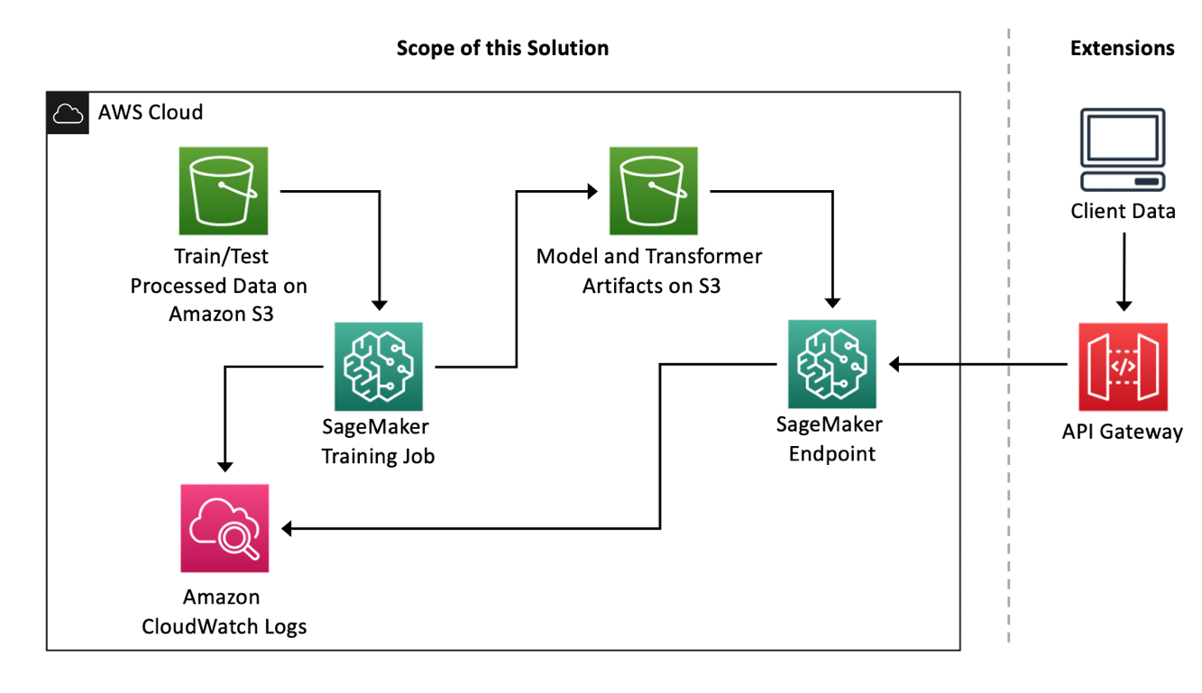
Architecture overview

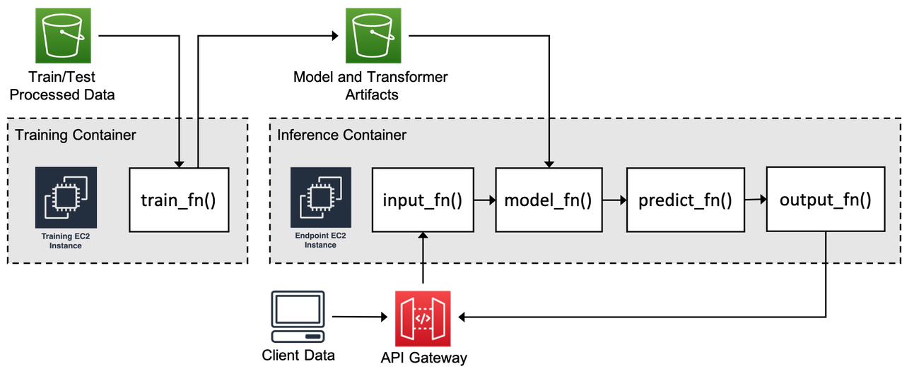
In this solution, we focus on SageMaker components. We use SageMaker training jobs to train the churn prediction model and a SageMaker endpoint to deploy the model. We use Amazon Simple Storage Service (Amazon S3) to store the training data and model artifacts, and Amazon CloudWatch to log training and endpoint outputs. The following figure illustrates the architecture for the solution.

Exploring the data

In this post, we use a mobile operator’s historical records of which customers ended up churning and which continued using the service. The data also includes transcriptions of the latest phone call conversations between the customer and the agent (which could also be the streaming transcription as the call is happening). We can use this historical information to train an ML classifier model, which we can then use to predict the probability of customer churn based on the customer’s profile information and the content of the phone call transcription. We create a SageMaker endpoint to make real-time predictions using the model and provide more insight to customer service agents as they handle customer phone calls.

The dataset we use is synthetically generated and available under the CC BY 4.0 license. The data used to generate the numerical and categorical features is based on the public dataset KDD Cup 2009: Customer relationship prediction. We have generated over 50,000 samples and randomly split the data into 45,000 samples for training and 5,000 samples for testing. In addition, the phone conversation transcripts were synthetically generated using the GPT2 (Generative Pre-trained Transformer 2) algorithm. The data is hosted on Amazon S3.

More details on customer churn classification models using similar data, and also step-by-step instructions on how to build a binary classifier model using similar data, can be found in the blog post Predicting Customer Churn with Amazon Machine Learning. That post is focused more on binary classification using the tabular data. This blog post approaches this problem from a different perspective, and brings in natural language processing (NLP) by processing the context of agent-customer phone conversations.

The following are the attributes (features) of the customer profiles dataset:

  • CustServ Calls – The number of calls placed to customer service
  • State: The US state in which the customer resides, indicated by a two-letter abbreviation; for example, OH or NJ
  • VMail Message – The average number of voice mail messages per month
  • Account Length – The number of days that this account has been active
  • Day Mins, Day Calls, Day Charge – The billed cost for calls placed during the day
  • Eve Mins, Eve Calls, Eve Charge – The billed cost for calls placed during the evening
  • Night Mins, Night Calls, Night Charge – The billed cost for calls placed during nighttime
  • Intl Mins, Intl Calls, Intl Charge – The billed cost for international calls
  • Location – Whether the customer is located in urban, suburban, rural, or other areas
  • State – The state location of the customer
  • Plan – The plan category
  • Limit – Limited or unlimited plan type
  • Text – The synthetic GPT-2 generated transcription of the customer-agent phone conversation
  • Y: Whether the customer left the service (true/false)

The last attribute, Y, is known as the target feature, or the feature we want the ML model to predict. Because the target feature is binary (true/false), the type of modeling is a binary classification model. The model we train later in this post predicts the likelihood of churn as well.

We don’t go over exploratory data analysis in this post. For more details, see Predicting Customer Churn with Amazon Machine Learning and the Customer Churn Prediction with XGBoost sample notebook.

The training script is developed to allow the ML practitioner to pick and choose the features used in training. For example, we don’t use all the features in training. We focus more on the maturity of the customer’s account, number of times the customer has contacted customer service, type of plan they have, and transcription of the latest phone call. You can use additional features in training by including the list in the hyperparameters, as we show in the next section.

The transcription of customer-agent phone call in the text column is synthetic text generated by ML models using the GPT2 algorithm. Its purpose is to show how you can apply this solution to real-world customer service phone conversations. GPT2 is an unsupervised transformer language model developed by OpenAI. It’s a powerful generative NLP model that excels in processing long-range dependencies, and is pre-trained on a diverse corpus of text. For more details on how to generate text using GPT2, see Experimenting with GPT-2 XL machine learning model package on Amazon SageMaker and the Creative Writing using GPT2 Text Generation example notebook.

Train the model

For this post, we use the SageMaker PyTorch Estimator to build a SageMaker estimator using an Amazon-built Docker container that runs functions defined in the supplied entry_point Python script within a SageMaker training job. The training job is started by calling .fit() on this estimator. Later, we deploy the model by calling the .deploy() method on the estimator. Visit Amazon SageMaker Python SDK technical documentation for more details on preparing PyTorch scripts for SageMaker training and using the PyTorch Estimator.

Also, visit Available Deep Learning Containers Images on GitHub to get a list of supported PyTorch versions. At the time of this writing, the latest version available is PyTorch 1.8.1 with Python version 3.6. You can update the framework version to the latest supported version by changing the framework_version parameter in the PyTorch Estimator. You can also use SageMaker utility API image URIs to get the latest list of supported versions.

The hyperparameters dictionary defines which features we want to use for training and also the number of trees in the forest (n-estimators) for the model. You can add any other hyperparameters for the RandomForestClassifier; however, you also need revise your custom training script to receive these parameters in the form of arguments (using the argparse library) and add them to your model. See the following code:

hyperparameters = {
    "n-estimators": 100,
    "numerical-feature-names": "CustServ Calls,Account Length",
    "categorical-feature-names": "plan,limit",
    "textual-feature-names": "text",
    "label-name": "y"
}

estimator = PyTorch(
    framework_version='1.8.1',
    py_version='py3',
    entry_point='entry_point.py',
    source_dir='path/to/source/directory',
    hyperparameters=hyperparameters,
    role=iam_role,
    instance_count=1,
    instance_type='ml.p3.2xlarge',
    output_path='s3://path/to/output/location',
    code_location='s3://path/to/code/location',
    base_job_name=base_job_name,
    sagemaker_session=sagemaker_session,
    train_volume_size=30
)

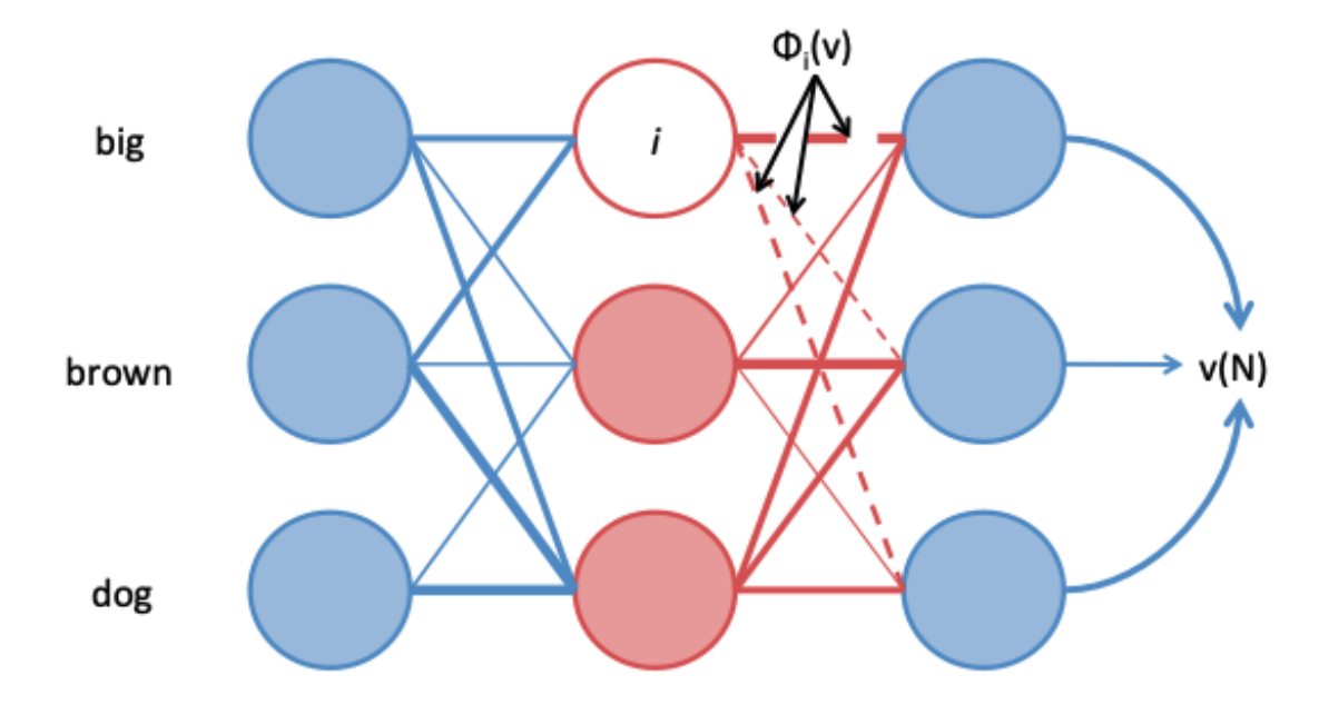
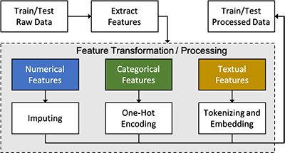
If you launched the SageMaker JumpStart solution in your account, the custom scripts are available in your Studio files. We use the entry_point.py script. This script receives a list of numerical features, categorical features, textual features, and the target label, and trains a SKLearn RandomForestClassifier on the data. However, the key here is processing the features before using them in the classifier, especially the call transcription. The following figure shows this process, which applies imputing to numerical features and replaces missing values with mean, one-hot encoding to categorical features, and embeds transformers to textual features.

The purpose of the script presented in this post is to provide an example of how you can develop your own custom feature transformation pipeline. You can apply other transformations to the data based on your specific use case and the nature of your dataset, and make it as complex or as simple as you want. For example, depending on the nature of your dataset and the results of the exploratory data analysis, you may want to consider normalization, log transformation, or dropping records with null values. For a more complete list of feature transformation techniques, visit SKLearn Dataset Transformations.

The following code snippet shows you how to instantiate these transformers for numerical and categorical features, and how to apply them to your dataset. More details on how these are done in the training script is available in the entry_point.py script that is launched in your files by the JumpStart solution.

from sklearn.impute import SimpleImputer
from sklearn.preprocessing import OneHotEncoder

# Instantiate transformers
numerical_transformer = SimpleImputer(missing_values=np.nan, 
                                        strategy='mean', 
                                        add_indicator=True)
categorical_transformer = OneHotEncoder(handle_unknown="ignore")

# Train transformers on data, and store transformers for future use by predict function
numerical_transformer.fit(numerical_features)
joblib.dump(numerical_transformer, Path(args.model_dir, "numerical_transformer.joblib"))

categorical_transformer.fit(categorical_features)
joblib.dump(categorical_transformer, Path(args.model_dir, "categorical_transformer.joblib"))

# transform the data
numerical_features = numerical_transformer.transform(numerical_features)
categorical_features = categorical_transformer.transform(categorical_features)

Now let’s focus on the textual data. We use Hugging Face sentence transformers, which you can use for sentence embedding generation. They come with pre-trained models that you can use out of the box based on your use case. In this post, we use the bert-base-nli-cls-token model, which is described in Sentence-BERT: Sentence Embeddings using Siamese BERT-Networks.

Recently, SageMaker introduced new Hugging Face Deep Learning Containers (DLCs) that enable you to train, fine-tune, and run inference using Hugging Face models for NLP on SageMaker. In this post, we use the PyTorch container and a custom training script. For this purpose, in our training script, we define a BertEncoder class based on Hugging Face SentenceTransformer and define the pre-trained model as bert-base-nli-cls-token, as shown in the following code. The reason for this is to be able to apply the transformer to the dataset in the same way as the other dataset transformers, with the applying .transform() method. The benefit of using Hugging Face pre-trained models is that you don’t need to do additional training to be able to use the model. However, you can still fine-tune the models with custom data, as described in Fine-tuning a pretrained model.

from sentence_transformers import SentenceTransformer

# Define a class for BertEncoder
class BertEncoder(BaseEstimator, TransformerMixin):
    def __init__(self, model_name='bert-base-nli-cls-token'):
        self.model = SentenceTransformer(model_name)
        self.model.parallel_tokenization = False

    def fit(self, X, y=None):
        return self

    def transform(self, X):
        output = []
        for sample in X:
            encodings = self.model.encode(sample)
            output.append(encodings)
        return output

# Instantiate the class 
textual_transformer = BertEncoder()

# Apply the transformation to textual features
textual_features = textual_transformer.transform(textual_features)

Now that the dataset is processed and ready to be consumed by an ML model, we can train any classifier model to predict if a customer will churn or not. In addition to predicting the class (0/1 or true/false) for customer churn, these models also generate the probability of each class, meaning the probability of a customer churning. This is particularly useful for customer service teams for strategizing the incentives or upgrades they can offer to the customer based on how likely the customer is to cancel the service or subscription. In this post, we use the SKLearn RandomForestClassifier model. You can choose from many hyperparameters for this model and also optimize the hyperparameters for a more accurate model prediction by using strategies like grid search, random search, and Bayesian search. SageMaker automatic hyperparameter tuning can be a powerful tool for this purpose.

Training the model in entry_point.py is handled by the train_fn() function in the custom script. This function is called when the .fit() method is applied to the estimator. This function also stores the trained model and trained data transformers on Amazon S3. These files are used later by model_fn() to load the model for inference purposes.

train_fn() also includes evaluation of the trained model, and provides accuracy scores for the model for both train and test datasets. This helps you better evaluate model performance. Because this is a classification problem, we recommend including other metrics in your evaluation script, for example F1 score, ROC AUC score, and recall score, the same way we added accuracy scores. These are printed as the training progresses. Because we’re using synthetic data for training the model in this example notebook, especially for the agent-customer call transcription, we’re not expecting to see high-performing models with regards to classification metrics, and therefore we’re not focusing on these metrics in this example. However, when you use your own data, you should consider how each classification metric could impact the applicability of the model to your use case. Training this model on 45,000 samples on an ml.p3.2xlarge instance takes about 30 minutes.

estimator.fit({
    'train': 's3://path/to/your/train.jsonl')),
    'test': 's3://path/to/your/test.jsonl'))
})

When you’re comfortable with the performance of your model, you can move to the next step, which is deploying your model for real-time inference.

Deploy the model

When the training is complete, you can deploy the model as a SageMaker hosted endpoint for real-time inference, or use the model for offline batch inference, using SageMaker batch transform. The task of performing inference (either real time or batch) is handled by four main functions in the custom script:

  • input_fn() processes the input data
  • model_fn() loads the trained model artifacts from Amazon S3
  • predict_fn() makes predictions
  • output_fn() prepares the model output

The following diagram illustrates this process.

The following script is a snippet of the entry_point.py script, and shows how the four functions work together to perform inference:

# Model function to load the trained model and trained transformers from S3
def model_fn(model_dir):
    print('loading feature_names')
    numerical_feature_names, categorical_feature_names, textual_feature_names = load_feature_names(Path(model_dir, "feature_names.json"))
    print('loading numerical_transformer')
    numerical_transformer = joblib.load(Path(model_dir, "numerical_transformer.joblib"))
    print('loading categorical_transformer')
    categorical_transformer = joblib.load(Path(model_dir, "categorical_transformer.joblib"))
    print('loading textual_transformer')
    textual_transformer = BertEncoder()
    classifier = joblib.load(Path(model_dir, "classifier.joblib"))
    model_assets = {
        'numerical_feature_names': numerical_feature_names,
        'numerical_transformer': numerical_transformer,
        'categorical_feature_names': categorical_feature_names,
        'categorical_transformer': categorical_transformer,
        'textual_feature_names': textual_feature_names,
        'textual_transformer': textual_transformer,
        'classifier': classifier
    }
    return model_assets


# Input Preparation Function to receive the request body and ensure proper format
def input_fn(request_body_str, request_content_type):
    assert (
        request_content_type == "application/json"
    ), "content_type must be 'application/json'"
    request_body = json.loads(request_body_str)
    return request_body


# Predict function to make inference
def predict_fn(request, model_assets):
    print('making batch')
    request = [request]
    print('extracting features')
    numerical_features, categorical_features, textual_features = extract_features(
        request,
        model_assets['numerical_feature_names'],
        model_assets['categorical_feature_names'],
        model_assets['textual_feature_names']
    )
    
    print('transforming numerical_features')
    numerical_features = model_assets['numerical_transformer'].transform(numerical_features)
    print('transforming categorical_features')
    categorical_features = model_assets['categorical_transformer'].transform(categorical_features)
    print('transforming textual_features')
    textual_features = model_assets['textual_transformer'].transform(textual_features)
    
    # Concatenate Features
    print('concatenating features')
    categorical_features = categorical_features.toarray()
    textual_features = np.array(textual_features)
    textual_features = textual_features.reshape(textual_features.shape[0], -1)
    features = np.concatenate([
        numerical_features,
        categorical_features,
        textual_features
    ], axis=1)
    
    print('predicting using model')
    prediction = model_assets['classifier'].predict_proba(features)
    probability = prediction[0][1].tolist()
    output = {
        'probability': probability
    }
    return output

# Output function to prepare the output
def output_fn(prediction, response_content_type):
    assert (
        response_content_type == "application/json"
    ), "accept must be 'application/json'"
    response_body_str = json.dumps(prediction)
    return response_body_str

To deploy the model, when the training is complete, we use the .deploy() method on the estimator and define the number and type of instances we want to attach to the endpoint, and SageMaker manages the infrastructure on your behalf. When calling the endpoint from the notebook, we use a SageMaker SDK predictor. The predictor sends data to an endpoint (as part of a request), and interprets the response. See the following code:

# Deploy the predictor
predictor = estimator.deploy(
    endpoint_name=endpoint_name,
    instance_type='ml.p3.2xlarge',
    initial_instance_count=1
)

predictor.serializer = JSONSerializer()
predictor.deserializer = JSONDeserializer()

This deploys the model as an endpoint predictor. After deployment is complete, we can use that to make predictions on sample data. Let’s determine the probability of churn for a hypothetical customer:

data = {
    "CustServ Calls": 10.0,
    "Account Length": 66,
    "plan": "B",
    "limit": "limited",
    'text': "Well, I've been dealing with TelCom for three months now and I am quite happy with your service"}

response = predictor.predict(data=data)

print("{:.2%} probability of churn".format(response['probability']))

In this case, the probability of churn is about 31%. For the same customer, we change the transcript to “I have been using your service for 6 months and I am disappointed in your customer service.” The probability of churn increases to over 46%. This demonstrates that a change in the customer’s sentiment affects the probability of churn.

Clean up

To clean up the resources and stop incurring charges in your account, you can delete the endpoint:

predictor.delete_endpoint()

Extensions

As we explained earlier, you can use additional features in training and also incorporate more feature transformers in the feature engineering pipeline, which can help improve model performance.

In addition, now that you have a working endpoint that is performing real-time inference, you can use it for your applications or website. However, your SageMaker endpoint is still not public facing, so you need to build an API Gateway to allow external traffic to your SageMaker endpoint. Amazon API Gateway is a fully managed service that makes it easy for developers to create, publish, maintain, monitor, and secure APIs at any scale. You can use API Gateway to present an external-facing, single point of entry for SageMaker endpoints, and provide security, throttling, authentication, firewall as provided by AWS WAF, and more. With API Gateway mapping templates, you can invoke your SageMaker endpoint with a REST API request and receive an API response back without needing any intermediate AWS Lambda functions, thereby improving the performance and cost-effectiveness of your applications.

To create an API Gateway and use it to perform real-time inference with your SageMaker endpoint (see the following architecture), you can follow the instructions outlined in Creating a machine learning-powered REST API with Amazon API Gateway mapping templates and Amazon SageMaker.

In addition, you can use Amazon Transcribe to generate transcriptions of recorded customer-agent conversations and use them for training purposes, and also use Amazon Transcribe streaming to send the conversation audio stream and receive a stream of text in real time. You can use this text stream to add a real-time speech-to-text capability to your applications and also send that text to the endpoint and provide customer churn insights to your customer service agents in real time.

Conclusions

In this post, we explained an end-to-end solution for creating a customer churn prediction model based on customer profiles and customer-agent call transcriptions. The solution included training a PyTorch model with a custom script and creating an endpoint for real-time model hosting. We also explained how you can create a public-facing API Gateway that can be securely used in your mobile applications or website. In addition, we explained how you can use Amazon Transcribe for batch or real-time transcription of customer-agent conversations, which you can use for training of your model or real-time inference.

For more SageMaker examples, visit the Amazon SageMaker Examples GitHub repo. For more PyTorch BYO script examples, visit the following GitHub repository. For more SageMaker Python examples for MXNet, TensorFlow, and PyTorch, visit the Amazon SageMaker Pre-Built Framework Containers and the Python SDK GitHub repo. Additional information about SageMaker is available in the technical documentation.


About the Author

Nick Minaie is an Sr AI/ML Specialist Solutions Architect with AWS, helping customers on their journey to well-architected machine learning solutions at scale. In his spare time, Nick enjoys family time, abstract painting, and exploring nature.


Ehsan M. Kermani is a Machine Learning Engineer in the AWS ML Automation Services group. He helps customers through their MLOps journey by providing his expertise in Software Engineering best practices to solve customers’ end-to-end Machine Learning tasks from infrastructure to deployment.


Dr. Li Zhang is a Principal Product Manager-Technical for Amazon SageMaker JumpStart and Amazon SageMaker built-in algorithms, a service that helps data scientists and machine learning practitioners get started with training and deploying their models, and uses reinforcement learning with Amazon SageMaker. His past work as a principal research staff member and master inventor at IBM Research has won the test of time paper award at IEEE INFOCOM.

Read More

Get started with the Amazon Kendra Amazon WorkDocs connector

Amazon Kendra is an intelligent search service powered by machine learning (ML). Amazon Kendra reimagines enterprise search for your websites and applications so your employees and customers can easily find the content they’re looking for, even when it’s scattered across multiple locations and content repositories within your organization.

With Amazon Kendra, you can search through troves of unstructured data and discover the right answers to your questions, when you need them. Amazon Kendra is a fully managed service, so there are no servers to provision, and no ML models to build, train, or deploy.

Amazon WorkDocs is a fully managed and secure content creation, storage, and collaboration service. With Amazon WorkDocs, you can easily create, edit, and share content. Moreover, because it’s stored centrally on AWS, you can access it from anywhere on any device.

In this post, we show how Amazon Kendra allows your users to search documents stored in Amazon WorkDocs.

Use case

For this post, we created a specific folder in Amazon WorkDocs containing a set of PDFs and Microsoft Word documents that we want to search content on. The Amazon WorkDocs connector also allows you to ingest comments for those documents.

The following screenshot shows the contents of a fictional WorkDocs folder called WorkdocsBlogpostDataset.

Create an Amazon WorkDocs connector

To create an Amazon WorkDocs connector, complete the following steps:

  1. On the Amazon Kendra console, choose Data sources.
  2. Choose Add data source.
  3. Under WorkDocs, choose Add connector.
  4. For Data source name, enter a name for your data source.
  5. Enter an optional description.
  6. Choose Next.
  7. In the Source section, choose the organization ID for your Amazon WorkDocs site.
  8. Create a new AWS Identity and Access Management (IAM) role for the data source.
  9. For Sync scope, select Crawl document comments and Use change logs.

For this post, we want Amazon Kendra to ingest the documents in the WorkdocsBlogpostDataset folder.

  1. In the Additional configuration section, enter WorkdocsBlogpostDataset as a path on the Include patterns tab.
  2. Choose Add.
  3. For Sync run schedule¸ choose Run on demand.
  4. Choose Next.
  5. In the WorkDocs field mapping section, use the default field mapping.
  6. Choose Next.
  7. Review the settings and choose Create.
  8. When the creation process is complete, choose Sync.

When the sync process complete, you can see how many documents were ingested.

Now your documents are ready be searched by Amazon Kendra.

  1. In the navigation pane, choose Search console.

You can now submit some test queries, as shown in the following screenshots.

Also, with the Amazon WorkDocs connector, you can ingest feedback (comments) on your documents. For example, the following screenshot shows that this document has feedback.

The following screenshot shows what the feedback search experience looks like.

Conclusion

In this post, you created a data source and ingested your Amazon WorkDocs documents into your Amazon Kendra index. As a next step, you can try some more queries and see what kind of results you obtain. You can also dive deep into Amazon Kendra with the Amazon Kendra Essentials workshop or try the multilingual chatbot experience.


About the Author

Juan Bustos is an AI Services Specialist Solutions Architect at Amazon Web Services, based in Dallas, TX. Outside of work, he loves spending time writing and playing music as well as trying random restaurants with his family.


Vijai Gandikota is a Senior Product Manager at Amazon Web Services for Amazon Kendra.

Read More

Investing in academic research to improve our privacy technology: Our approach and recent RFP winners

One of our goals over the next decade is to build stronger privacy protections for everyone who uses our apps and services. Our latest research award opportunity in privacy-enhancing technology and the recently launched request for proposals on Building Tools to Enhance Transparency in Fairness and Privacy are the next of many steps toward that goal, and a continuation of several years of investments in the privacy research space.

Our approach to academic research and investments

Through a variety of programs, partnerships, and collaborations, Facebook researchers work with the global academic community on topics that align with our mission to give people the power to build community and bring the world closer together. “We are sponsoring labs and conferences, partnering with academics on short- and long-term projects, and supporting PhD students through our Fellowship program,” says Sharon Ayalde, Research Program Manager, Facebook Academic Engagements. “We also provide research award opportunities through open requests for proposals.”

Requests for proposals (RFPs) in particular help us strengthen our ties to academia and foster community. Through RFPs, we are able to discover activities and key players in academia that are aligned with our research challenges. Research funds are generally awarded as unrestricted gifts to accredited universities to help finance winning proposals. In general, there are 15 to 20 RFP opportunities each year across a variety of research topics, such as privacy, networking, data science, probability, machine learning, and UX.

Investing in these research projects helps accelerate the field for everyone and allows us to apply the most cutting-edge technologies to our apps and services. In the privacy research space, we’ve steadily increased opportunities for academic collaboration, and research project funding continues to be available. Last year, we granted research awards in key topics such as privacy-preserving technologies and cryptography, user experiences in privacy, and privacy in AR/VR and smart device products. These opportunities alone attracted more than 300 applications, with over $2 million in total funding.

The 2020 People’s Expectations and Experiences with Digital Privacy RFP, in particular, received 147 proposals from 34 countries and 120 universities. The five winning proposals represented 14 universities, including Cornell University, Carnegie Mellon University, the Hebrew University of Jerusalem, India Institute of Technology, Brigham Young University, Northwestern University, and Hamad Bin Khalifa University.

What’s next

In 2021 and beyond, we will continue our investment in research and innovation to help us develop new ways to build products and process data with privacy in mind. We’ll also continue to work with policymakers, privacy experts, global organizations and developers on building solutions to ensure that people feel safe and comfortable using our products.

“Our world and the role of technology in our lives and society is evolving faster than ever before,” says Scott Renfro, Facebook Software Engineer. “It’s critical that we work hard to put privacy, safety, and security first and work with people at the forefront of emerging technologies and scientific understanding to find better solutions. This is why we want to collaborate with academia and support the important work they do by launching another research award opportunity.”

As part of our continued investment, we are pleased to announce the winners and finalists of the 2021 Privacy-Enhancing Technologies RFP, which sought proposals from academics conducting research in applied cryptography, data policies and compliance, differential privacy, and privacy in AI. The research award opportunity attracted 159 proposals from 102 universities. Thank you to everyone who took the time to submit a proposal, and congratulations to the winners.

Research award recipients

Principal investigators are listed first unless otherwise noted.

Bridging secure computation and differential privacy
Jonathan Katz (University of Maryland College Park)

Cryptographic enforcement of end-to-end data privacy
Anwar Hithnawi (ETH Zurich)

Implementing a flexible framework for privacy accounting
Salil Vadhan (Harvard University)

InferViz: Weighted inference and visualization of insecure code paths
Musard Balliu (KTH Royal Institute of Technology), Marco Guarnieri (IMDEA Software Institute)

Practical differential privacy: Using past and present to inform future
Aleksandra Korolova, Brendan Avent (University of Southern California)

Privacy-preserving machine learning via ADMM
Yupeng Zhang (Texas A&M University)

Private authentication with complex assertions and abuse prevention
Ian Miers (University of Maryland College Park)

Safeguarding user data against cross-library data harvesting
Luyi Xing, Xiaojing Liao (Indiana University Bloomington)

SEBRA: SEcuring BRowser Extensions by Information Flow Analysis
Andrei Sabelfeld (Chalmers University of Technology)

Towards privacy-preserving and fair ad targeting with federated learning
Golnoosh Farnadi (HEC Montreal and MILA), Martine De Cock (University of Washington Tacoma)

Finalists

A methodological approach to privacy-preserving data analysis pipelines
Patrick Thomas Eugster, Savvas Savvides (Università della Svizzera italiana)

A toolkit for locally private statistical inference
Clement Canonne, Vincent Gramoli (University of Sydney)

Advancing differential privacy accounting
Yu-Xiang Wang (University of California Santa Barbara)

An informed consent management engine to control the privacy of IoT devices
John Grundy, Mohan Chhetri, Zubir Baig, Chehara Pathmabandu (Monash University)

Beyond cookies: Private personalization for the tracker-free web
Henry Corrigan-Gibbs (Massachusetts Institute of Technology)

Challenges in E2E encryption
Yevgeniy Dodis (New York University)

Consent flows tracking for OAuth2.0 standard protocol
Alex Pentland, Thomas Hardjono (Massachusetts Institute of Technology)

Deletion compliance in data systems
Manos Athanassoulis (Boston University)

Differentially private analyses of textual data, such as Facebook posts
Gary King (Harvard University)

Differentially private collection of key-value pairs using multi-party computation
Florian Kerschbaum (University of Waterloo)

Differentially private analysis of streaming and graph data
Jerome Le Ny (Polytechnique Montreal)

Differentially private multi-task learning
Virginia Smith, Steven Wu (Carnegie Mellon University)

DragonFLy: Private, efficient, and accurate federated learning
Adam O’Neill, Amir Houmansadr (University of Massachusetts Amherst)

Efficient sparse vector aggregation for private federated learning
Giulia Fanti, Elaine Shi (Carnegie Mellon University)

End-to-end privacy compliance in distributed web services
Malte Schwarzkopf (Brown University)

Fast identity online with attributes and global revocation (sFIDO)
Lucjan Hanzlik (CISPA Helmholtz Center for Information Security)

InferViz: Weighted inference and visualization of insecure code paths
Musard Balliu (KTH Royal Institute of Technology), Marco Guarnieri (IMDEA Software Institute)

Practical private information retrieval with privacy-enhancing applications
Ling Ren (University of Illinois Urbana-Champaign)

Privacy-preserving machine learning through label differential privacy
Prateek Mittal, Amir Houmansadr (Princeton University)

Privacy in sketches for big data analytics
Pedro Reviriego-Vasallo (University Carlos III de Madrid)

Privacy of data set properties in machine learning
Olga Ohrimenko (University of Melbourne)

Searching for accurate and efficient private models
Reza Shokri (National University of Singapore)

Symmetric homomorphic encryption for fast privacy-preserving data analysis
Patrick Thomas Eugster, Savvas Savvides (Università della Svizzera italiana)

Scalable and secure protocols for data linking and analytics
Xiao Wang (Northwestern University)

The post Investing in academic research to improve our privacy technology: Our approach and recent RFP winners appeared first on Facebook Research.

Read More

Setting the Virtual Stage: ‘Deathtrap Dungeon’ Gets Interactive Thanks to NVIDIA RTX

Deathtrap Dungeon: The Golden Room is a gripping choose-your-own-adventure story, but it’s no page-turner.

Based on the best-selling book of the same name, it’s an interactive film in which viewers become the player on their quest to find The Golden Room while facing down dungeon masters and avoiding traps.

NVIDIA RTX technology powers the real-time graphics and virtual sets behind this latest adaptation, which showcases the future of interactive storytelling on a virtual production stage.

On-Set Facilities (OSF) provided the technology for the virtual production. Using its own low-latency computing platform, the GODBOX powered by NVIDIA RTX, OSF enhanced virtual production workflows and delivered real-time compositing and previsualization for the interactive experience.

Bringing Virtual Sets to Life with NVIDIA RTX

When it comes to bringing VFX on set, OSF faced a common challenge — finding computers that could be configured for their creative teams and production needs. So they created their own on-set computer platform, GODBOX Workstations and Servers. It’s a synchronized real-time virtual production platform for low-latency, frame-accurate, virtual production applications and workflows.

From LED and in-camera VFX to mixed reality and motion capture, the GODBOX provides all the tools, features and solutions needed to set up and run a virtual production from any set.

All images courtesy of On-Set Facilities.

For Deathtrap Dungeon, OSF laid the foundations during preproduction and previsualization. The team used virtual sets and real locations, and combined that with real-time visual effects to bring sets to life. Digitally creating the previsual assets allowed the team to specify the size of stages, amounts of props and how many physical sets were needed.

“The objective was to previsualize the final VFX on the set, so that the directors, actors and crew could all see the virtual world,” said Asa Bailey, director of virtual production at OSF. “The GODBOX delivers in-camera VFX and real-time compositing pipelines powered by NVIDIA RTX. The platform was specifically designed to work with all kinds of virtual productions.”

Throughout the preproduction and the film shoot, OSF used Unreal Engine to conduct virtual scouting sessions using the GODBOX cloud production VPN. Using the secure cloud platform, OSF tested the virtual sets and worked with the production to set lighting and camera movements, all before going on set.

With the RTX-powered GODBOX, OSF also delivered real-time compositing so the cast and crew can see their performance with the virtual set and characters.  The team combined green screen live action with virtual sets and VFX elements in Unreal Engine. Then they’d take the real-time composition and feed it through to large screens and projectors on set.

OSF’s GODBOX stays updated with the latest NVIDIA drivers, as well as recently released optimizations. This helps increase the stability of the machine, which becomes crucial when the cameras are rolling.

Learn more about On-Set Facilities, GODBOX low-latency computing and virtual production. And see other NVIDIA solutions in media and entertainment.

The post Setting the Virtual Stage: ‘Deathtrap Dungeon’ Gets Interactive Thanks to NVIDIA RTX appeared first on The Official NVIDIA Blog.

Read More