Posts in category: Amazon AWS

This is a guest post co-authored by Nafi Ahmet Turgut, Mutlu Polatcan, Pınar Baki, Mehmet İkbal Özmen, Hasan Burak Yel, and Hamza Akyıldız from Getir.

Getir is the pioneer of ultrafast grocery delivery. The tech company has revolutionized last-mile delivery with its “groceries in minutes” delivery proposition. Getir was founded in 2015 and operates in Turkey, the UK, the Netherlands, Germany, France, Spain, Italy, Portugal, and the United States. Today, Getir is a conglomerate incorporating nine verticals under the same brand.

Predicting future demand is one of the most important insights for Getir and one of the biggest challenges we face. Getir relies heavily on accurate demand forecasts at a SKU level when making business decisions in a wide range of areas, including marketing, production, inventory, and finance. Accurate forecasts are necessary for supporting inventory holding and replenishment decisions. Having a clear and reliable picture of predicted demand for the next day or week allows us to adjust our strategy and increase our ability to meet sales and revenue goals.

Getir used Amazon Forecast, a fully managed service that uses machine learning (ML) algorithms to deliver highly accurate time series forecasts, to increase revenue by four percent and reduce waste cost by 50 percent. In this post, we describe how we used Forecast to achieve these benefits. We outline how we built an automated demand forecasting pipeline using Forecast and orchestrated by AWS Step Functions to predict daily demand for SKUs. This solution led to highly accurate forecasting for over 10,000 SKUs across all countries where we operate, and contributed significantly to our ability to develop high scalable internal supply chain processes.

Forecast automates much of the time-series forecasting process, enabling you to focus on preparing your datasets and interpreting your predictions.

Step Functions is a fully managed service that makes it easier to coordinate the components of distributed applications and microservices using visual workflows. Building applications from individual components that each perform a discrete function helps you scale more easily and change applications more quickly. Step Functions automatically triggers and tracks each step and retries when there are errors, so your application executes in order and as expected.

Solution overview

Six people from Getir’s data science team and infrastructure team worked together on this project. The project was completed in 3 months and deployed to production after 2 months of testing.

The following diagram shows the solution’s architecture.

The model pipeline is executed separately for each country. The architecture includes four Airflow cron jobs running on a defined schedule. The pipeline starts with feature creation which first creates the features and loads them to Amazon Redshift. Next, a feature processing job prepares daily features stored in Amazon Redshift and unloads the time series data to Amazon Simple Storage Service (Amazon S3). A second Airflow job is responsible for triggering the Forecast pipeline via Amazon EventBridge. The pipeline consists of Amazon Lambda functions, which create predictors and forecasts based on parameters stored in Amazon S3. Forecast reads data from Amazon S3, trains the model with hyperparameter optimization (HPO) to optimize model performance, and produces future predictions for product sales. Then the Step Functions “WaitInProgress” pipeline is triggered for each country, which enables parallel execution of a pipeline for each country.

Algorithm Selection

Amazon Forecast has six built-in algorithms (ARIMA, ETS, NPTS, Prophet, DeepAR+, CNN-QR), which are clustered into two groups: statististical and deep/neural network. Among those algorithms, deep/neural networks are more suitable for e-commerce forecasting problems as they accept item metadata features, forward-looking features for campaign and marketing activities, and – most importantly – related time series features. Deep/neural network algorithms also perform very well on sparse data set and in cold-start (new item introduction) scenarios.

Overall, in our experimentations, we observed that deep/neural network models performed significantly better than the statistical models. We therefore focused our deep-dive testing on DeepAR+ and CNN-QR

One of the most important benefits of Amazon Forecast is scalability and accurate results for many product and country combinations. In our testing both DeepAR+ and CNN-QR algorithms brought success in capturing trends and seasonality, allowing us to obtain efficient results in products whose demand changes very frequently.

Deep AutoRegressive Plus (DeepAR+) is a supervised univariate forecasting algorithm based on recurrent neural networks (RNNs) created by Amazon Research. Its main advantages are that it is easily scalable, able to incorporate relevant co-variates into the data (such as related data and metadata), and able to forecast cold-start items. Instead of fitting separate models for each time series, it creates a global model from related time series to handle widely-varying scales through rescaling and velocity-based sampling. The RNN architecture incorporates binomial likelihood to produce probabilistic forecasting and is advocated to outperform traditional single-item forecasting methods (like Prophet) by the authors of DeepAR: Probabilistic Forecasting with Autoregressive Recurrent Networks.

We ultimately selected the Amazon CNN-QR (Convolutional Neural Network – Quantile Regression) algorithm for our forecasting due to its high performance in the backtest process. CNN-QR is a proprietary ML algorithm developed by Amazon for forecasting scalar (one-dimensional) time series using causal Convolutional Neural Networks (CNNs).

As previously mentioned, CNN-QR can employ related time series and metadata about the items being forecasted. Metadata must include an entry for all unique items in the target time series, which in our case are the products whose demand we are forecasting. To improve accuracy, we used category and subcategory metadata, which helped the model understand the relationship between certain products, including complementary and substitutes. For example, for beverages, we provide an additional flag for snacks since the two categories are complementary to each other.

One significant advantage of CNN-QR is its ability to forecast without future related time series, which is important when you can’t provide related features for the forecast window. This capability, along with its forecast accuracy, meant that CNN-QR produced the best results with our data and use case.

Forecast Output

Forecasts created through the system are written to separate S3 buckets after they are received on a country basis. Then, forecasts are written to Amazon Redshift based on SKU and country with daily jobs. We then carry out daily product stock planning based on our forecasts.

On an ongoing basis, we calculate mean absolute percentage error (MAPE) ratios with product-based data, and optimize model and feature ingestion processes.

Conclusion

In this post, we walked through an automated demand forecasting pipeline we built using Amazon Forecast and AWS Step Functions.

With Amazon Forecast we improved our country-specific MAPE by 10 percent. This has driven a four percent revenue increase, and decreased our waste costs by 50 percent. In addition, we achieved an 80 percent improvement in our training times in daily forecasts in terms of scalability. We are able to forecast over 10,000 SKUs daily in all the countries we serve.

For more information about how to get started building your own pipelines with Forecast, see Amazon Forecast resources. You can also visit AWS Step Functions to get more information about how to build automated processes and orchestrate and create ML pipelines. Happy forecasting, and start improving your business today!

About the Authors

Nafi Ahmet Turgut finished his Master’s Degree in Electrical & Electronics Engineering and worked as graduate research scientist. His focus was building machine learning algorithms to simulate nervous network anomalies. He joined Getir in 2019 and currently works as a Senior Data Science & Analytics Manager. His team is responsible for designing, implementing, and maintaining end-to-end machine learning algorithms and data-driven solutions for Getir.

Mutlu Polatcan is a Staff Data Engineer at Getir, specializing in designing and building cloud-native data platforms. He loves combining open-source projects with cloud services.

Pınar Baki received her Master’s Degree from the Computer Engineering Department at Boğaziçi University. She worked as a data scientist at Arcelik, focusing on spare-part recommendation models and age, gender, emotion analysis from speech data. She then joined Getir in 2022 as a Senior Data Scientist working on forecasting and search engine projects.

Mehmet İkbal Özmen received his Master’s Degree in Economics and worked as Graduate Research Assistant. His research area was mainly economic time series models, Markov simulations, and recession forecasting. He then joined Getir in 2019 and currently works as Data Science & Analytics Manager. His team is responsible for optimization and forecast algorithms to solve the complex problems experienced by the operation and supply chain businesses.

Hasan Burak Yel received his Bachelor’s Degree in Electrical & Electronics Engineering at Boğaziçi University. He worked at Turkcell, mainly focused on time series forecasting, data visualization, and network automation. He joined Getir in 2021 and currently works as a Lead Data Scientist with the responsibility of Search & Recommendation Engine and Customer Behavior Models.

Hamza Akyıldız received his Bachelor’s Degree of Mathematics and Computer Engineering at Boğaziçi University. He focuses on optimizing machine learning algorithms with their mathematical background. He joined Getir in 2021, and has been working as a Data Scientist. He has worked on Personalization and Supply Chain related projects.

Esra Kayabalı is a Senior Solutions Architect at AWS, specializing in the analytics domain including data warehousing, data lakes, big data analytics, batch and real-time data streaming and data integration. She has 12 years of software development and architecture experience. She is passionate about learning and teaching cloud technologies.

Read More

Amazon Textract is a machine learning (ML) service that automatically extracts text, handwriting, and data from any document or image. To make it simpler to evaluate the capabilities of Amazon Textract, we have launched a new Bulk Document Uploader feature on the Amazon Textract console that enables you to quickly process your own set of documents without writing any code.

In this post, we walk through when and how to use the Amazon Textract Bulk Document Uploader to evaluate how Amazon Textract performs on your documents.

Overview of solution

The Bulk Document Uploader should be used for quick evaluation of Amazon Textract for predetermined use cases. By uploading multiple documents simultaneously through an intuitive UI, you can easily gauge how well Amazon Textract performs on your documents.

You can upload and process up to 150 documents at once. Unlike the existing Amazon Textract console demos, which impose artificial limits on the number of documents, document size, and maximum allowed number of pages, the Bulk Document Uploader supports processing up to 150 documents per request and has the same document size and page limits as the Amazon Textract APIs. This makes it more efficient for you to evaluate a larger set of documents.

The Bulk Document Uploader outputs a standard Amazon Textract JSON response and CSV file. The results are provided in JSON format for easy programmatic analysis. Additionally, a human-readable CSV file with confidence scores is provided for simple comparison and evaluation of the extracted information.

When using this feature, keep in mind the following:

• The Bulk Document Uploader processes documents via asynchronous operations. You can track the status of the processing on the Amazon Textract console. Only DetectDocumentText (OCR), AnalyzeDocument (Tables, Queries, Forms, and Signatures), and AnalyzeExpense APIs are currently supported.
• The Bulk Document Uploader provides JSON results of the API operations and formatted CSV reports. You may need to rely on external tools for visualization of the data, such as displaying bounding box highlights on the document using the JSON results.
• Using this feature to process documents incurs the same charges as regular Amazon Textract usage (depending on which feature is used), and is subject to the TPS (transactions per second) limits for APIs that are set for the account and Region. For more information on pricing, refer to Amazon Textract pricing. To learn more about Amazon Textract limits, refer to Quotas in Amazon Textract.
• Accepted file formats for bulk uploader are JPEG, PNG, TIF, and PDF. JPEG 2000-encoded images within PDFs are also supported. JPEG and PNG files have a 10 MB size limit, whereas PDF and TIF files have a 500 MB size limit. Multi-page PDF and TIF files have a 3,000 page limit.

Use the Bulk Document Uploader

The Bulk Document Uploader is intended to help you quickly evaluate how Amazon Textract performs on a set of your own documents, without needing to write any code. You can use the Bulk Document Uploader to process as many as 150 documents instead of uploading and processing documents individually. You can bulk upload documents directly from your computer or import documents from an existing Amazon Simple Storage Service (Amazon S3) bucket.

The Bulk Document Uploader provides results that you can download later for offline review. Each downloadable ZIP file contains the Amazon Textract API response in JSON file format and a human-readable CSV file of the output containing the extracted data and confidence scores. The output results are available for download for 7 days after processing. After 14 days, documents are cleared from the Submitted documents section. To use the Bulk Document Uploader, complete the following steps:

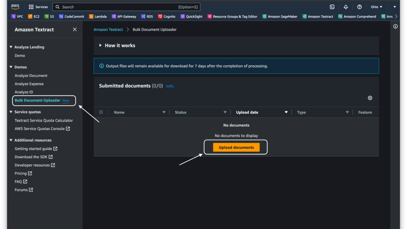
1. On the Amazon Textract console, under Demos in the navigation pane, choose Bulk Document Uploader.
2. Choose Upload documents.
   
3. Specify the source of your documents.

You have two options to upload documents:

• Import documents from S3 bucket – If you’re using an S3 bucket for your documents, provide the bucket URL and (optionally) the prefix where your documents reside, in s3://your-bucket/prefix/ format. Alternatively, choose Browse S3 to browse and select the desired location of your documents. If the Amazon S3 location you specified contains more than 150 documents, then only the first 150 documents will be sent to Amazon Textract for processing.
  
• Upload documents from your computer – If you’re uploading documents from your computer, you can upload up to 50 documents at a time by choosing Upload Documents. To upload additional documents (up to the maximum of 150), choose Add documents after your initial documents are uploaded.
  

In this case, your documents are first uploaded to an S3 bucket in your account that is created on your behalf, therefore it’s important to ensure that you have permissions to access and upload documents to Amazon S3. This is a one-time action, and the same bucket will be used for all subsequent uploads from your computer. If you want to upload and process the same set of documents, you can use the path to this S3 bucket using the Import documents from S3 bucket option. The S3 bucket created on your behalf will be visible after the bucket gets created.

4. Next, specify the Amazon Textract feature you want to use to process your documents.

You may select only one feature at a time to process your documents. If you need to evaluate additional features, you must create a separate request by selecting the desired feature and uploading the documents again. If the AnalyzeDocument – Queries feature is selected, you need to provide the queries you want to test against your documents. You can specify up to 30 queries at a time. If the uploaded documents contain multi-page (PDF or TIF) files, queries are only applied to the first page of each document. Refer to Best Practices for Queries to learn about how to construct queries.

5. Choose Start processing to submit the documents to Amazon Textract for processing.

You can track the document status and download the output results of processed documents in the Submitted documents section. This section updates periodically, and you can manually refresh it to see if the processing is complete. Each document is processed individually, so you can either select the document with Ready to download status or wait for all documents to complete processing to download the results. The output of the processed documents will remain available for up to 7 days for download, after which they will expire. Expired documents will be cleared from the Submitted documents section after 7 additional days (14 days from the processed date). We suggest downloading and preserving the outputs within the 7-day period.

Conclusion

In this post, we announced the new Amazon Textract Bulk Document Uploader feature, which allows you to quickly process a large number of documents for evaluation purposes. You can use this feature to evaluate Amazon Textract for a predetermined use case with your documents. To learn more about how you can use Amazon Textract in your intelligent document processing workload, visit Amazon Textract features and Getting started with Amazon Textract.

About the Authors

Shashwat Sapre is a Senior Technical Product Manager with the Amazon Textract team. He is focused on building machine learning-based services for AWS customers. In his spare time, he likes reading about new technologies, traveling and exploring different cuisines.

Anjan Biswas is a Senior AI Services Solutions Architect with a focus on AI/ML and Data Analytics. Anjan is part of the world-wide AI services team and works with customers to help them understand and develop solutions to business problems with AI and ML. Anjan has over 14 years of experience working with global supply chain, manufacturing, and retail organizations, and is actively helping customers get started and scale on AWS AI services.

Read More

Amazon SageMaker comes with two options to spin up fully managed notebooks for exploring data and building machine learning (ML) models. The first option is fast start, collaborative notebooks accessible within Amazon SageMaker Studio—a fully integrated development environment (IDE) for machine learning. You can quickly launch notebooks in Studio, easily dial up or down the underlying compute resources without interrupting your work, and even share your notebook as a link in few clicks. In addition to creating notebooks, you can perform all the ML development steps to build, train, debug, track, deploy, and monitor your models in a single pane of glass in Studio. The second option is Amazon SageMaker notebook instances—a single, fully managed ML compute instance running notebooks in the cloud, offering you more control on your notebook configurations.

Today, we are excited to announce the availability of Amazon CodeWhisperer and Amazon CodeGuru Security extensions in SageMaker notebooks. These AI-powered extensions help accelerate ML development by offering code suggestions as you type, and ensure that your code is secure and follows AWS best practices.

In this post, we show how you can get started with Amazon CodeGuru Security and CodeWhisperer in Studio and SageMaker notebook instances.

Solution overview

The CodeWhisperer extension is an AI coding companion that provides developers with real-time code suggestions in notebooks. Individual developers can use CodeWhisperer for free in Studio and SageMaker notebook instances. The coding companion generates real-time single-line or full function code suggestions. It understands semantics and context in your code and can recommend suggestions built on AWS and development best practices, improving developer efficiency, quality, and speed.

The CodeGuru Security extension offers security and code quality scans for Studio and SageMaker notebook instances. This assists notebook users in detecting security vulnerabilities such as injection flaws, data leaks, weak cryptography, or missing encryption within the notebook cells. You can also detect many common issues that affect the readability, reproducibility, and correctness of computational notebooks, such as misuse of ML library APIs, invalid run order, and nondeterminism. When vulnerabilities or quality issues are identified in the notebook, CodeGuru generates recommendations that enable you to remediate those issues based on AWS security best practices.

In the following sections, we show how to install each of the extensions and discuss the capabilities of each, demonstrating how these tools can improve overall developer productivity.

Prerequisites

If this is your first time working with Studio, you first need to create a SageMaker domain. Additionally, make sure you have appropriate access to both CodeWhisperer and CodeGuru using AWS Identity and Access Management (IAM).

You can use these extensions in any AWS Region, but requests to CodeWhisperer will be served through the us-east-1 Region. Requests will be served to CodeGuru in the Region of the Studio domain and if CodeGuru is supported in the Region. For all non-supported Regions, the requests will be served through us-east-1.

Set up CodeWhisperer with SageMaker notebooks

In this section, we demonstrate how to set up CodeWhisperer with SageMaker Studio.

Update IAM permissions to use the extension

You can use the CodeWhisperer extension in any Region, but all requests to CodeWhisperer will be served through the us-east-1 Region.

To use the CodeWhisperer extension, ensure that you have the necessary permissions. On the IAM console, add the following policy to the SageMaker user execution role:

{
"Version": "2012-10-17",
"Statement": [
          {
               	"Sid": "CodeWhispererPermissions",
               	"Effect": "Allow",
               	"Action": ["codewhisperer:GenerateRecommendations"],
				"Resource": "*"
          }
    ]
}

Install the CodeWhisperer extension

You can install the CodeWhisperer extension through the command line. In this section, we look at the steps involved. To get started, complete the following steps:

1. On the File menu, choose New and Terminal.
2. Run the following commands to install the extension:

   conda activate studio
   pip install amazon-codewhisperer-jupyterlab-ext
   jupyter server extension enable amazon_codewhisperer_jupyterlab_ext
   conda deactivate
   restart-jupyter-server

Refresh your browser, and you will have successfully installed the CodeWhisperer extension.

Use CodeWhisperer in Studio

After we complete the installation steps, we can use CodeWhisperer by opening a new notebook or Python file. For our example we will open a sample Notebook.

You will see a toolbar at the bottom of your notebook called CodeWhisperer. This shows common shortcuts for CodeWhisperer along with the ability to pause code suggestions, open the code reference log, and get a link to the CodeWhisperer documentation.

The code reference log will flag or filter code suggestions that resemble open-source training data. Get the associated open-source project’s repository URL and license so that you can more easily review them and add attributions.

To get started, place your cursor in a code block in your notebook, and CodeWhisperer will begin to make suggestions .If you don’t see suggestions, press Alt+C in Windows or Option+C in Mac to manually invoke suggestions.

The following video shows how to use CodeWhisperer to read and perform descriptive statistics on a data file in Studio.

Use CodeWhisperer in SageMaker Notebook Instances

Complete the following steps to use CodeWhisperer in notebook instances:

1. Navigate to your SageMaker notebook instance.
2. Make sure you have attached the CodeWhisperer policy from earlier to the notebook instance IAM role.
3. When the permissions are added, choose Open JupyterLab.
   
4. Install the extension. by using a terminal, on the File menu, choose New and Terminal, and enter the following commands:

   pip install amazon-codewhisperer-jupyterlab-ext
   jupyter server extension enable amazon_codewhisperer_jupyterlab_ext

5. Once the commands complete, on the File menu, choose Shut Down to restart our Jupyter Server.
   
6. Refresh the browser window.

You will now see the CodeWhisperer extension installed and ready to use.

Let’s test it out in a Python file.

7. On the File menu, choose New and Python File.

The following video shows how to create a function to convert a JSON file to a CSV.

Set up CodeGuru Security with SageMaker notebooks

In this section, we demonstrate how to set up CodeGuru Security with SageMaker Studio.

Update IAM permissions to use the extension

To use the CodeGuru Security extension, ensure that you have the necessary permissions. Complete the following steps to update permission policies with IAM:

1. Preferred: On the IAM console, you can attach the AmazonCodeGuruSecurityScanAccess managed policy to your IAM identities. This policy grants permissions that allow a user to work with scans, including creating scans, viewing scan information, and viewing scan findings.
2. For custom policies, enter the following permissions:

   { 
       "Version": "2012-10-17", 
       "Statement": [ 
           { 
               "Sid": "AmazonCodeGuruSecurityScanAccess", 
               "Effect": "Allow", 
               "Action": [ 
                   "codeguru-security:CreateScan", 
                   "codeguru-security:CreateUploadUrl", 
                   "codeguru-security:GetScan", 
                   "codeguru-security:GetFindings" 
               ], 
               "Resource": "arn:aws:codeguru-security:*:*:scans/*" 
           } 
       ] 
   }

3. Attach the policy to any user or role that will use the CodeGuru Security extension.

For more information, see Policies and permissions in IAM.

Install the CodeGuru Security extension

You can install the CodeGuru Security extension through the command line. To get started, complete the following steps:

1. On the File menu, choose New and Terminal.
2. Run the following commands to install the extension in the conda environment:

   conda activate studio
   pip install amazon-codeguru-jupyterlab-extension
   conda deactivate

Refresh your browser, and you will have successfully installed the CodeGuru extension.

Run a code scan

The following steps demonstrate running your first CodeGuru Security scan using an example file:

1. Create a new notebook called example.ipynb with the following code for testing purposes:

   import torch
   # import tensorflow as tf
   
       
   def tensorflow_avoid_using_nondeterministic_api_noncompliant():
       data = tf.ones((1, 1))
       # Noncompliant: Determinism of tf.compat.v1.Session
       # can not be guaranteed in TF2.
       Ítf.config.experimental.enable_op_determinism()
       tf.compat.v1.Session(
           target='', graph=None, config=None
       )
       layer = tf.keras.layers.Input(shape=[1])
       model = tf.keras.models.Model(inputs=layer, outputs=layer)
       model.compile(loss="categorical_crossentropy", metrics="AUC")
       model.fit(x=data, y=data)
       
   def pytorch_sigmoid_before_bceloss_compliant():
       # Compliant: `BCEWithLogitsLoss` function integrates a `Sigmoid`
       # layer and the `BCELoss` into one class
       # and is numerically robust.
       loss = nn.BCEWithLogitsLoss()
   
       input = torch.randn(3, requires_grad=True)
       target = torch.empty(3).random_(2)
       output = loss(input, target)
       output.backward()

The below code has intentionally incorporated common bad practices to showcase the capabilities of Amazon CodeGuru Security.

2. Important: Please confirm that the CodeGuru-Security extension is installed and if the LSP server says Fully initialized as shown below when you open your notebook.

If you don’t see the extension fully initialized, return to the previous section to install the extension and complete the installation steps.

3. Initiate the scan. You can initiate a scan in one of the following ways:
   • Choose any code cell in your file, then choose the lightbulb icon.
     
   • Choose (right-click) any code cell in your file, then choose Run CodeGuru scan.
     

When the scan is started, the scan status will show as CodeGuru: Scan in progress.

After a few seconds, when the scan is complete, the status will change to CodeGuru: Scan completed.

View and address findings

After the scan is finished, your code may have some underlined findings. Hover over the underlined code, and a pop-up window appears with a brief summary of the finding. To access additional details about the findings, right-click on any cell and choose Show diagnostics panel.

This will open a panel containing additional information and suggestions related to the findings, located at the bottom of the notebook file.

After making changes to your code based on the recommendations, you can rerun the scan to check if the issue has been resolved. It’s important to note that the scan findings will disappear after you modify your code, and you’ll need to rerun the scan to view them again.

Enable automatic code scans

Automatic scans are disabled by default. Optionally, you can enable automatic code scans and set the frequency and AWS Region for your scan runs. To enable automatic code scans, complete the following steps.

1. In Studio, on the Settings menu, choose Advanced Settings Editor.
   
2. For Auto scans, choose Enabled.
3. Specify the scan frequency in seconds and the Region for your CodeGuru Security scan.

For our example, we configure CodeGuru to perform an automatic security scan every 240 seconds in the us-east-1 Region. You can modify this value for any region that CodeGuru Security is supported.

Conclusion

SageMaker Studio and SageMaker Notebook Instances now support AI-powered CodeWhisperer and CodeGuru extensions that help you write secure code faster. We encourage you to try out both extensions. To learn more about CodeGuru Security for SageMaker, refer to Get started with the Amazon CodeGuru Extension for JupyterLab and SageMaker Studio, and to learn more about CodeWhisperer for SageMaker, refer to Setting up CodeWhisperer with Amazon SageMaker Studio. Please share any feedback in the comments!

About the authors

Raj Pathak is a Senior Solutions Architect and Technologist specializing in Financial Services (Insurance, Banking, Capital Markets) and Machine Learning. He specializes in Natural Language Processing (NLP), Large Language Models (LLM) and Machine Learning infrastructure and operations projects (MLOps).

Gaurav Parekh is a Solutions Architect helping AWS customers build large scale modern architecture. His core area of expertise include Data Analytics, Networking and Technology strategy. Outside of work, Gaurav enjoys playing cricket, soccer and volleyball.

Arkaprava De is a Senior Software Engineer at AWS. He has been at Amazon for over 7 years and is currently working on improving the Amazon SageMaker Studio IDE experience. You can find him on LinkedIn.

Prashant Pawan Pisipati is a Principal Product Manager at Amazon Web Services (AWS). He has built various products across AWS and Alexa, and is currently focused on helping Machine Learning practitioners be more productive through AWS services.

Read More

Amazon Kendra is an intelligent search service powered by machine learning (ML). Amazon Kendra reimagines enterprise search for your websites and applications so your employees and customers can easily find the content they’re looking for, even when it’s scattered across multiple locations and content repositories within your organization. Keywords or natural language questions can be used to search most relevant documents powered by ML to deliver answers and rank documents. Amazon Kendra can index data from Amazon Simple Storage Service (Amazon S3) or from a third-party document repository. Amazon S3 is an object storage service that offers scalability and availability where you can store large amounts of data, including product manuals, project and research documents, and more.

In this post, you can learn how to deploy a provided AWS CloudFormation template to index your documents in an Amazon S3 bucket. The template creates an Amazon Kendra data source for an index and synchronizes your data source according to your needs: on-demand, hourly, daily, weekly or monthly. AWS CloudFormation allows us to provision infrastructure as code (IaC) so you can spend less time managing resources, replicate your infrastructure quickly, and control and track changes in the infrastructure.

Overview of the solution

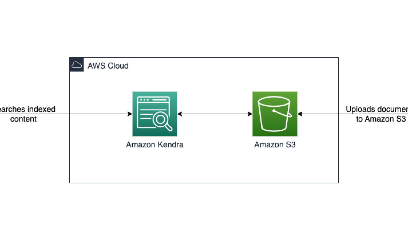
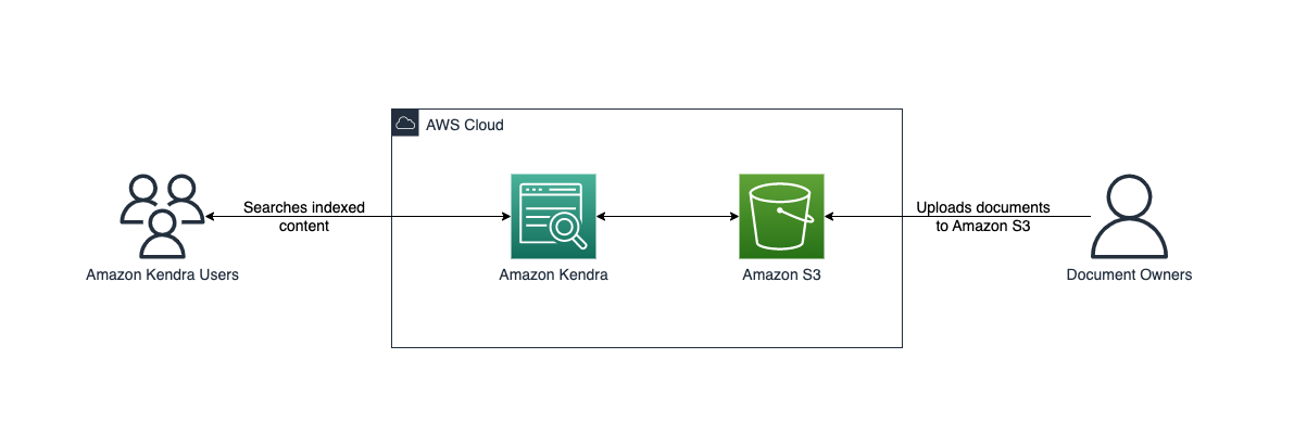
The CloudFormation template sets up an Amazon Kendra data source with a connection to Amazon S3. The template also creates one role for the Amazon Kendra data source service. You can specify an S3 bucket, synchronization schedule, and inclusion/exclusion patterns. When the synchronization job has finished, you can search the indexed content through the Search console. The following diagram illustrates this workflow.

This post guides you to the following steps:

1. Deploy the provided template.
2. Upload the documents to the S3 bucket that you create. If you provide a bucket with documents, you can omit this step.
3. Wait until the index finishes crawling the data source.

Prerequisites

For this walkthrough, you should have the following prerequisites:

• An AWS account where the proposed solution can be deployed.
• An Amazon Kendra index for attaching a data source to the stack.
• The set of documents that are used to create the Amazon Kendra index. In this solution, you are using a compressed file of AWS whitepapers.

Deploy the solution with AWS CloudFormation

To deploy the CloudFormation template, complete the following steps:

1. Choose
   

You’re redirected to the AWS CloudFormation console.

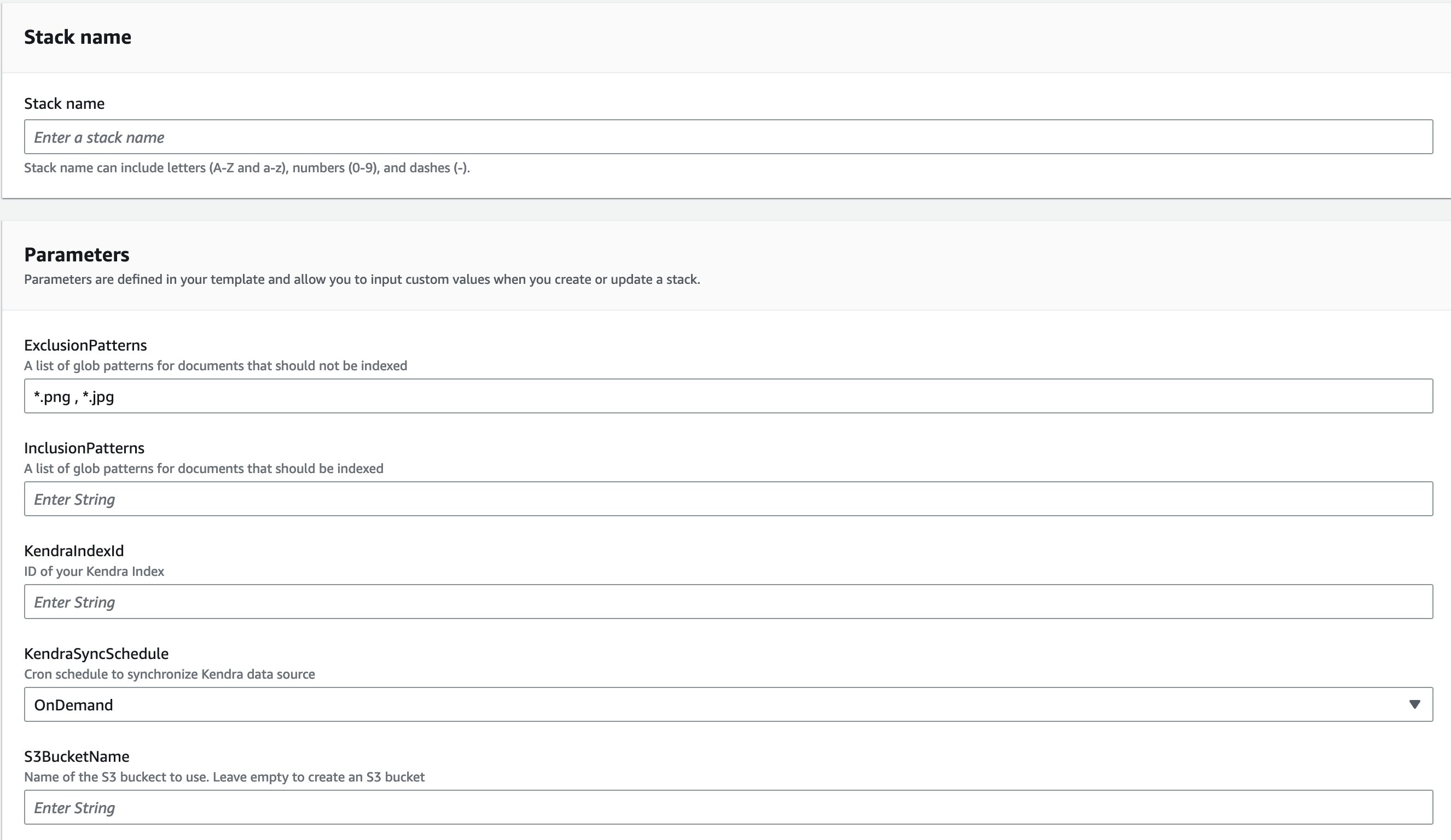
2. You can modify the parameters or use the default values:
   • The Amazon Kendra data source name is automatically set using the stack name and associated bucket name.
   • For KendraIndexId, enter the Amazon Kendra index ID where you will attach the data source.
   • You can also choose when you want to run the data source synchronization using KendraSyncSchedule. By default, it’s set to OnDemand.
   • For S3BucketName, you can either enter a bucket you have already created or leave it empty. If you leave it empty, a bucket will be created for you. Either way, the bucket is used as the Amazon Kendra data source. For this post, we leave it empty.

It takes around 5 minutes for the stack to deploy the Amazon Kendra data source attached to the Amazon Kendra index.

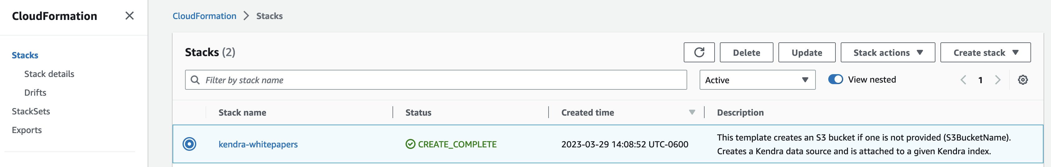
3. On the Outputs tab of the CloudFormation stack, copy the name of the created bucket, data source name, and ID.

The created stack deploys one role: <stack-name>-KendraDataSourceRole. It’s a best practice to deploy a role for each data source you create. This role gives Amazon Kendra data source to add or remove files from Amazon Kendra index, to get objects from Amazon S3 bucket.

Upload files to the S3 bucket

Amazon Kendra can handle multiple document types, such as .html, .pdf, .csv, .json, .docx, and .ppt. You can also have a combination of documents on a single index. The text contained in those documents is indexed to the provided Amazon Kendra index. You can search for keywords on AWS topics on best practices, databases, machine learning, security, and more using over 60 pdf files that you can download. For example, if you want to know where you can find more information about caching in the AWS whitepapers, Amazon Kendra can help you find documents related to databases and best practices.

When you download the AWS Whitepapers.zip file and uncompress the file, you see these six folders: Best_Practices, Databases, General, Machine_Learning, Security, Well_Architected. Upload these folders to your S3 bucket.

Synchronize the Amazon Kendra data source

Amazon Kendra data source data can synchronize your data based on preconfigured schedule or can be be manually triggered on-demand. By default, CloudFormation template configures the data source to on-demand synchronization schedule to be triggered manually as required.

To manually trigger the synchronization job from the AWS Amazon Kendra console, navigate to the Amazon Kendra index used as part of CloudFormation stack deployment, under Data Management in the navigation pane, choose Data Sources and then choose Sync now. This makes the S3 bucket synchronize with the data source.

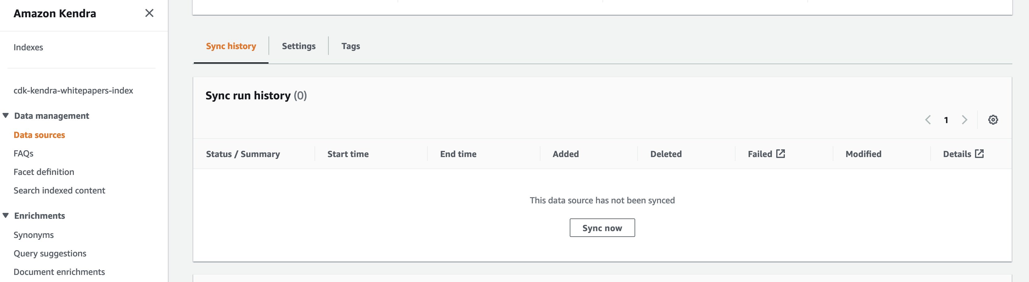
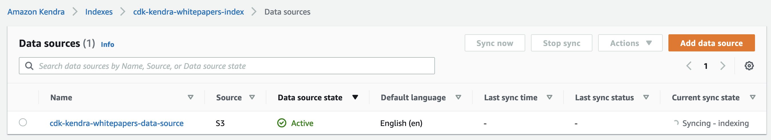
When the Amazon Kendra data source starts syncing, you should see the Current sync state as Syncing.

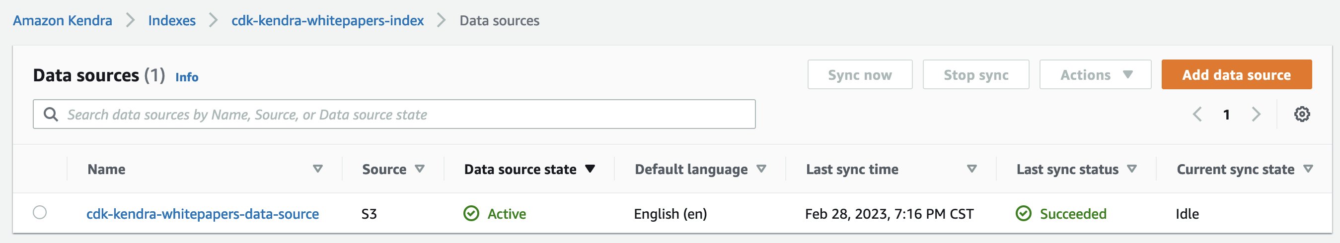
When the data source has finished, the Last sync status appears as Succeeded and Current sync state as Idle. You can now search the indexed content.

Configure synchronization schedule

The template allows you to run the schedule every hour at minute 0, for example, 13:00, 14:00, or 15:00. You also have the option to run it daily at 00:00 UTC. The Weekly setting runs Mondays at 00:00 UTC, and the Monthly setting runs every first day of the month at 00:00 UTC.

To change the schedule after the Amazon Kendra data source has been created, on the Actions menu, choose Edit. Under Configure sync settings, you find the Sync rule schedule section.

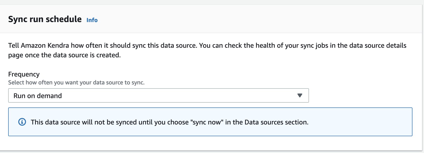
Under Frequency, you can select hourly, daily, weekly, monthly, or custom, all of which allow you to schedule your sync down to the minute.

Add exclusion patterns

The provided CloudFormation template allows you to add exclusion patterns. By default, .png and .jpg files will be added to the ExclusionPatterns parameter. Additional file formats can be added as a comma separated list to the exclusion pattern. Similarly, InclusionPatterns parameter may be used add comma list file formats to set up an inclusion pattern. If you don’t provide an inclusion pattern, all files are indexed except for the ones included in the exclusion parameter.

Clean up

To avoid costs, you can delete the stack from the AWS CloudFormation console. On the Stacks page, select the stack you created, choose Delete, and confirm the deletion of the stack.

If you haven’t provided a S3 bucket, the stack creates a bucket. If the bucket is empty, it’s automatically deleted. Otherwise, you need to empty the folder and manually delete it. If you provided a bucket, even if it’s empty, it won’t be deleted. Amazon Kendra index won’t be deleted. Only the Amazon Kendra data source created by the stack will be deleted.

Conclusion

In this post, we provided an CloudFormation template to easily synchronize your text documents on an S3 bucket to your Amazon Kendra index. This solution is helpful if you have multiple S3 buckets you want to index because you can create all the necessary components to query the documents with a few clicks in a consistent and repeatable manner. You can also see how image-based text documents can be handled in Amazon Kendra. To learn more about specific schedule patterns, refer to Schedule Expressions for Rules.

Leave a comment and learn more about Amazon Kendra index creation in the following Amazon Kendra Essentials+ workshop.

Special thanks to Jose Mauricio Mani Yanez for his help creating the example code and compiling the content for this post.

About the author

Rajesh Kumar Ravi is an AI/ML Specialist Solutions Architect at Amazon Web Services specializing in intelligent document search with Amazon Kendra and generative AI. He is a builder and problem solver, and contributes to development of new ideas. He enjoys walking and loves to go on short hiking trips outside of work.

Read More

You can now register machine learning (ML) models built in Amazon SageMaker Canvas with a single click to the Amazon SageMaker Model Registry, enabling you to operationalize ML models in production. Canvas is a visual interface that enables business analysts to generate accurate ML predictions on their own—without requiring any ML experience or having to write a single line of code. Although it’s a great place for development and experimentation, to derive value from these models, they need to be operationalized—namely, deployed in a production environment where they can be used to make predictions or decisions. Now with the integration with the model registry, you can store all model artifacts, including metadata and performance metrics baselines, to a central repository and plug them into your existing model deployment CI/CD processes.

The model registry is a repository that catalogs ML models, manages various model versions, associates metadata (such as training metrics) with a model, manages the approval status of a model, and deploys them to production. After you create a model version, you typically want to evaluate its performance before you deploy it to a production endpoint. If it performs to your requirements, you can update the approval status of the model version to approved. Setting the status to approved can initiate CI/CD deployment for the model. If the model version doesn’t perform to your requirements, you can update the approval status to rejected in the registry, which prevents the model from being deployed into an escalated environment.

A model registry plays a key role in the model deployment process because it packages all model information and enables the automation of model promotion to production environments. The following are some ways that a model registry can help in operationalizing ML models:

• Version control – A model registry allows you to track different versions of your ML models, which is essential when deploying models in production. By keeping track of model versions, you can easily revert to a previous version if a new version causes issues.
• Collaboration – A model registry enables collaboration among data scientists, engineers, and other stakeholders by providing a centralized location for storing, sharing, and accessing models. This can help streamline the deployment process and ensure that everyone is working with the same model.
• Governance – A model registry can help with compliance and governance by providing an auditable history of model changes and deployments.

Overall, a model registry can help streamline the process of deploying ML models in production by providing version control, collaboration, monitoring, and governance.

Overview of solution

For our use case, we are assuming the role of a business user in the marketing department of a mobile phone operator, and we have successfully created an ML model in Canvas to identify customers with the potential risk of churn. Thanks to the predictions generated by our model, we now want to move this from our development environment to production. However, before our model gets deployed to a production endpoint, it needs to be reviewed and approved by a central MLOps team. This team is responsible for managing model versions, reviewing all associated metadata (such as training metrics) with a model, managing the approval status of every ML model, deploying approved models to production, and automating model deployment with CI/CD. To streamline the process of deploying our model in production, we take advantage of the integration of Canvas with the model registry and register our model for review by our MLOps team.

The workflow steps are as follows:

1. Upload a new dataset with the current customer population into Canvas. For the full list of supported data sources, refer to Import data into Canvas.
2. Build ML models and analyze their performance metrics. Refer to the instructions to build a custom ML model in Canvas and evaluate the model’s performance.
3. Register the best performing versions to the model registry for review and approval.
4. Deploy the approved model version to a production endpoint for real-time inferencing.

You can perform Steps 1–3 in Canvas without writing a single line of code.

Prerequisites

For this walkthrough, make sure that the following prerequisites are met:

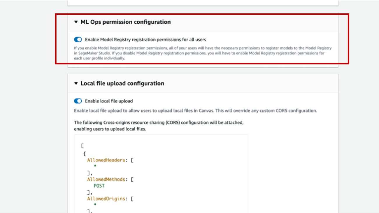
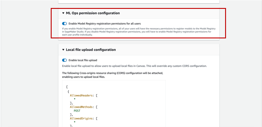
1. To register model versions to the model registry, the Canvas admin must give the necessary permissions to the Canvas user, which you can manage in the SageMaker domain that hosts your Canvas application. For more information, refer to the Amazon SageMaker Developer Guide. When granting your Canvas user permissions, you must choose whether to allow the user to register their model versions in the same AWS account.

2. Implement the prerequisites mentioned in Predict customer churn with no-code machine learning using Amazon SageMaker Canvas.

You should now have three model versions trained on historical churn prediction data in Canvas:

• V1 trained with all 21 features and quick build configuration with a model score of 96.903%
• V2 trained with all 19 features (removed phone and state features) and quick build configuration and improved accuracy of 97.403%
• V3 trained with standard build configuration with 97.03% model score
  

Use the customer churn prediction model

Enable Show advanced metrics and review the objective metrics associated with each model version so that we can select the best performing model for registration to the model registry.

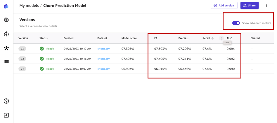
Based on the performance metrics, we select version 2 to be registered.

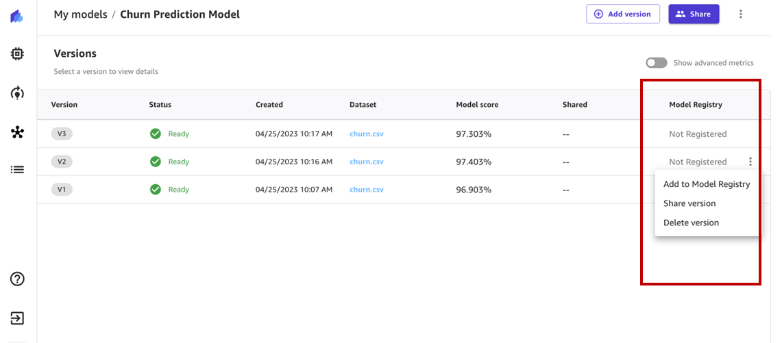
The model registry tracks all the model versions that you train to solve a particular problem in a model group. When you train a Canvas model and register it to the model registry, it gets added to a model group as a new model version.

At the time of registration, a model group within the model registry is automatically created. Optionally, you can rename it to a name of your choice or use an existing model group in the model registry.

For this example, we use the autogenerated model group name and choose Add.

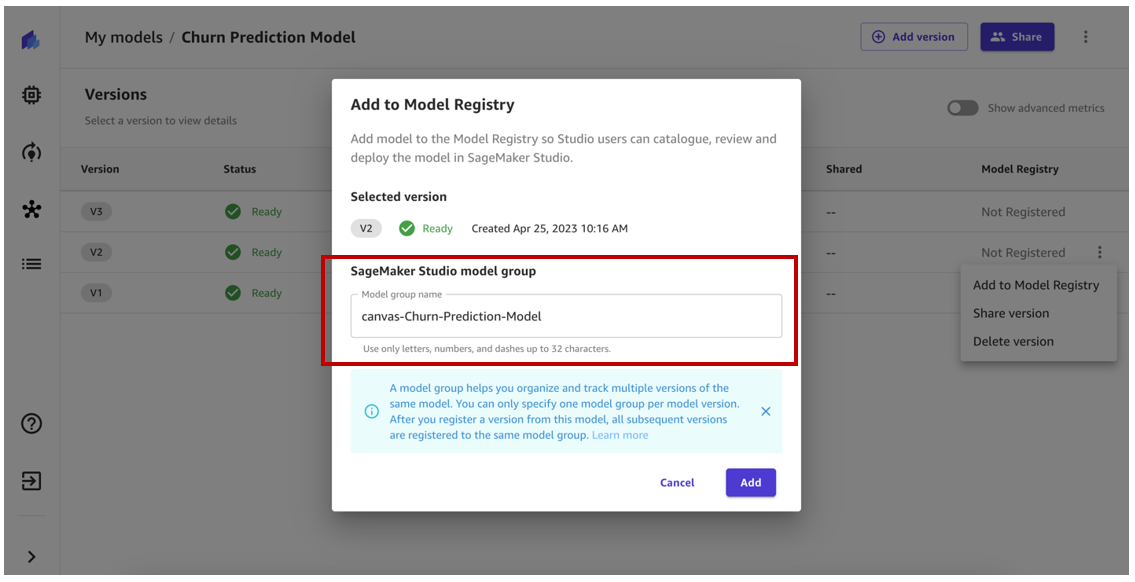
Our model version should now be registered to the model group in the model registry. If we were to register another model version, it would be registered to the same model group.

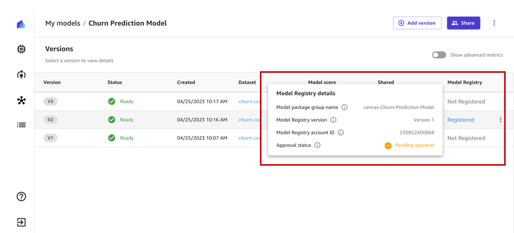
The status of the model version should have changed from Not Registered to Registered.

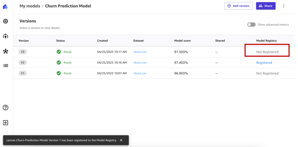
When we hover over the status, we can review the model registry details, which include the model group name, model registry account ID, and approval status. Right after registration, the status changes to Pending Approval, which means that this model is registered in the model registry but is pending review and approval from a data scientist or MLOps team member and can only be deployed to an endpoint if approved.

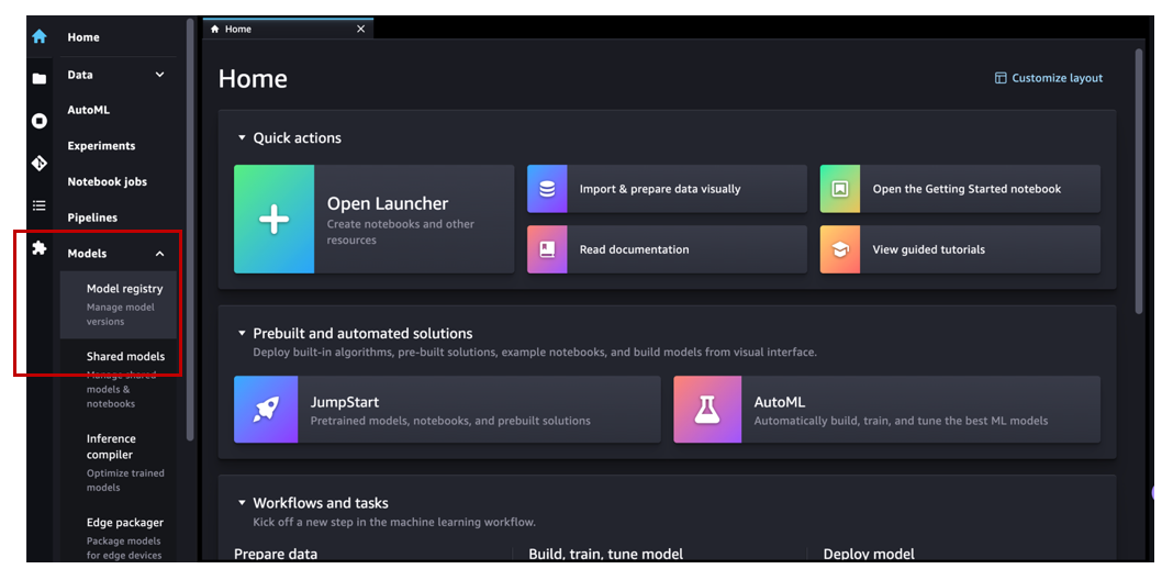
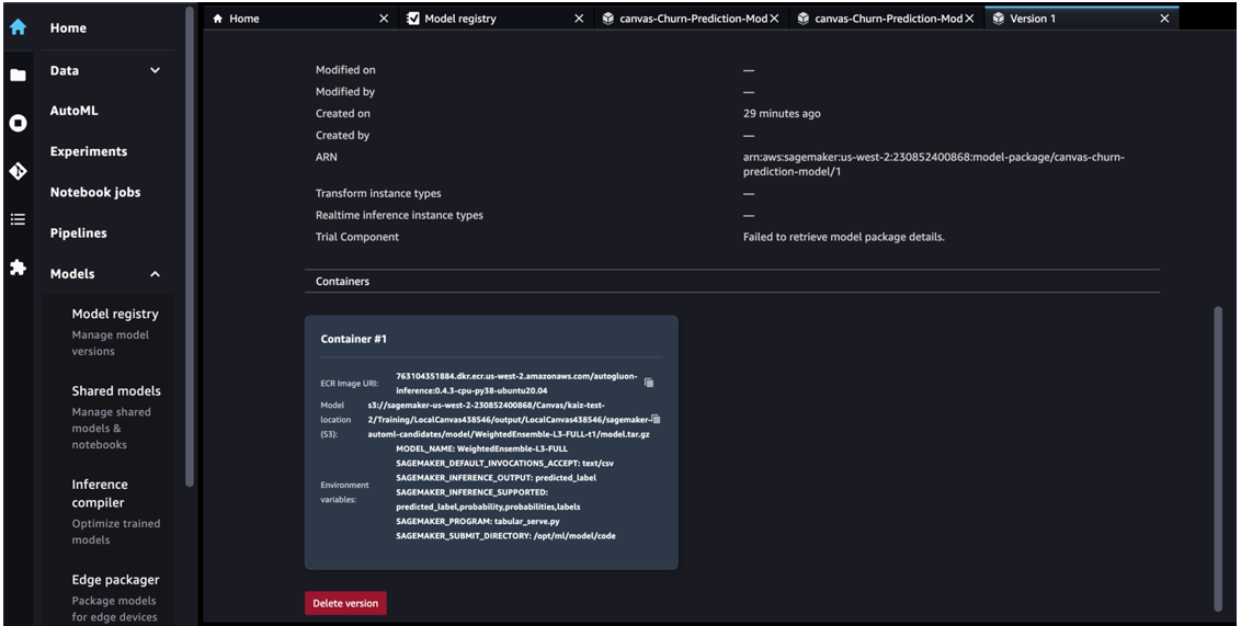
Now let’s navigate to Amazon SageMaker Studio and assume the role of an MLOps team member. Under Models in the navigation pane, choose Model registry to open the model registry home page.

We can see the model group canvas-Churn-Prediction-Model that Canvas automatically created for us.

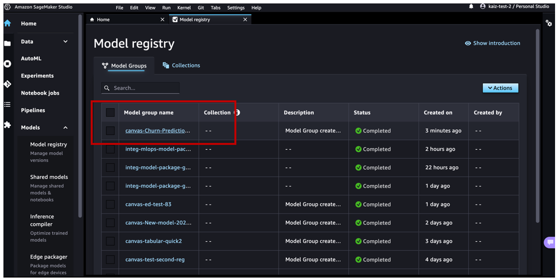
Choose the model to review all the versions registered to this model group and then review the corresponding model details.

If you open the details for version 1, we can see that the Activity tab keeps track of all the events happening on the model.

On the Model quality tab, we can review the model metrics, precision/recall curves, and confusion matrix plots to understand the model performance.

On the Explainability tab, we can review the features that influenced the model’s performance the most.

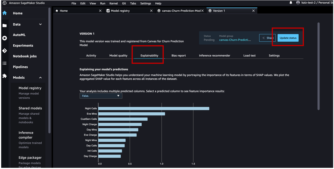
After we have reviewed the model artifacts, we can change the approval status from Pending to Approved.

We can now see the updated activity.

The Canvas business user will now be able to see that the registered model status changed from Pending Approval to Approved.

As the MLOps team member, because we have approved this ML model, let’s deploy it to an endpoint.

In Studio, navigate to the model registry home page and choose the canvas-Churn-Prediction-Model model group. Choose the version to be deployed and go to the Settings tab.

Browse to get the model package ARN details from the selected model version in the model registry.

Open a notebook in Studio and run the following code to deploy the model to an endpoint. Replace the model package ARN with your own model package ARN.

from sagemaker import ModelPackage
from time import gmtime, strftime
import boto3
import os
import pandas as pd
import sagemaker
import time
from datetime import datetime
from sagemaker import ModelPackage

boto_session = boto3.session.Session()
sagemaker_client = boto_session.client("sagemaker")
sagemaker_session = sagemaker.session.Session(
boto_session=boto_session, sagemaker_client=sagemaker_client
)
role=(sagemaker.get_execution_role())
model_package_arn = 'arn:aws:sagemaker:us-west-2:1234567890:model-package/canvas-churn-prediction-model/3'
model = ModelPackage(role=role,
model_package_arn=model_package_arn,
sagemaker_session=sagemaker_session)
model.deploy(initial_instance_count=1, instance_type='ml.m5.xlarge')

After the endpoint gets created, you can see it tracked as an event on the Activity tab of the model registry.

You can double-click on the endpoint name to get its details.

Now that we have an endpoint, let’s invoke it to get a real-time inference. Replace your endpoint name in the following code snippet:

import boto3, sys

endpoint_name = '3-2342-12-21-12-07-09-075'
sm_rt = boto3.Session().client('runtime.sagemaker')

payload = [163, 806, 'no', 'yes', 300, 8.162204, 3, 3.933, 2.245779, 4, 6.50863, 6.05194, 5, 4.948816088, 1.784764, 2, 5.135322, 8]
l = ",".join([str(p) for p in payload])

response = sm_rt.invoke_endpoint(EndpointName=endpoint_name, ContentType='text/csv', Accept='text/csv', Body=l)

response = response['Body'].read().decode("utf-8")
print(response)

Clean up

To avoid incurring future charges, delete the resources you created while following this post. This includes logging out of Canvas and deleting the deployed SageMaker endpoint. Canvas bills you for the duration of the session, and we recommend logging out of Canvas when you’re not using it. Refer to Logging out of Amazon SageMaker Canvas for more details.

Conclusion

In this post, we discussed how Canvas can help operationalize ML models to production environments without requiring ML expertise. In our example, we showed how an analyst can quickly build a highly accurate predictive ML model without writing any code and register it to the model registry. The MLOps team can then review it and either reject the model or approve the model and initiate the downstream CI/CD deployment process.

To start your low-code/no-code ML journey, refer to Amazon SageMaker Canvas.

Special thanks to everyone who contributed to the launch:

Backend:

• Huayuan (Alice) Wu
• Krittaphat Pugdeethosapol
• Yanda Hu
• John He
• Esha Dutta
• Prashanth

Front end:

• Kaiz Merchant
• Ed Cheung

About the Authors

Janisha Anand is a Senior Product Manager in the SageMaker Low/No Code ML team, which includes SageMaker Autopilot. She enjoys coffee, staying active, and spending time with her family.

Krittaphat Pugdeethosapol is a Software Development Engineer at Amazon SageMaker and mainly works with SageMaker low-code and no-code products.

Huayuan(Alice) Wu is a Software Development Engineer at Amazon SageMaker. She focuses on building ML tools and products for customers. Outside of work, she enjoys the outdoors, yoga, and hiking.

Read More

Today, data scientists who are training deep learning models need to identify and remediate model training issues to meet accuracy targets for production deployment, and require a way to utilize standard tools for debugging model training. Among the data scientist community, TensorBoard is a popular toolkit that allows data scientists to visualize and analyze various aspects of their machine learning (ML) models and training processes. It provides a suite of tools for visualizing training metrics, examining model architectures, exploring embeddings, and more. TensorFlow and PyTorch projects both endorse and use TensorBoard in their official documentation and examples.

Amazon SageMaker with TensorBoard is a capability that brings the visualization tools of TensorBoard to SageMaker. Integrated with SageMaker training jobs and domains, it provides SageMaker domain users access to the TensorBoard data and helps domain users perform model debugging tasks using the SageMaker TensorBoard visualization plugins. When they create a SageMaker training job, domain users can use TensorBoard using the SageMaker Python SDK or Boto3 API. SageMaker with TensorBoard is supported by the SageMaker Data Manager plugin, with which domain users can access many training jobs in one place within the TensorBoard application.

In this post, we demonstrate how to set up a training job with TensorBoard in SageMaker using the SageMaker Python SDK, access SageMaker TensorBoard, explore training output data visualized in TensorBoard, and delete unused TensorBoard applications.

Solution overview

A typical training job for deep learning in SageMaker consists of two main steps: preparing a training script and configuring a SageMaker training job launcher. In this post, we walk you through the required changes to collect TensorBoard-compatible data from SageMaker training.

Prerequisites

To start using SageMaker with TensorBoard, you need to set up a SageMaker domain with an Amazon VPC under an AWS account. Domain user profiles for each individual user are required to access the TensorBoard on SageMaker, and the AWS Identity and Access Management (IAM) execution role needs a minimum set of permissions, including the following:

• sagemaker:CreateApp
• sagemaker:DeleteApp
• sagemaker:DescribeTrainingJob
• sagemaker:Search
• s3:GetObject
• s3:ListBucket

For more information on how to set up SageMaker Domain and user profiles, see Onboard to Amazon SageMaker Domain Using Quick setup and Add and Remove User Profiles.

Directory structure

When using Amazon SageMaker Studio, the directory structure can be organized as follows:

.
├── script
│	└── train.py
└── simple_tensorboard.ipynb

Here, script/train.py is your training script, and simple_tensorboard.ipynb launches the SageMaker training job.

Modify your training script

You can use any of the following tools to collect tensors and scalars: TensorBoardX, TensorFlow Summary Writer, PyTorch Summary Writer, or Amazon SageMaker Debugger, and specify the data output path as the log directory in the training container (log_dir). In this sample code, we use TensorFlow to train a simple, fully connected neural network for a classification task. For other options, refer to Prepare a training job with a TensorBoard output data configuration. In the train() function, we use the tensorflow.keras.callbacks.TensorBoard tool to collect tensors and scalars, specify /opt/ml/output/tensorboard as the log directory in the training container, and pass it to model training callbacks argument. See the following code:

import argparse
import json
import tensorflow as tf


def parse_args():
    cmdline = argparse.ArgumentParser(
        formatter_class=argparse.ArgumentDefaultsHelpFormatter
    )
    cmdline.add_argument("--epochs", default=5, type=int, help="""Number of epochs.""")
    cmdline.add_argument(
        "--optimizer", default="adam", type=str, help="""Optimizer type"""
    )
    cmdline.add_argument(
        "--loss",
        default="sparse_categorical_crossentropy",
        type=str,
        help="""Optimizer type""",
    )
    cmdline.add_argument(
        "--metrics",
        action="store",
        dest="metrics",
        type=json.loads,
        default="['accuracy']",
        help="List of metrics to be evaluated by the model during training and testing.",
    )
    return cmdline


def create_model():
    return tf.keras.models.Sequential(
        [
            tf.keras.layers.Flatten(input_shape=(28, 28)),
            tf.keras.layers.Dense(512, activation="relu"),
            tf.keras.layers.Dropout(0.2),
            tf.keras.layers.Dense(10, activation="softmax"),
        ]
    )


def train(args):
    mnist = tf.keras.datasets.mnist
    (x_train, y_train), (x_test, y_test) = mnist.load_data()
    x_train, x_test = x_train / 255.0, x_test / 255.0

    model = create_model()
    model.compile(optimizer=args.optimizer, loss=args.loss, metrics=args.metrics)

    # setup TensorBoard Callback
    LOG_DIR = "/opt/ml/output/tensorboard"
    tensorboard_callback = tf.keras.callbacks.TensorBoard(
        log_dir=LOG_DIR,
        histogram_freq=1,
        update_freq=1,
        embeddings_freq=5,
        write_images=True,
    )

    # pass TensorBoard Callback into the Model fit
    model.fit(
        x=x_train,
        y=y_train,
        epochs=args.epochs,
        validation_data=(x_test, y_test),
        callbacks=[tensorboard_callback],
    )


if __name__ == "__main__":
    cmdline = parse_args()
    args, unknown_args = cmdline.parse_known_args()
    train(args)

Construct a SageMaker training launcher with a TensorBoard data configuration

Use sagemaker.debugger.TensorBoardOutputConfig while configuring a SageMaker framework estimator, which maps the Amazon Simple Storage Service (Amazon S3) bucket you specify for saving TensorBoard data with the local path in the training container (for example, /opt/ml/output/tensorboard). You can use a different container local output path. However, it must be consistent with the value of the LOG_DIR variable, as specified in the previous step, to have SageMaker successfully search the local path in the training container and save the TensorBoard data to the S3 output bucket.

Next, pass the object of the module to the tensorboard_output_config parameter of the estimator class. The following code snippet shows an example of preparing a TensorFlow estimator with the TensorBoard output configuration parameter.

The following is the boilerplate code:

import os
from datetime import datetime
import boto3
import sagemaker

time_str = datetime.now().strftime("%d-%m-%Y-%H-%M-%S")

region = boto3.session.Session().region_name
boto_sess = boto3.Session()
role = sagemaker.get_execution_role()
sm = sagemaker.Session()

base_job_name = "simple-tensorboard"
date_str = datetime.now().strftime("%d-%m-%Y")
time_str = datetime.now().strftime("%d-%m-%Y-%H-%M-%S")
job_name = f"{base_job_name}-{time_str}"

s3_output_bucket = os.path.join("s3://", sm.default_bucket(), base_job_name)

output_path = os.path.join(s3_output_bucket, "sagemaker-output", date_str, job_name)
code_location = os.path.join(s3_output_bucket, "sagemaker-code", date_str, job_name)

The following code is for the training container:

instance_type = "ml.c5.xlarge"
instance_count = 1

image_uri = sagemaker.image_uris.retrieve(
    framework="tensorflow",
    region=region,
    version="2.11",
    py_version="py39",
    image_scope="training",
    instance_type=instance_type,
)

The following code is the TensorBoard configuration:

from sagemaker.tensorflow import TensorFlow

tensorboard_output_config = sagemaker.debugger.TensorBoardOutputConfig(
    s3_output_path=os.path.join(output_path, "tensorboard"),
    container_local_output_path="/opt/ml/output/tensorboard",
)

hyperparameters = {
    "epochs": 5,
    "optimizer": "adam",
    "loss": "sparse_categorical_crossentropy",
    "metrics": "'["accuracy"]'",
}

estimator = TensorFlow(
    entry_point="train.py",
    source_dir="script",
    role=role,
    image_uri=image_uri,
    instance_count=1,
    instance_type="ml.c5.xlarge",
    base_job_name=job_name,
    tensorboard_output_config=tensorboard_output_config,
    hyperparameters=hyperparameters,
)

Launch the training job with the following code:

estimator.fit(
    inputs=None,
    wait=False,
    job_name=job_name,
)

Access TensorBoard on SageMaker

You can access TensorBoard with two methods: programmatically using the sagemaker.interactive_apps.tensorboard module that generates the URL or using the TensorBoard landing page on the SageMaker console. After you open TensorBoard, SageMaker runs the TensorBoard plugin and automatically finds and loads all training job output data in a TensorBoard-compatible file format from S3 buckets paired with training jobs during or after training.

The following code autogenerates the URL to the TensorBoard console landing page:

from sagemaker.interactive_apps import tensorboard
app = tensorboard.TensorBoardApp(region)

print("Navigate to the following URL:")
if app._is_studio_user:
    print(app.get_app_url(job_name))
else:
    print(app.get_app_url())

This returns the following message with a URL that opens the TensorBoard landing page.

>>> Navigate to the following URL: https://<sagemaker_domain_id>.studio.<region>.sagemaker.aws/tensorboard/default/data/plugin/sa

For opening TensorBoard from the SageMaker console, please refer to How to access TensorBoard on SageMaker.

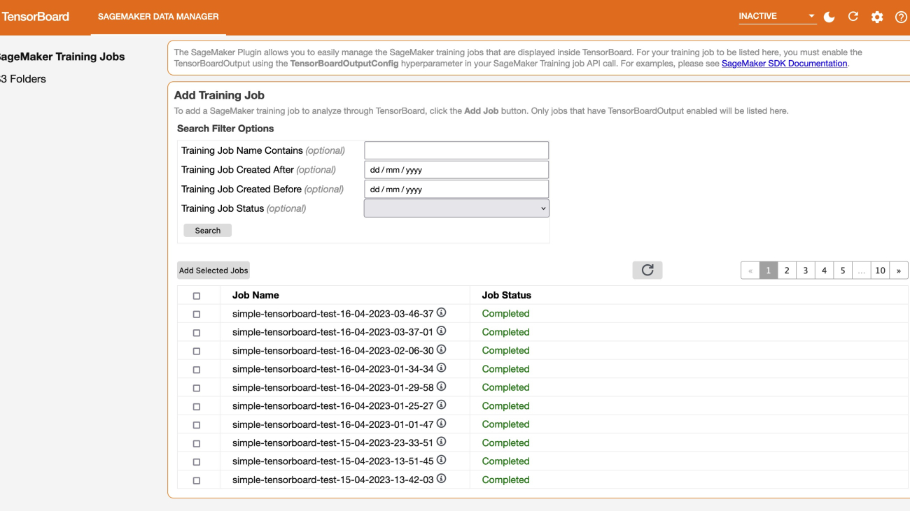
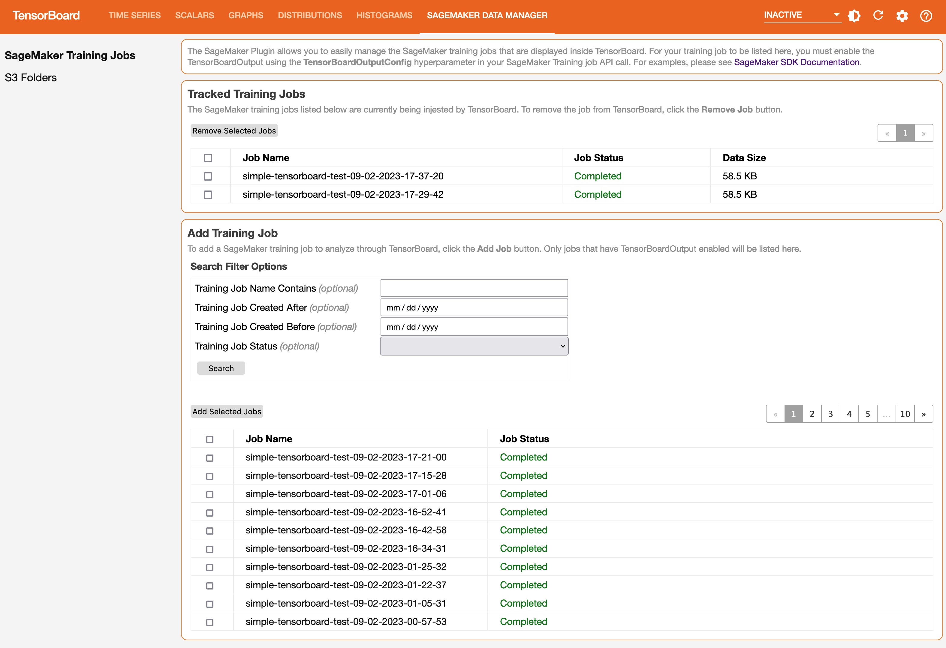
When you open the TensorBoard application, TensorBoard opens with the SageMaker Data Manager tab. The following screenshot shows the full view of the SageMaker Data Manager tab in the TensorBoard application.

On the SageMaker Data Manager tab, you can select any training job and load TensorBoard-compatible training output data from Amazon S3.

1. In the Add Training Job section, use the check boxes to choose training jobs from which you want to pull data and visualize for debugging.
2. Choose Add Selected Jobs.

The selected jobs should appear in the Tracked Training Jobs section.

Refresh the viewer by choosing the refresh icon in the upper-right corner, and the visualization tabs should appear after the job data is successfully loaded.

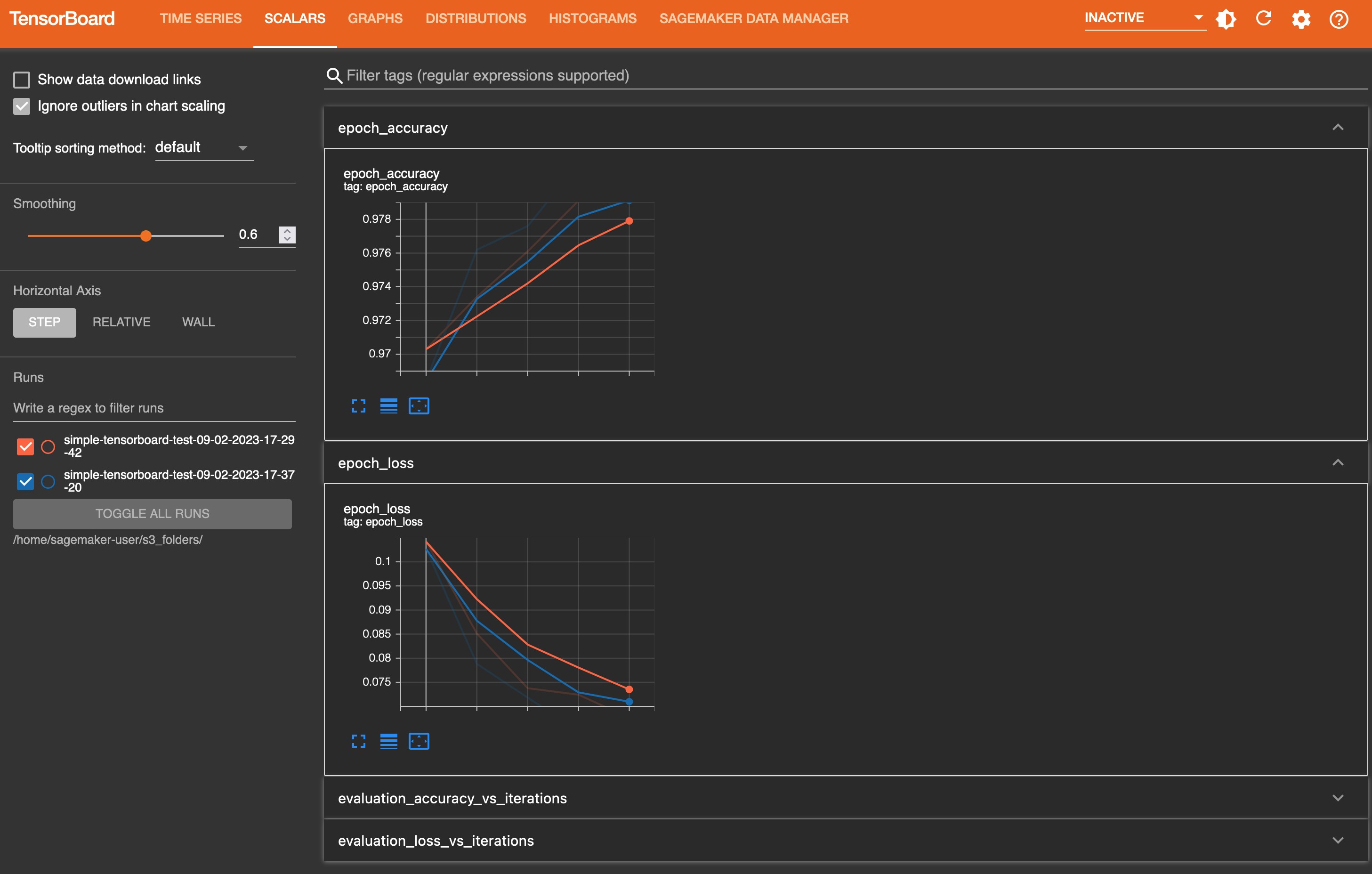
Explore training output data visualized in TensorBoard

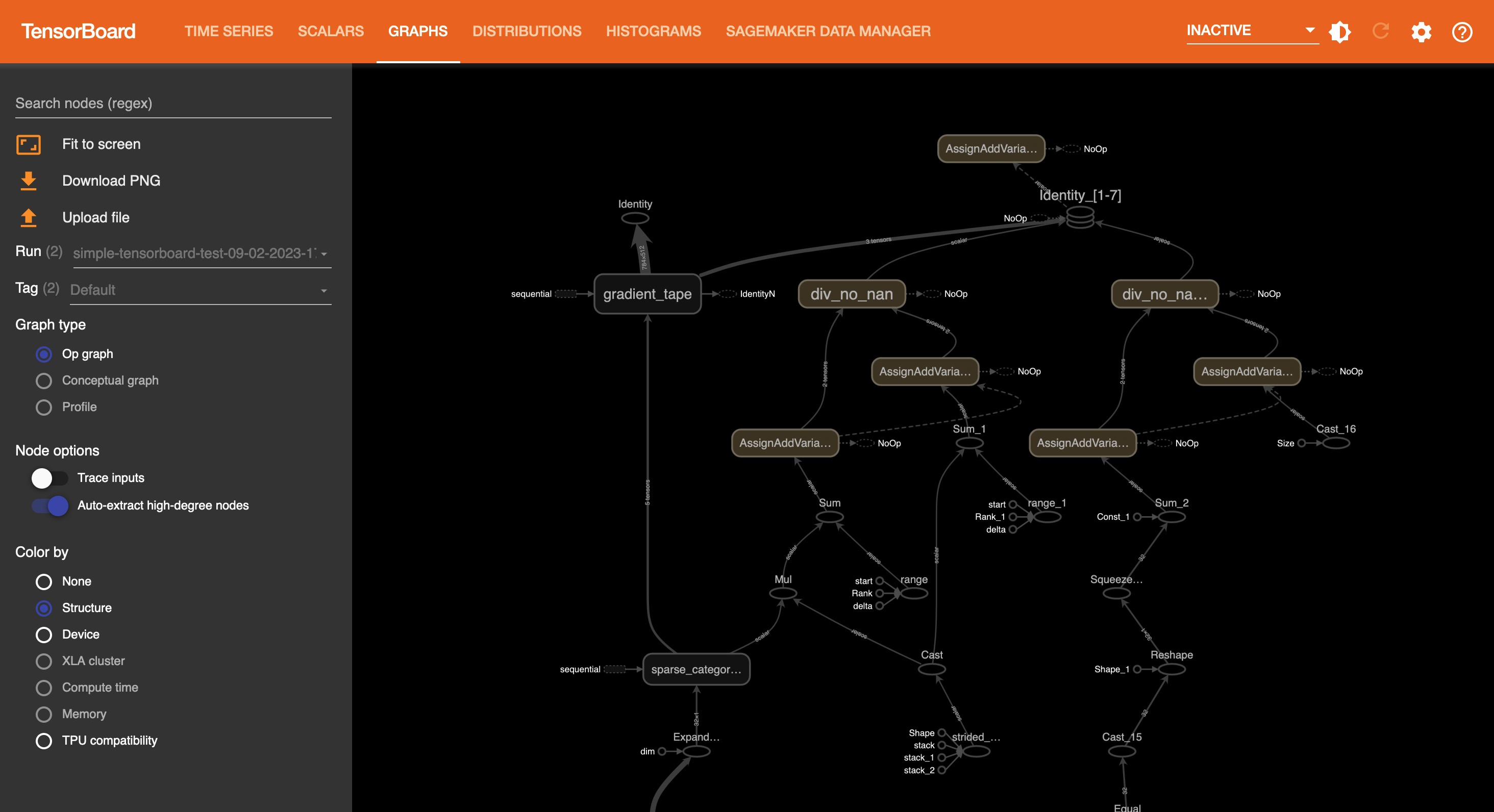
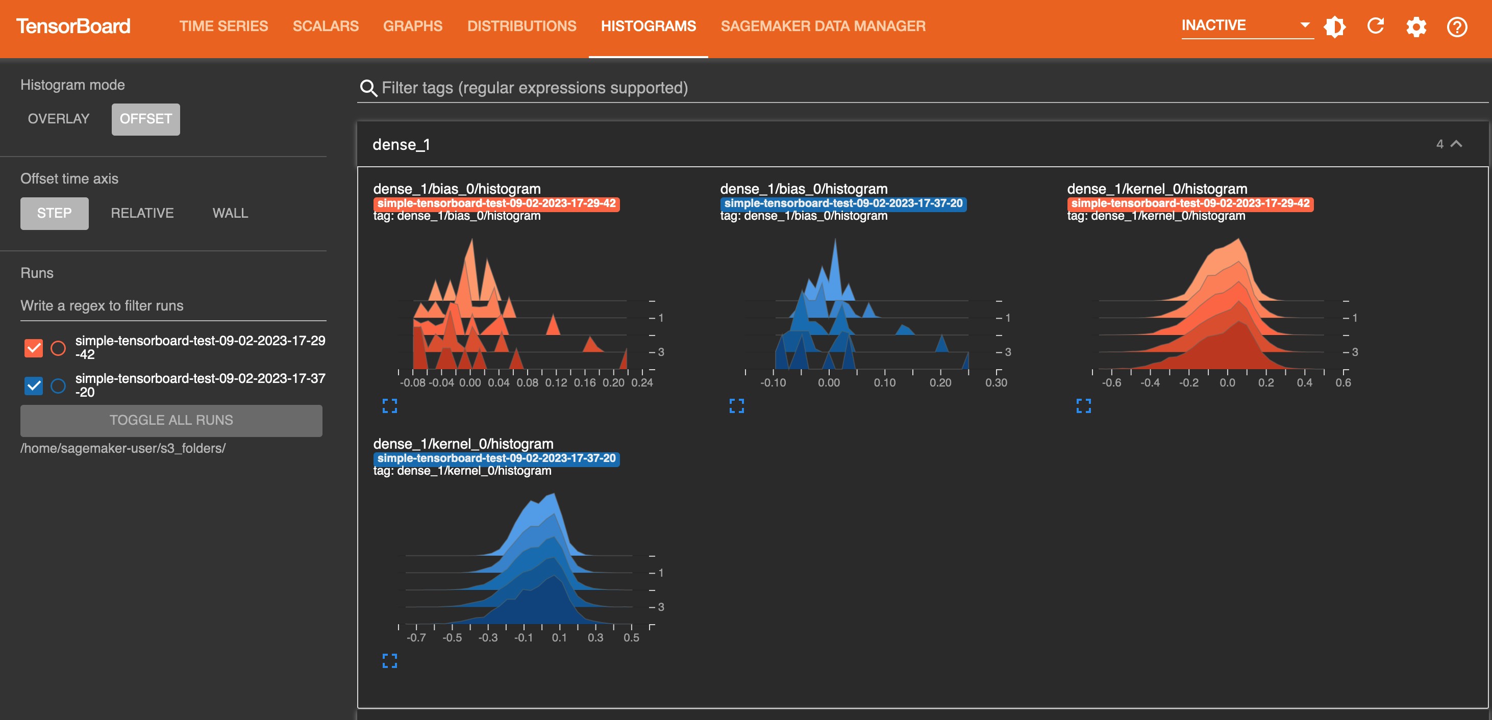
On the Time Series tab and other graphics-based tabs, you can see the list of Tracked Training Jobs in the left pane. You can also use the check boxes of the training jobs to show or hide visualizations. The TensorBoard dynamic plugins are activated dynamically depending on how you have set your training script to include summary writers and pass callbacks for tensor and scalar collection, and the graphics tabs also appear dynamically. The following screenshots show example views of each tab with visualizations of the collected metrics of two training jobs. The metrices include time series, scalar, graph, distribution, and histogram plugins.

The following screenshot is the Time Series tab view.

The following screenshot is the Scalars tab view.

The following screenshot is the Graphs tab view.

The following screenshot is the Distributions tab view.

The following screenshot is the Histograms tab view.

Clean up

After you are done with monitoring and experimenting with jobs in TensorBoard, shut the TensorBoard application down:

1. On the SageMaker console, choose Domains in the navigation pane.
2. Choose your domain.
3. Choose your user profile.
4. Under Apps, choose Delete App for the TensorBoard row.
5. Choose Yes, delete app.
6. Enter delete in the text box, then choose Delete.

A message should appear at the top of the page: “Default is being deleted”.

Conclusion

TensorBoard is a powerful tool for visualizing, analyzing, and debugging deep learning models. In this post, we provide a guide to using SageMaker with TensorBoard, including how to set up TensorBoard in a SageMaker training job using the SageMaker Python SDK, access SageMaker TensorBoard, explore training output data visualized in TensorBoard, and delete unused TensorBoard applications. By following these steps, you can start using TensorBoard in SageMaker for your work.

We encourage you to experiment with different features and techniques.

About the authors

Dr. Baichuan Sun is a Senior Data Scientist at AWS AI/ML. He is passionate about solving strategic business problems with customers using data-driven methodology on the cloud, and he has been leading projects in challenging areas including robotics computer vision, time series forecasting, price optimization, predictive maintenance, pharmaceutical development, product recommendation system, etc. In his spare time he enjoys traveling and hanging out with family.

Manoj Ravi is a Senior Product Manager for Amazon SageMaker. He is passionate about building next-gen AI products and works on software and tools to make large-scale machine learning easier for customers. He holds an MBA from Haas School of Business and a Masters in Information Systems Management from Carnegie Mellon University. In his spare time, Manoj enjoys playing tennis and pursuing landscape photography.

Read More