Posts in category: Amazon AWS

This post is co-written with Mahima Agarwal, Machine Learning Engineer, and Deepak Mettem, Senior Engineering Manager, at VMware Carbon Black

VMware Carbon Black is a renowned security solution offering protection against the full spectrum of modern cyberattacks. With terabytes of data generated by the product, the security analytics team focuses on building machine learning (ML) solutions to surface critical attacks and spotlight emerging threats from noise.

It is critical for the VMware Carbon Black team to design and build a custom end-to-end MLOps pipeline that orchestrates and automates workflows in the ML lifecycle and enables model training, evaluations, and deployments.

There are two main purposes for building this pipeline: support the data scientists for late-stage model development, and surface model predictions in the product by serving models in high volume and in real-time production traffic. Therefore, VMware Carbon Black and AWS chose to build a custom MLOps pipeline using Amazon SageMaker for its ease of use, versatility, and fully managed infrastructure. We orchestrate our ML training and deployment pipelines using Amazon Managed Workflows for Apache Airflow (Amazon MWAA), which enables us to focus more on programmatically authoring workflows and pipelines without having to worry about auto scaling or infrastructure maintenance.

With this pipeline, what once was Jupyter notebook-driven ML research is now an automated process deploying models to production with little manual intervention from data scientists. Earlier, the process of training, evaluating, and deploying a model could take over a day; with this implementation, everything is just a trigger away and has reduced the overall time to few minutes.

In this post, VMware Carbon Black and AWS architects discuss how we built and managed custom ML workflows using Gitlab, Amazon MWAA, and SageMaker. We discuss what we achieved so far, further enhancements to the pipeline, and lessons learned along the way.

Solution overview

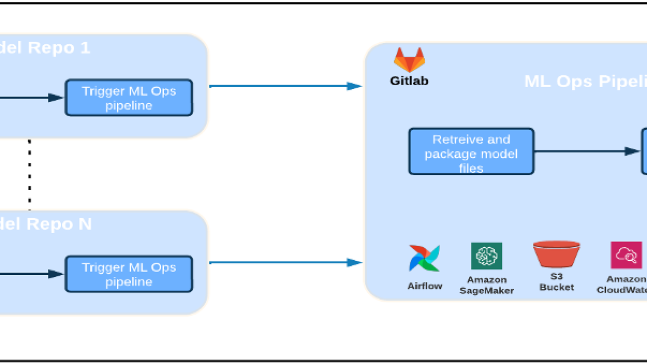
The following diagram illustrates the ML platform architecture.

High level Solution Design

This ML platform was envisioned and designed to be consumed by different models across various code repositories. Our team uses GitLab as a source code management tool to maintain all the code repositories. Any changes in the model repository source code are continuously integrated using the Gitlab CI, which invokes the subsequent workflows in the pipeline (model training, evaluation, and deployment).

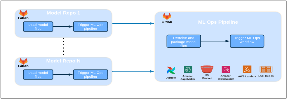
The following architecture diagram illustrates the end-to-end workflow and the components involved in our MLOps pipeline.

End-To-End Workflow

The ML model training, evaluation, and deployment pipelines are orchestrated using Amazon MWAA, referred to as a Directed Acyclic Graph (DAG). A DAG is a collection of tasks together, organized with dependencies and relationships to say how they should run.

At a high level, the solution architecture includes three main components:

• ML pipeline code repository
• ML model training and evaluation pipeline
• ML model deployment pipeline

Let’s discuss how these different components are managed and how they interact with each other.

ML pipeline code repository

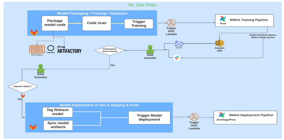
After the model repo integrates the MLOps repo as their downstream pipeline, and a data scientist commits code in their model repo, a GitLab runner does standard code validation and testing defined in that repo and triggers the MLOps pipeline based on the code changes. We use Gitlab’s multi-project pipeline to enable this trigger across different repos.

The MLOps GitLab pipeline runs a certain set of stages. It conducts basic code validation using pylint, packages the model’s training and inference code within the Docker image, and publishes the container image to Amazon Elastic Container Registry (Amazon ECR). Amazon ECR is a fully managed container registry offering high-performance hosting, so you can reliably deploy application images and artifacts anywhere.

ML model training and evaluation pipeline

After the image is published, it triggers the training and evaluation Apache Airflow pipeline through the AWS Lambda function. Lambda is a serverless, event-driven compute service that lets you run code for virtually any type of application or backend service without provisioning or managing servers.

After the pipeline is successfully triggered, it runs the Training and Evaluation DAG, which in turn starts the model training in SageMaker. At the end of this training pipeline, the identified user group gets a notification with the training and model evaluation results over email through Amazon Simple Notification Service (Amazon SNS) and Slack. Amazon SNS is fully managed pub/sub service for A2A and A2P messaging.

After meticulous analysis of the evaluation results, the data scientist or ML engineer can deploy the new model if the performance of the newly trained model is better compared to the previous version. The performance of the models is evaluated based on the model-specific metrics (such as F1 score, MSE, or confusion matrix).

ML model deployment pipeline

To start deployment, the user starts the GitLab job that triggers the Deployment DAG through the same Lambda function. After the pipeline runs successfully, it creates or updates the SageMaker endpoint with the new model. This also sends a notification with the endpoint details over email using Amazon SNS and Slack.

In the event of failure in either of the pipelines, users are notified over the same communication channels.

SageMaker offers real-time inference that is ideal for inference workloads with low latency and high throughput requirements. These endpoints are fully managed, load balanced, and auto scaled, and can be deployed across multiple Availability Zones for high availability. Our pipeline creates such an endpoint for a model after it runs successfully.

In the following sections, we expand on the different components and dive into the details.

GitLab: Package models and trigger pipelines

We use GitLab as our code repository and for the pipeline to package the model code and trigger downstream Airflow DAGs.

Multi-project pipeline

The multi-project GitLab pipeline feature is used where the parent pipeline (upstream) is a model repo and the child pipeline (downstream) is the MLOps repo. Each repo maintains a .gitlab-ci.yml, and the following code block enabled in the upstream pipeline triggers the downstream MLOps pipeline.

trigger: 
    project: path/to/ml-ops 
    branch: main 
    strategy: depend

The upstream pipeline sends over the model code to the downstream pipeline where the packaging and publishing CI jobs get triggered. Code to containerize the model code and publish it to Amazon ECR is maintained and managed by the MLOps pipeline. It sends the variables like ACCESS_TOKEN (can be created under Settings, Access), JOB_ID (to access upstream artifacts), and $CI_PROJECT_ID (the project ID of model repo) variables, so that the MLOps pipeline can access the model code files. With the job artifacts feature from Gitlab, the downstream repo acceses the remote artifacts using the following command:

curl --output artifacts.zip --header "PRIVATE-TOKEN: <your_access_token>" "https://gitlab.example.com/api/v4/projects/1/jobs/42/artifacts"

The model repo can consume downstream pipelines for multiple models from the same repo by extending the stage that triggers it using the extends keyword from GitLab, which allows you reuse the same configuration across different stages.

After publishing the model image to Amazon ECR, the MLOps pipeline triggers the Amazon MWAA training pipeline using Lambda. After user approval, it triggers the model deployment Amazon MWAA pipeline as well using the same Lambda function.

Semantic versioning and passing versions downstream

We developed custom code to version ECR images and SageMaker models. The MLOps pipeline manages the semantic versioning logic for images and models as part of the stage where model code gets containerized, and passes on the versions to later stages as artifacts.

Retraining

Because retraining is a crucial aspect of an ML lifecycle, we have implemented retraining capabilities as part of our pipeline. We use the SageMaker list-models API to identify if it’s retraining based on the model retraining version number and timestamp.

We manage the daily schedule of the retraining pipeline using GitLab’s schedule pipelines.

Terraform: Infrastructure setup

In addition to an Amazon MWAA cluster, ECR repositories, Lambda functions, and SNS topic, this solution also uses AWS Identity and Access Management (IAM) roles, users, and policies; Amazon Simple Storage Service (Amazon S3) buckets, and an Amazon CloudWatch log forwarder.

To streamline the infrastructure setup and maintenance for the services involved throughout our pipeline, we use Terraform to implement the infrastructure as code. Whenever infra updates are required, the code changes trigger a GitLab CI pipeline that we set up, which validates and deploys the changes into various environments (for example, adding a permission to an IAM policy in dev, stage and prod accounts).

Amazon ECR, Amazon S3, and Lambda: Pipeline facilitation

We use the following key services to facilitate our pipeline:

• Amazon ECR – To maintain and allow convenient retrievals of the model container images, we tag them with semantic versions and upload them to ECR repositories set up per ${project_name}/${model_name} through Terraform. This enables a good layer of isolation between different models, and allows us to use custom algorithms and to format inference requests and responses to include desired model manifest information (model name, version, training data path, and so on).
• Amazon S3 – We use S3 buckets to persist model training data, trained model artifacts per model, Airflow DAGs, and other additional information required by the pipelines.
• Lambda – Because our Airflow cluster is deployed in a separate VPC for security considerations, the DAGs cannot be accessed directly. Therefore, we use a Lambda function, also maintained with Terraform, to trigger any DAGs specified by the DAG name. With proper IAM setup, the GitLab CI job triggers the Lambda function, which passes through the configurations down to the requested training or deployment DAGs.

Amazon MWAA: Training and deployment pipelines

As mentioned earlier, we use Amazon MWAA to orchestrate the training and deployment pipelines. We use SageMaker operators available in the Amazon provider package for Airflow to integrate with SageMaker (to avoid jinja templating).

We use the following operators in this training pipeline (shown in the following workflow diagram):

• SageMakerTrainingOperator
• SageMakerModelOperator
• SageMakerTransformOperator
• PapermillOperator

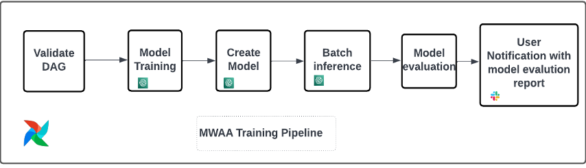
MWAA Training Pipeline

We use the following operators in the deployment pipeline (shown in the following workflow diagram):

• SageMakerModelOperator
• SageMakerEndpointConfigOperator
• SageMakerEndpointOperator

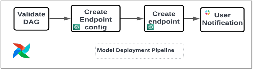
Model Deployment Pipeline

We use Slack and Amazon SNS to publish the error/success messages and evaluation results in both pipelines. Slack provides a wide range of options to customize messages, including the following:

• SnsPublishOperator – We use SnsPublishOperator to send success/failure notifications to user emails
• Slack API – We created the incoming webhook URL to get the pipeline notifications to the desired channel

CloudWatch and VMware Wavefront: Monitoring and logging

We use a CloudWatch dashboard to configure endpoint monitoring and logging. It helps visualize and keep track of various operational and model performance metrics specific to each project. On top of the auto scaling policies set up to track some of them, we continuously monitor the changes in CPU and memory usage, requests per second, response latencies, and model metrics.

CloudWatch is even integrated with a VMware Tanzu Wavefront dashboard so that it can visualize the metrics for model endpoints as well as other services at the project level.

Business benefits and what’s next

ML pipelines are very crucial to ML services and features. In this post, we discussed an end-to-end ML use case using capabilities from AWS. We built a custom pipeline using SageMaker and Amazon MWAA, which we can reuse across projects and models, and automated the ML lifecycle, which reduced the time from model training to production deployment to as little as 10 minutes.

With the shifting of the ML lifecycle burden to SageMaker, it provided optimized and scalable infrastructure for the model training and deployment. Model serving with SageMaker helped us make real-time predictions with millisecond latencies and monitoring capabilities. We used Terraform for the ease of setup and to manage infrastructure.

The next steps for this pipeline would be to enhance the model training pipeline with retraining capabilities whether it’s scheduled or based on model drift detection, support shadow deployment or A/B testing for faster and qualified model deployment, and ML lineage tracking. We also plan to evaluate Amazon SageMaker Pipelines because GitLab integration is now supported.

Lessons learned

As part of building this solution, we learned that you should generalize early, but don’t over-generalize. When we first finished the architecture design, we tried to create and enforce code templating for the model code as a best practice. However, it was so early on in the development process that the templates were either too generalized or too detailed to be reusable for future models.

After delivering the first model through the pipeline, the templates came out naturally based on the insights from our previous work. A pipeline can’t do everything from day one.

Model experimentation and productionization often have very different (or sometimes even conflicting) requirements. It is crucial to balance these requirements from the beginning as a team and prioritize accordingly.

Additionally, you might not need every feature of a service. Using essential features from a service and having a modularized design are keys to more efficient development and a flexible pipeline.

Conclusion

In this post, we showed how we built an MLOps solution using SageMaker and Amazon MWAA that automated the process of deploying models to production, with little manual intervention from data scientists. We encourage you to evaluate various AWS services like SageMaker, Amazon MWAA, Amazon S3, and Amazon ECR to build a complete MLOps solution.

*Apache, Apache Airflow, and Airflow are either registered trademarks or trademarks of the Apache Software Foundation in the United States and/or other countries.

About the Authors

 Deepak Mettem is a Senior Engineering Manager in VMware, Carbon Black Unit. He and his team work on building the streaming based applications and services that are highly available, scalable and resilient to bring customers machine learning based solutions in real-time. He and his team are also responsible for creating tools necessary for data scientists to build, train, deploy and validate their ML models in production.

Mahima Agarwal is a Machine Learning Engineer in VMware, Carbon Black Unit.
She works on designing, building, and developing the core components and architecture of the machine learning platform for the VMware CB SBU.

Vamshi Krishna Enabothala is a Sr. Applied AI Specialist Architect at AWS. He works with customers from different sectors to accelerate high-impact data, analytics, and machine learning initiatives. He is passionate about recommendation systems, NLP, and computer vision areas in AI and ML. Outside of work, Vamshi is an RC enthusiast, building RC equipment (planes, cars, and drones), and also enjoys gardening.

Sahil Thapar is an Enterprise Solutions Architect. He works with customers to help them build highly available, scalable, and resilient applications on the AWS Cloud. He is currently focused on containers and machine learning solutions.

Read More

Amazon SageMaker Ground Truth Plus is a managed data labeling service that makes it easy to label data for machine learning (ML) applications. One common use case is semantic segmentation, which is a computer vision ML technique that involves assigning class labels to individual pixels in an image. For example, in video frames captured by a moving vehicle, class labels can include vehicles, pedestrians, roads, traffic signals, buildings, or backgrounds. It provides a high-precision understanding of the locations of different objects in the image and is often used to build perception systems for autonomous vehicles or robotics. To build an ML model for semantic segmentation, it is first necessary to label a large volume of data at the pixel level. This labeling process is complex. It requires skilled labelers and significant time—some images can take up to 2 hours or more to label accurately!

In 2019, we released an ML-powered interactive labeling tool called Auto-segment for Ground Truth that allows you to quickly and easily create high-quality segmentation masks. For more information, see Auto-Segmentation Tool. This feature works by allowing you to click the top-, left-, bottom-, and right-most “extreme points” on an object. An ML model running in the background will ingest this user input and return a high-quality segmentation mask that immediately renders in the Ground Truth labeling tool. However, this feature only allows you to place four clicks. In certain cases, the ML-generated mask may inadvertently miss certain portions of an image, such as around the object boundary where edges are indistinct or where color, saturation, or shadows blend into the surroundings.

Extreme point clicking with a flexible number of corrective clicks

We now have enhanced the tool to allow extra clicks of boundary points, which provides real-time feedback to the ML model. This allows you to create a more accurate segmentation mask. In the following example, the initial segmentation result isn’t accurate because of the weak boundaries near the shadow. Importantly, this tool operates in a mode that allows for real-time feedback—it doesn’t require you to specify all points at once. Instead, you can first make four mouse clicks, which will trigger the ML model to produce a segmentation mask. Then you can inspect this mask, locate any potential inaccuracies, and subsequently place additional clicks as appropriate to “nudge” the model into the correct result.

Our previous labeling tool allowed you to place exactly four mouse clicks (red dots). The initial segmentation result (shaded red area) isn’t accurate because of the weak boundaries near the shadow (bottom-left of red mask).

With our enhanced labeling tool, the user again first makes four mouse clicks (red dots in top figure). Then you have the opportunity to inspect the resulting segmentation mask (shaded red area in top figure). You can make additional mouse clicks (green dots in bottom figure) to cause the model to refine the mask (shaded red area in bottom figure).

Compared with the original version of the tool, the enhanced version provides an improved result when objects are deformable, non-convex, and vary in shape and appearance.

We simulated the performance of this improved tool on sample data by first running the baseline tool (with only four extreme clicks) to generate a segmentation mask and evaluated its mean Intersection over Union (mIoU), a common measure of accuracy for segmentation masks. Then we applied simulated corrective clicks and evaluated the improvement in mIoU after each simulated click. The following table summarizes these results. The first row shows the mIoU, and the second row shows the error (which is given by 100% minus the mIoU). With only five additional mouse clicks, we can reduce the error by 9% for this task!

Integration with Ground Truth and performance profiling

To integrate this model with Ground Truth, we follow a standard architecture pattern as shown in the following diagram. First, we build the ML model into a Docker image and deploy it to Amazon Elastic Container Registry (Amazon ECR), a fully managed Docker container registry that makes it easy to store, share, and deploy container images. Using the SageMaker Inference Toolkit in building the Docker image allows us to easily use best practices for model serving and achieve low-latency inference. We then create an Amazon SageMaker real-time endpoint to host the model. We introduce an AWS Lambda function as a proxy in front of the SageMaker endpoint to offer various types of data transformation. Finally, we use Amazon API Gateway as a way of integrating with our front end, the Ground Truth labeling application, to provide secure authentication to our backend.

You can follow this generic pattern for your own use cases for purpose-built ML tools and to integrate them with custom Ground Truth task UIs. For more information, refer to Build a custom data labeling workflow with Amazon SageMaker Ground Truth.

After provisioning this architecture and deploying our model using the AWS Cloud Development Kit (AWS CDK), we evaluated the latency characteristics of our model with different SageMaker instance types. This is very straightforward to do because we use SageMaker real-time inference endpoints to serve our model. SageMaker real-time inference endpoints integrate seamlessly with Amazon CloudWatch and emit such metrics as memory utilization and model latency with no required setup (see SageMaker Endpoint Invocation Metrics for more details).

In the following figure, we show the ModelLatency metric natively emitted by SageMaker real-time inference endpoints. We can easily use various metric math functions in CloudWatch to show latency percentiles, such as p50 or p90 latency.

The following table summarizes these results for our enhanced extreme clicking tool for semantic segmentation for three instance types: p2.xlarge, p3.2xlarge, and g4dn.xlarge. Although the p3.2xlarge instance provides the lowest latency, the g4dn.xlarge instance provides the best cost-to-performance ratio. The g4dn.xlarge instance is only 8% slower (35 milliseconds) than the p3.2xlarge instance, but it is 81% less expensive on an hourly basis than the p3.2xlarge (see Amazon SageMaker Pricing for more details on SageMaker instance types and pricing).

Conclusion

In this post, we introduced an extension to the Ground Truth auto segment feature for semantic segmentation annotation tasks. Whereas the original version of the tool allows you to make exactly four mouse clicks, which triggers a model to provide a high-quality segmentation mask, the extension enables you to make corrective clicks and thereby update and guide the ML model to make better predictions. We also presented a basic architectural pattern that you can use to deploy and integrate interactive tools into Ground Truth labeling UIs. Finally, we summarized the model latency, and showed how the use of SageMaker real-time inference endpoints makes it easy to monitor model performance.

To learn more about how this tool can reduce labeling cost and increase accuracy, visit Amazon SageMaker Data Labeling to start a consultation today.

About the authors

Jonathan Buck is a Software Engineer at Amazon Web Services working at the intersection of machine learning and distributed systems. His work involves productionizing machine learning models and developing novel software applications powered by machine learning to put the latest capabilities in the hands of customers.

Li Erran Li is the applied science manager at humain-in-the-loop services, AWS AI, Amazon. His research interests are 3D deep learning, and vision and language representation learning. Previously he was a senior scientist at Alexa AI, the head of machine learning at Scale AI and the chief scientist at Pony.ai. Before that, he was with the perception team at Uber ATG and the machine learning platform team at Uber working on machine learning for autonomous driving, machine learning systems and strategic initiatives of AI. He started his career at Bell Labs and was adjunct professor at Columbia University. He co-taught tutorials at ICML’17 and ICCV’19, and co-organized several workshops at NeurIPS, ICML, CVPR, ICCV on machine learning for autonomous driving, 3D vision and robotics, machine learning systems and adversarial machine learning. He has a PhD in computer science at Cornell University. He is an ACM Fellow and IEEE Fellow.

Read More

Amazon SageMaker Data Wrangler reduces the time it takes to aggregate and prepare data for machine learning (ML) from weeks to minutes in Amazon SageMaker Studio. Data Wrangler enables you to access data from a wide variety of popular sources (Amazon S3, Amazon Athena, Amazon Redshift, Amazon EMR and Snowflake) and over 40 other third-party sources. Starting today, you can connect to Amazon EMR Hive as a big data query engine to bring in large datasets for ML.

Aggregating and preparing large amounts of data is a critical part of ML workflow. Data scientists and data engineers use Apache Spark, Apache Hive, and Presto running on Amazon EMR for large-scale data processing. This blog post will go through how data professionals may use SageMaker Data Wrangler’s visual interface to locate and connect to existing Amazon EMR clusters with Hive endpoints. To get ready for modeling or reporting, they can visually analyze the database, tables, schema, and author Hive queries to create the ML dataset. Then, they can quickly profile data using Data Wrangler visual interface to evaluate data quality, spot anomalies and missing or incorrect data, and get advice on how to deal with these problems. They can leverage more popular and ML-powered built-in analyses and 300+ built-in transformations supported by Spark to analyze, clean, and engineer features without writing a single line of code. Finally, they can also train and deploy models with SageMaker Autopilot, schedule jobs, or operationalize data preparation in a SageMaker Pipeline from Data Wrangler’s visual interface.

Solution overview

With SageMaker Studio setups, data professionals can quickly identify and connect to existing EMR clusters. In addition, data professionals can discover EMR clusters from SageMaker Studio using predefined templates on demand in just a few clicks. Customers can use SageMaker Studio universal notebook and write code in Apache Spark, Hive, Presto or PySpark to perform data preparation at scale. However, not all data professionals are familiar with writing Spark code to prepare data because there is a steep learning curve involved. They can now quickly and simply connect to Amazon EMR without writing a single line of code, thanks to Amazon EMR being a data source for Amazon SageMaker Data Wrangler.

The following diagram represents the different components used in this solution.

We demonstrate two authentication options that can be used to establish a connection to the EMR cluster. For each option, we deploy a unique stack of AWS CloudFormation templates.

The CloudFormation template performs the following actions when each option is selected:

• Creates a Studio Domain in VPC-only mode, along with a user profile named studio-user.
• Creates building blocks, including the VPC, endpoints, subnets, security groups, EMR cluster, and other required resources to successfully run the examples.
• For the EMR cluster, connects the AWS Glue Data Catalog as metastore for EMR Hive and Presto, creates a Hive table in EMR, and fills it with data from a US airport dataset.
• For the LDAP CloudFormation template, creates an Amazon Elastic Compute Cloud (Amazon EC2) instance to host the LDAP server to authenticate the Hive and Presto LDAP user.

Option 1: Lightweight Access Directory Protocol 

For the LDAP authentication CloudFormation template, we provision an Amazon EC2 instance with an LDAP server and configure the EMR cluster to use this server for authentication. This is TLS enabled.

Option 2: No-Auth

In the No-Auth authentication CloudFormation template, we use a standard EMR cluster with no authentication enabled.

Deploy the resources with AWS CloudFormation

Complete the following steps to deploy the environment:

1. Sign in to the AWS Management Console as an AWS Identity and Access Management (IAM) user, preferably an admin user.
2. Choose Launch Stack to launch the CloudFormation template for the appropriate authentication scenario. Make sure the Region used to deploy the CloudFormation stack has no existing Studio Domain. If you already have a Studio Domain in a Region, you may choose a different Region.
   

   LDAP
   No Auth

3. Choose Next.
4. For Stack name, enter a name for the stack (for example, dw-emr-hive-blog).
5. Leave the other values as default.
6. To continue, choose Next from the stack details page and stack options.
   The LDAP stack uses the following credentials.
   •  username: david
   •  password:  welcome123
7. On the review page, select the check box to confirm that AWS CloudFormation might create resources.
8. Choose Create stack. Wait until the status of the stack changes from CREATE_IN_PROGRESS to CREATE_COMPLETE. The process usually takes 10–15 minutes.

Set up the Amazon EMR as a data source in Data Wrangler

In this section, we cover connecting to the existing Amazon EMR cluster created through the CloudFormation template as a data source in Data Wrangler.

Create a new data flow

To create your data flow, complete the following steps:

1. On the SageMaker console, click Domains, then click on StudioDomain created by running above CloudFormation template.
2. Select studio-user user profile and launch Studio.
   
3. Choose Open studio.
4. In the Studio Home console, choose Import & prepare data visually. Alternatively, on the File dropdown, choose New, then choose Data Wrangler Flow.
5. Creating a new flow can take a few minutes. After the flow has been created, you see the Import data page.
   
6. Add Amazon EMR as a data source in Data Wrangler. On the Add data source menu, choose Amazon EMR.
   

You can browse all the EMR clusters that your Studio execution role has permissions to see. You have two options to connect to a cluster; one is through interactive UI, and the other is to first create a secret using AWS Secrets Manager with JDBC URL, including EMR cluster information, and then provide the stored AWS secret ARN in the UI to connect to Hive. In this blog, we follow the first option.

7. Select one of the following clusters that you want to use. Click on Next, and select endpoints.
   
8. Select Hive, connect to Amazon EMR, create a name to identify your connection, and click Next.
   
9. Select authentication type, either Lightweight Directory Access Protocol (LDAP) or No authentication.

For Lightweight Directory Access Protocol (LDAP), select the option and click Next, login to cluster, then provide username and password to be authenticated and click Connect.

For No Authentication, you will be connected to EMR Hive without providing user credentials within VPC. Enter Data Wrangler’s SQL explorer page for EMR.

10. Once connected, you can interactively view a database tree and table preview or schema. You can also query, explore, and visualize data from EMR. For preview, you would see a limit of 100 records by default. Once you provide a SQL statement in the query editor box and click the Run button, the query will be executed on EMR’s Hive engine to preview the data.
    

The Cancel query button allows ongoing queries to be canceled if they are taking an unusually long time.

11. The last step is to import. Once you are ready with the queried data, you have options to update the sampling settings for the data selection according to the sampling type (FirstK, Random, or Stratified) and sampling size for importing data into Data Wrangler.

Click Import. The prepare page will be loaded, allowing you to add various transformations and essential analysis to the dataset.

12. Navigate to Data flow from the top screen and add more steps to the flow as needed for transformations and analysis. You can run a data insight report to identify data quality issues and get recommendations to fix those issues. Let’s look at some example transforms.
13. In the Data flow view, you should see that we are using EMR as a data source using the Hive connector.
    
14. Let’s click on the + button to the right of Data types and select Add transform. When you do that, you will go back to the Data view.
    

Let’s explore the data. We see that it has multiple features such as  iata_code, airport, city, state, country, latitude, and longitude. We can see that the entire dataset is based in one country, which is the US, and there are missing values in latitude and longitude. Missing data can cause bias in the estimation of parameters, and it can reduce the representativeness of the samples, so we need to perform some imputation and handle missing values in our dataset.

15. Let’s click on the Add Step button on the navigation bar to the right. Select Handle missing. The configurations can be seen in the following screenshots.

Under Transform, select Impute. Select the Column type as Numeric and Input column names latitude and longitude. We will be imputing the missing values using an approximate median value.

First click on Preview to view the missing value and then click on update to add the transform.

16. Let us now look at another example transform. When building an ML model, columns are removed if they are redundant or don’t help your model. The most common way to remove a column is to drop it. In our dataset, the feature country can be dropped since the dataset is specifically for US airport data. To manage columns, click on the Add step button on the navigation bar to the right and select Manage columns. The configurations can be seen in the following screenshots. Under Transform, select Drop column, and under Columns to drop, select country.
    
    
17. Click on Preview and then Update to drop the column.
    
18. Feature Store is a repository to store, share, and manage features for ML models. Let’s click on the + button to the right of Drop column. Select Export to and choose SageMaker Feature Store (via Jupyter notebook).
    
19. By selecting SageMaker Feature Store as the destination, you can save the features into an existing feature group or create a new one.
    
    

We have now created features with Data Wrangler and easily stored those features in Feature Store. We showed an example workflow for feature engineering in the Data Wrangler UI. Then we saved those features into Feature Store directly from Data Wrangler by creating a new feature group. Finally, we ran a processing job to ingest those features into Feature Store. Data Wrangler and Feature Store together helped us build automatic and repeatable processes to streamline our data preparation tasks with minimum coding required. Data Wrangler also provides us flexibility to automate the same data preparation flow using scheduled jobs. We can also automatically train and deploy models using SageMaker Autopilot from Data Wrangler’s visual interface, or create training or feature engineering pipeline with SageMaker Pipelines (via Jupyter Notebook) and deploy to the inference endpoint with SageMaker inference pipeline (via Jupyter Notebook).

Clean up

If your work with Data Wrangler is complete, the following steps will help you delete the resources created to avoid incurring additional fees.

1. Shut down SageMaker Studio.

From within SageMaker Studio, close all the tabs, then select File then Shut Down. Once prompted select Shutdown All.

Shutdown might take a few minutes based on the instance type. Make sure all the apps associated with the user profile got deleted. If they were not deleted, manually delete the app associated under user profile.

2. Empty any S3 buckets that were created from CloudFormation launch.

Open the Amazon S3 page by searching for S3 in the AWS console search. Empty any S3 buckets that were created when provisioning clusters. The bucket would be of format dw-emr-hive-blog-.

3. Delete the SageMaker Studio EFS.

Open the EFS page by searching for EFS in the AWS console search.

Locate the filesystem that was created by SageMaker. You can confirm this by clicking on the File system ID and confirming the tag ManagedByAmazonSageMakerResource on the Tags tab.

4. Delete the CloudFormation stacks. Open CloudFormation by searching for and opening the CloudFormation service from the AWS console.

Select the template starting with dw- as shown in the following screen and delete the stack as shown by clicking on the Delete button.

This is expected and we will come back to this and clean it up in the subsequent steps.

5. Delete the VPC after the CloudFormation stack fails to complete. First open VPC from the AWS console.
6. Next, identify the VPC that was created by the SageMaker Studio CloudFormation, titled dw-emr-, and then follow the prompts to delete the VPC.
   
7. Delete the CloudFormation stack.

Return to CloudFormation and retry the stack deletion for dw-emr-hive-blog.

Complete! All the resources provisioned by the CloudFormation template described in this blog post will now be removed from your account.

Conclusion

In this post, we went over how to set up Amazon EMR as a data source in Data Wrangler, how to transform and analyze a dataset, and how to export the results to a data flow for use in a Jupyter notebook. After visualizing our dataset using Data Wrangler’s built-in analytical features, we further enhanced our data flow. The fact that we created a data preparation pipeline without writing a single line of code is significant.

To get started with Data Wrangler, see Prepare ML Data with Amazon SageMaker Data Wrangler and see the latest information on the Data Wrangler product page  and AWS technical documents.

About the Authors

Ajjay Govindaram is a Senior Solutions Architect at AWS. He works with strategic customers who are using AI/ML to solve complex business problems. His experience lies in providing technical direction as well as design assistance for modest to large-scale AI/ML application deployments. His knowledge ranges from application architecture to big data, analytics, and machine learning. He enjoys listening to music while resting, experiencing the outdoors, and spending time with his loved ones.

Isha Dua is a Senior Solutions Architect based in the San Francisco Bay Area. She helps AWS enterprise customers grow by understanding their goals and challenges, and guides them on how they can architect their applications in a cloud-native manner while ensuring resilience and scalability. She’s passionate about machine learning technologies and environmental sustainability.

Varun Mehta is a Solutions Architect at AWS. He is passionate about helping customers build Enterprise-Scale Well-Architected solutions on the AWS Cloud. He works with strategic customers who are using AI/ML to solve complex business problems.

Read More

In this two-part series, we demonstrate how to label and train models for 3D object detection tasks. In part 1, we discuss the dataset we’re using, as well as any preprocessing steps, to understand and label data. In part 2, we walk through how to train a model on your dataset and deploy it to production.

LiDAR (light detection and ranging) is a method for determining ranges by targeting an object or surface with a laser and measuring the time for the reflected light to return to the receiver. Autonomous vehicle companies typically use LiDAR sensors to generate a 3D understanding of the environment around their vehicles.

As LiDAR sensors become more accessible and cost-effective, customers are increasingly using point cloud data in new spaces like robotics, signal mapping, and augmented reality. Some new mobile devices even include LiDAR sensors. The growing availability of LiDAR sensors has increased interest in point cloud data for machine learning (ML) tasks, like 3D object detection and tracking, 3D segmentation, 3D object synthesis and reconstruction, and using 3D data to validate 2D depth estimation.

In this series, we show you how to train an object detection model that runs on point cloud data to predict the location of vehicles in a 3D scene. This post, we focus specifically on labeling LiDAR data. Standard LiDAR sensor output is a sequence of 3D point cloud frames, with a typical capture rate of 10 frames per second. To label this sensor output you need a labeling tool that can handle 3D data. Amazon SageMaker Ground Truth makes it easy to label objects in a single 3D frame or across a sequence of 3D point cloud frames for building ML training datasets. Ground Truth also supports sensor fusion of camera and LiDAR data with up to eight video camera inputs.

Data is essential to any ML project. 3D data in particular can be difficult to source, visualize, and label. We use the A2D2 dataset in this post and walk you through the steps to visualize and label it.

A2D2 contains 40,000 frames with semantic segmentation and point cloud labels, including 12,499 frames with 3D bounding box labels. Since we are focusing on object detection, we’re interested in the 12,499 frames with 3D bounding box labels. These annotations include 14 classes relevant to driving like car, pedestrian, truck, bus, etc.

The following table shows the complete class list:

We will train our detector to specifically detect cars since that’s the most common class in our dataset (32616 of the 42816 total objects in the dataset are labeled as cars).

Solution overview

In this series, we cover how to visualize and label your data with Amazon SageMaker Ground Truth and demonstrate how to use this data in an Amazon SageMaker training job to create an object detection model, deployed to an Amazon SageMaker Endpoint. In particular, we’ll use an Amazon SageMaker notebook to operate the solution and launch any labeling or training jobs.

The following diagram depicts the overall flow of sensor data from labeling to training to deployment:

You’ll learn how to train and deploy a real-time 3D object detection model with Amazon SageMaker Ground Truth with the following steps:

1. Download and visualize a point cloud dataset
2. Prep data to be labeled with the Amazon SageMaker Ground Truth point cloud tool
3. Launch a distributed Amazon SageMaker Ground Truth training job with MMDetection3D
4. Evaluate your training job results and profiling your resource utilization with Amazon SageMaker Debugger
5. Deploy an asynchronous SageMaker endpoint
6. Call the endpoint and visualizing 3D object predictions

AWS services used to Implement this solution

• Amazon SageMaker Ground Truth
• Amazon SageMaker Training
• Amazon SageMaker Inference
• Amazon SageMaker Notebooks
• Amazon FSx for Lustre
• Amazon Simple Storage Service (Amazon S3)

Prerequisites

• An AWS account.
• Familiarity with Amazon SageMaker Ground Truth and AWS CloudFormation
• An Amazon SageMaker workforce. For this demonstration, we use a private workforce. You can create a workforce through the SageMaker console.

The following diagram demonstrates how to create a private workforce. For written, step-by-step instructions, see Create an Amazon Cognito Workforce Using the Labeling Workforces Page.

Launching the AWS CloudFormation stack

Now that you’ve seen the structure of the solution, you deploy it into your account so you can run an example workflow. All the deployment steps related to the labeling pipeline are managed by AWS CloudFormation. This means AWS Cloudformation creates your notebook instance as well as any roles or Amazon S3 Buckets to support running the solution.

You can launch the stack in AWS Region us-east-1 on the AWS CloudFormation console using the Launch Stack
button. To launch the stack in a different Region, use the instructions found in the README of the GitHub repository.

This takes approximately 20 minutes to create all the resources. You can monitor the progress from the AWS CloudFormation user interface (UI).

Once your CloudFormation template is done running go back to the AWS Console.

Opening the Notebook

Amazon SageMaker Notebook Instances are ML compute instances that run on the Jupyter Notebook App. Amazon SageMaker manages the creation of instances and related resources. Use Jupyter notebooks in your notebook instance to prepare and process data, write code to train models, deploy models to Amazon SageMaker hosting, and test or validate your models.

Follow the next steps to access the Amazon SageMaker Notebook environment:

1. Under services search for Amazon SageMaker.
   
2. Under Notebook, select Notebook instances.
   
3. A Notebook instance should be provisioned. Select Open JupyterLab, which is located on the right side of the pre-provisioned Notebook instance under Actions.
   
4. You’ll see an icon like this as the page loads:
   
5. You’ll be redirected to a new browser tab that looks like the following diagram:
   
6. Once you are in the Amazon SageMaker Notebook Instance Launcher UI. From the left sidebar, select the Git icon as shown in the following diagram.
   
7. Select Clone a Repository option.
   
8. Enter GitHub URL(https://github.com/aws-samples/end-2-end-3d-ml) in the pop‑up window and choose clone.
   
9. Select File Browser to see the GitHub folder.
   
10. Open the notebook titled 1_visualization.ipynb.

Operating the Notebook

Overview

The first few cells of the notebook in the section titled Downloaded Files walks through how to download the dataset and inspect the files within it. After the cells are executed, it takes a few minutes for the data to finish downloading.

Once downloaded, you can review the file structure of A2D2, which is a list of scenes or drives. A scene is a short recording of sensor data from our vehicle. A2D2 provides 18 of these scenes for us to train on, which are all identified by unique dates. Each scene contains 2D camera data, 2D labels, 3D cuboid annotations, and 3D point clouds.

You can view the file structure for the A2D2 dataset with the following:

├── 20180807_145028
├── 20180810_142822
│   ├── camera
│   │   ├── cam_front_center
│   │   │   ├── 20180807145028_lidar_frontcenter_000000091.png
│   │   │   ├── 20180807145028_lidar_frontcenter_000000091.json
│   │   │   ├── 20180807145028_lidar_frontcenter_000000380.png
│   │   │   ├── 20180807145028_lidar_frontcenter_000000380.json
│   │   │   ├── ...
│   ├── label
│   │   ├── cam_front_center
│   │   │   ├── 20180807145028_lidar_frontcenter_000000091.png
│   │   │   ├── 20180807145028_lidar_frontcenter_000000380.png
│   │   │   ├── ...
│   ├── label3D
│   │   ├── cam_front_center
│   │   │   ├── 20180807145028_lidar_frontcenter_000000091.json
│   │   │   ├── 20180807145028_lidar_frontcenter_000000380.json
│   │   │   ├── ...
│   ├── lidar
│   │   ├── cam_front_center
│   │   │   ├── 20180807145028_lidar_frontcenter_000000091.npz
│   │   │   ├── 20180807145028_lidar_frontcenter_000000380.npz
│   │   │   ├── ...

A2D2 sensor setup

The next section walks through reading some of this point cloud data to make sure we’re interpreting it correctly and can visualize it in the notebook before trying to convert it into a format ready for data labeling.

For any kind of autonomous driving setup where we have 2D and 3D sensor data, capturing sensor calibration data is essential. In addition to the raw data, we also downloaded cams_lidar.json. This file contains the translation and orientation of each sensor relative to the vehicle’s coordinate frame, this can also be referred to as the sensor’s pose, or location in space. This is important for converting points from a sensor’s coordinate frame to the vehicle’s coordinate frame. In other words, it’s important for visualizing the 2D and 3D sensors as the vehicle drives. The vehicle’s coordinate frame is defined as a static point in the center of the vehicle, with the x-axis in the direction of the forward movement of the vehicle, the y-axis denoting left and right with left being positive, and the z-axis pointing through the roof of the vehicle. A point (X,Y,Z) of (5,2,1) means this point is 5 meters ahead of our vehicle, 2 meters to the left, and 1 meter above our vehicle. Having these calibrations also allows us to project 3D points onto our 2D image, which is especially helpful for point cloud labeling tasks.

To see the sensor setup on the vehicle, check the following diagram.

The point cloud data we are training on is specifically aligned with the front facing camera or cam front-center:

This matches our visualization of camera sensors in 3D:

This portion of the notebook walks through validating that the A2D2 dataset matches our expectations about sensor positions, and that we’re able to align data from the point cloud sensors into the camera frame. Feel free to run all cells through the one titled Projection from 3D to 2D to see your point cloud data overlay on the following camera image.

Conversion to Amazon SageMaker Ground Truth

After visualizing our data in our notebook, we can confidently convert our point clouds into Amazon SageMaker Ground Truth’s 3D format to verify and adjust our labels. This section walks through converting from A2D2’s data format into an Amazon SageMaker Ground Truth sequence file, with the input format used by the object tracking modality.

The sequence file format includes the point cloud formats, the images associated with each point cloud, and all sensor position and orientation data required to align images with point clouds. These conversions are done using the sensor information read from the previous section. The following example is a sequence file format from Amazon SageMaker Ground Truth, which describes a sequence with only a single timestep.

The point cloud for this timestep is located at s3://sagemaker-us-east-1-322552456788/a2d2_smgt/20180807_145028_out/20180807145028_lidar_frontcenter_000000091.txt and has a format of <x coordinate> <y coordinate> <z coordinate>.

Associated with the point cloud, is a single camera image located at s3://sagemaker-us-east-1-322552456788/a2d2_smgt/20180807_145028_out/undistort_20180807145028_camera_frontcenter_000000091.png. Notice that we take the sequence file that defines all camera parameters to allow projection from the point cloud to the camera and back.

 {
 "seq-no": 1,
  "prefix": "s3://sagemaker-us-east-1-322552456788/a2d2_smgt/20180807_145028_out/",
  "number-of-frames": 1,
  "frames": [
    {
      "frame-no": 0,
      "unix-timestamp": 0.091,
      "frame": "20180807145028_lidar_frontcenter_000000091.txt",
      "format": "text/xyz",
      "ego-vehicle-pose": {
        "position": {
          "x": 0,
          "y": 0,
          "z": 0},
        "heading": {
          "qw": 1,
          "qx": 0,
          "qy": 0,
          "qz": 0}},
      "images": [
        {
          "image-path": "undistort_20180807145028_camera_frontcenter_000000091.png",
          "unix-timestamp": 0.091,
          "fx": 1687.3369140625,
          "fy": 1783.428466796875,
          "cx": 965.4341405582381,
          "cy": 684.4193604186803,
          "position": {
            "x": 1.711045726422736,
            "y": -5.735179668849011e-09,
            "z": 0.9431449279047172},
          "heading": {
            "qw": -0.4981871970275329,
            "qx": 0.5123971466375787,
            "qy": -0.4897950939891415,
            "qz": 0.4993590359047143},
          "camera-model": "pinhole"}]},
    }
  ]
}

Conversion to this input format requires us to write a conversion from A2D2’s data format to data formats supported by Amazon SageMaker Ground Truth. This is the same process anyone must undergo when bringing their own data for labeling. We’ll walk through how this conversion works, step-by-step. If following along in the notebook, look at the function named a2d2_scene_to_smgt_sequence_and_seq_label.

Point cloud conversion

The first step is to convert the data from a compressed Numpy-formatted file (NPZ), which was generated with the numpy.savez method, to an accepted raw 3D format for Amazon SageMaker Ground Truth. Specifically, we generate a file with one row per point. Each 3D point is defined by three floating point X, Y, and Z coordinates. When we specify our format in the sequence file, we use the string text/xyz to represent this format. Amazon SageMaker Ground Truth also supports adding intensity values or Red Green Blue (RGB) points.

A2D2’s NPZ files contain multiple Numpy arrays, each with its own name. To perform a conversion, we load the NPZ file using Numpy’s load method, access the array called points (i.e., an Nx3 array, where N is the number of points in the point cloud), and save as text to a new file using Numpy’s savetxt method.

# input.npz is an A2D2 PointCloud file
lidar_frame_contents = np.load("a2d2_input.npz")
points = lidar_frame_contents["points"]
# output.txt is a text/xyz formatted SMGT file
np.savetxt("output.txt", points)

Image preprocessing

Next, we prepare our image files. A2D2 provides PNG images, and Amazon SageMaker Ground Truth supports PNG images; however, these images are distorted. Distortion often occurs because the image-taking lens is not aligned parallel to the imaging plane, which makes some areas in the image look closer than expected. This distortion describes the difference between a physical camera and an idealized pinhole camera model. If distortion isn’t taken into account, then Amazon SageMaker Ground Truth won’t be able to render our 3D points on top of the camera views, which makes it more challenging to perform labeling. For a tutorial on camera calibration, look at this documentation from OpenCV.

While Amazon SageMaker Ground Truth supports distortion coefficients in its input file, you can also perform preprocessing before the labeling job. Since A2D2 provides helper code to perform undistortion, we apply it to the image, and leave the fields related to distortion out of our sequence file. Note that the distortion related fields include k1, k2, k3, k4, p1, p2, and skew.

from a2d2_helpers import undistort_image
# distorted_input.png comes from the A2D2 dataset
image_frame = cv2.imread("distorted_input.png")
# we undistort the front_center camera, and pass the cams_lidars dictionary
# which contains all camera distortion coefficients.
undistorted_image = undistort_image(image_frame, "front_center", cams_lidars)
# undistorted_output.png goes into SMGT's output path
cv2.imwrite("undistorted_output.png", undistorted_image)

Camera position, orientation, and projection conversion

Beyond the raw data files required for labeling, the sequence file also requires camera position and orientation information to perform the projection of 3D points into the 2D camera views. We need to know where the camera is looking in 3D space to figure out how 3D cuboid labels and 3D points should be rendered on top of our images.

Because we’ve loaded our sensor positions into a common transform manager in the A2D2 sensor setup section, we can easily query the transform manager for the information we want. In our case, we treat the vehicle position as (0, 0, 0) in each frame because we don’t have position information of the sensor provided by A2D2’s object detection dataset. So relative to our vehicle, the camera’s orientation and position is described by the following code:

# The format of pq = [x, y, z, qw, qx, qy, qz] where (x, y, z) refer to object
# position while the remaining (qw, qx, qy, qz) correspond to camera orientation.
pq = transform_manager.get_transform("cam_front_center_ext", "vehicle")
# pq can then be extracted into SMGT's sequence file format as below:
{
...
"position": {"x": pq[0],"y": pq[1],"z": pq[2]},
"heading": {"qw": pq[3],"qx": pq[4],"qy": pq[5],"qz": pq[6],}
}

Now that position and orientation are converted, we also need to supply values for fx, fy, cx, and cy, all parameters for each camera in the sequence file format.

These parameters refer to values in the camera matrix. While the position and orientation describe which way a camera is facing, the camera matrix describes the field of the view of the camera and exactly how a 3D point relative to the camera gets converted to a 2D pixel location in an image.

A2D2 provides a camera matrix. A reference camera matrix is shown in the following code, along with how our notebook indexes this matrix to get the appropriate fields.

# [[fx,  0, cx]
#  [ 0, fy, cy]
#  [ 0,  0,  1]]
{
...
"fx": camera_matrix[0, 0],
"fy": camera_matrix[1, 1],
"cx": camera_matrix[0, 2],
"cy": camera_matrix[1, 2]
}

With all of the fields parsed from A2D2’s format, we can save the sequence file and use it in an Amazon SageMaker Ground Truth input manifest file to start a labeling job. This labeling job allows us to create 3D bounding box labels to use downstream for 3D model training.

Run all cells until the end of the notebook, and ensure you replace the workteam ARN with the Amazon SageMaker Ground Truth workteam ARN you created a prerequisite. After about 10 minutes of labeling job creation time, you should be able to login to the worker portal and use the labeling user interface to visualize your scene.

Clean up

Delete the AWS CloudFormation stack you deployed using the Launch Stack button named ThreeD in the AWS CloudFormation console to remove all resources used in this post, including any running instances.

Estimated costs

The approximate cost is $5 for 2 hours.

Conclusion

In this post, we demonstrated how to take 3D data and convert it into a form ready for labeling in Amazon SageMaker Ground Truth. With these steps, you can label your own 3D data for training object detection models. In the next post in this series, we’ll show you how to take A2D2 and train an object detector model on the labels already in the dataset.

Happy Building!

About the Authors

Isaac Privitera is a Senior Data Scientist at the Amazon Machine Learning Solutions Lab, where he develops bespoke machine learning and deep learning solutions to address customers’ business problems. He works primarily in the computer vision space, focusing on enabling AWS customers with distributed training and active learning.

 Vidya Sagar Ravipati is Manager at the Amazon Machine Learning Solutions Lab, where he leverages his vast experience in large-scale distributed systems and his passion for machine learning to help AWS customers across different industry verticals accelerate their AI and cloud adoption. Previously, he was a Machine Learning Engineer in Connectivity Services at Amazon who helped to build personalization and predictive maintenance platforms.

Jeremy Feltracco is a Software Development Engineer with th Amazon Machine Learning Solutions Lab at Amazon Web Services. He uses his background in computer vision, robotics, and machine learning to help AWS customers accelerate their AI adoption.

Read More

Online fraud has a widespread impact on businesses and requires an effective end-to-end strategy to detect and prevent new account fraud and account takeovers, and stop suspicious payment transactions. Detecting fraud closer to the time of fraud occurrence is key to the success of a fraud detection and prevention system. The system should be able to detect fraud as effectively as possible also alert the end-user as quickly as possible. The user can then choose to take action to prevent further abuse.

In this post, we show a serverless approach to detect online transaction fraud in near-real time. We show how you can apply this approach to various data streaming and event-driven architectures, depending on the desired outcome and actions to take to prevent fraud (such as alert the user about the fraud or flag the transaction for additional review).

This post implements three architectures:

• Streaming data inspection and fraud detection/prevention – Using Amazon Kinesis Data Streams, AWS Lambda, AWS Step Functions, and Amazon Fraud Detector
• Streaming data enrichment for fraud detection/prevention – Using Amazon Kinesis Data Firehose, AWS Lambda, and Amazon Fraud Detector
• Event data inspection and fraud detection/prevention – Using Amazon EventBridge, AWS Step Functions, and Amazon Fraud Detector

To detect fraudulent transactions, we use Amazon Fraud Detector, a fully managed service enabling you to identify potentially fraudulent activities and catch more online fraud faster. To build an Amazon Fraud Detector model based on past data, refer to Detect online transaction fraud with new Amazon Fraud Detector features. You can also use Amazon SageMaker to train a proprietary fraud detection model. For more information, refer to Train fraudulent payment detection with Amazon SageMaker.

Streaming data inspection and fraud detection/prevention

This architecture uses Lambda and Step Functions to enable real-time Kinesis data stream data inspection and fraud detection and prevention using Amazon Fraud Detector. The same architecture applies if you use Amazon Managed Streaming for Apache Kafka (Amazon MSK) as a data streaming service. This pattern can be useful for real-time fraud detection, notification, and potential prevention. Example use cases for this could be payment processing or high-volume account creation. The following diagram illustrates the solution architecture.

The flow of the process in this implementation is as follows:

1. We ingest the financial transactions into the Kinesis data stream. The source of the data could be a system that generates these transactions—for example, ecommerce or banking.
2. The Lambda function receives the transactions in batches.
3. The Lambda function starts the Step Functions workflow for the batch.
4. For each transaction, the workflow performs the following actions:
   1. Persist the transaction in an Amazon DynamoDB table.
   2. Call the Amazon Fraud Detector API using the GetEventPrediction action. The API returns one of the following results: approve, block, or investigate.
   3. Update the transaction in the DynamoDB table with fraud prediction results.
   4. Based on the results, perform one of the following actions:
      1. Send a notification using Amazon Simple Notification Service (Amazon SNS) in case of a block or investigate response from Amazon Fraud Detector.
      2. Process the transaction further in case of an approve response.

This approach allows you to react to the potentially fraudulent transactions in real time as you store each transaction in a database and inspect it before processing further. In actual implementation, you may replace the notification step for additional review with an action that is specific to your business process—for example, inspect the transaction using some other fraud detection model, or conduct a manual review.

Streaming data enrichment for fraud detection/prevention

Sometimes, you may need to flag potentially fraudulent data but still process it; for example, when you’re storing the transactions for further analytics and collecting more data for constantly tuning the fraud detection model. An example use case is claims processing. During claims processing, you collect all the claims documents and then run them through a fraud detection system. A decision to process or reject a claim is then made—not necessarily in real time. In such cases, streaming data enrichment may fit your use case better.

This architecture uses Lambda to enable real-time Kinesis Data Firehose data enrichment using Amazon Fraud Detector and Kinesis Data Firehose data transformation.

This approach doesn’t implement fraud prevention steps. We deliver enriched data to an Amazon Simple Storage Service (Amazon S3) bucket. Downstream services that consume the data can use the fraud detection results in their business logics and act accordingly. The following diagram illustrates this architecture.

The flow of the process in this implementation is as follows:

1. We ingest the financial transactions into Kinesis Data Firehose. The source of the data could be a system that generates these transactions, such as ecommerce or banking.
2. A Lambda function receives the transactions in batches and enriches them. For each transaction in the batch, the function performs the following actions:
   1. Call the Amazon Fraud Detector API using the GetEventPrediction action. The API returns one of three results: approve, block or investigate.
   2. Update transaction data by adding fraud detection results as metadata.
   3. Return the batch of the updated transactions to the Kinesis Data Firehose delivery stream.
3. Kinesis Data Firehose delivers data to the destination (in our case, the S3 bucket).

As a result, we have data in the S3 bucket that includes not only original data but also the Amazon Fraud Detector response as metadata for each of the transactions. You can use this metadata in your data analytics solutions, machine learning model training tasks, or visualizations and dashboards that consume transaction data.

Event data inspection and fraud detection/prevention

Not all data comes into your system as a stream. However, in cases of event-driven architectures, you still can follow a similar approach.

This architecture uses Step Functions to enable real-time EventBridge event inspection and fraud detection/prevention using Amazon Fraud Detector. It doesn’t stop processing of the potentially fraudulent transaction, rather it flags the transaction for an additional review. We publish enriched transactions to an event bus that differs from the one that raw event data is being published to. This way, consumers of the data can be sure that all events include fraud detection results as metadata. The consumers can then inspect the metadata and apply their own rules based on the metadata. For example, in an event-driven ecommerce application, a consumer can choose to not process the order if this transaction is predicted to be fraudulent. This architecture pattern can also be useful for detecting and preventing fraud in new account creation or during account profile changes (like changing your address, phone number, or credit card on file in your account profile). The following diagram illustrates the solution architecture.

The flow of the process in this implementation is as follows:

1. We publish the financial transactions to an EventBridge event bus. The source of the data could be a system that generates these transactions—for example, ecommerce or banking.
2. The EventBridge rule starts the Step Functions workflow.
3. The Step Functions workflow receives the transaction and processes it with the following steps:
   1. Call the Amazon Fraud Detector API using the GetEventPrediction action. The API returns one of three results: approve, block, or investigate.
   2. Update transaction data by adding fraud detection results.
   3. If the transaction fraud prediction result is block or investigate, send a notification using Amazon SNS for further investigation.
   4. Publish the updated transaction to the EventBridge bus for enriched data.

As in the Kinesis Data Firehose data enrichment method, this architecture doesn’t prevent fraudulent data from reaching the next step. It adds fraud detection metadata to the original event and sends notifications about potentially fraudulent transactions. It may be that consumers of the enriched data don’t include business logics that use fraud detection metadata in their decisions. In that case, you can change the Step Functions workflow so it doesn’t put such transactions to the destination bus and routes them to a separate event bus to be consumed by a separate suspicious transactions processing application.

Implementation

For each of the architectures described in this post, you can find AWS Serverless Application Model (AWS SAM) templates, deployment, and testing instructions in the sample repository.

Conclusion

This post walked through different methods to implement a real-time fraud detection and prevention solution using Amazon Machine Learning services and serverless architectures. These solutions allow you to detect fraud closer to the time of fraud occurrence and act on it as quickly as possible. The flexibility of the implementation using Step Functions allows you to react in a way that is most appropriate for the situation and also adjust prevention steps with minimal code changes.

For more serverless learning resources, visit Serverless Land.

About the Authors

Veda Raman is a Senior Specialist Solutions Architect for machine learning based in Maryland. Veda works with customers to help them architect efficient, secure and scalable machine learning applications. Veda is interested in helping customers leverage serverless technologies for Machine learning.

Giedrius Praspaliauskas is a Senior Specialist Solutions Architect for serverless based in California. Giedrius works with customers to help them leverage serverless services to build scalable, fault-tolerant, high-performing, cost-effective applications.

Read More

The AI landscape is being reshaped by the rise of generative models capable of synthesizing high-quality data, such as text, images, music, and videos. The course toward democratization of AI helped to further popularize generative AI following the open-source releases for such foundation model families as BERT, T5, GPT, CLIP and, most recently, Stable Diffusion. Hundreds of software as a service (SaaS) applications are being developed around these pre-trained models, which are either directly served to end-customers, or fine-tuned first on a per-customer basis to generate personal and unique content (such as avatars, stylized photo edits, video game assets, domain-specific text, and more). With the pace of technological innovation and proliferation of novel use cases for generative AI, upcoming AI-native SaaS providers and startups in the B2C segment need to prepare for scale from day one, and aim to shorten their time-to-market by reducing operational overhead as much as possible.

In this post, we review the technical requirements and application design considerations for fine-tuning and serving hyper-personalized AI models at scale on AWS. We propose an architecture based on the fully managed Amazon SageMaker training and serving features that enables SaaS providers to develop their applications faster, provide quality of service, and increase cost-effectiveness.

Solution scope and requirements

Let’s first define the scope for personalized generative AI SaaS applications:

• You don’t train foundation models yourself, but rather fine-tune the available pre-trained models on a per-user basis and serve these personalized models individually to each end-user. To learn more about large-scale multi-GPU training, refer to Train 175+ billion parameter NLP models with model parallel additions and Hugging Face on Amazon SageMaker and New performance improvements in Amazon SageMaker model parallel library.
• The models you use can be fine-tuned and served on a single GPU. That is, you have no need for distributed training nor serving. For more information about multi-GPU hosting, refer to How Mantium achieves low-latency GPT-J inference with DeepSpeed on Amazon SageMaker and Deploy BLOOM-176B and OPT-30B on Amazon SageMaker with large model inference Deep Learning Containers and DeepSpeed.

Next, let’s review the technical requirements and workflow for an application that supports fine-tuning and serving of potentially thousands of personalized models. The workflow generally consists of two parts:

• Generate a personalized model via lightweight fine-tuning of the base pre-trained model
• Host the personalized model for on-demand inference requests when the user returns

One of the considerations for the first part of the workflow is that we should be prepared for unpredictable and spiky user traffic. The peaks in usage could arise, for example, due to new foundation model releases or fresh SaaS feature rollouts. This will impose large intermittent GPU capacity needs, as well as a need for asynchronous fine-tuning job launches to absorb the traffic spike.

With respect to model hosting, as the market floods with AI-based SaaS applications, speed of service becomes a distinguishing factor. A snappy, smooth user experience could be impaired by infrastructure cold starts or high inference latency. Although inference latency requirements will depend on the use case and user expectations, in general this consideration leads to a preference for real-time model hosting on GPUs (as opposed to slower CPU-only hosting options). However, real-time GPU model hosting can quickly lead to high operational costs. Therefore, it’s vital for us to define a hosting strategy that will prevent costs from growing linearly with the number of deployed models (active users).

Solution architecture

Before we describe the proposed architecture, let’s discuss why SageMaker is a great fit for our application requirements by looking at some of its features.

First, SageMaker Training and Hosting APIs provide the productivity benefit of fully managed training jobs and model deployments, so that fast-moving teams can focus more time on product features and differentiation. Moreover, the launch-and-forget paradigm of SageMaker Training jobs perfectly suits the transient nature of the concurrent model fine-tuning jobs in the user onboarding phase. We discuss more considerations on concurrency in the next section.

Second, SageMaker supports unique GPU-enabled hosting options for deploying deep learning models at scale. For example, NVIDIA Triton Inference Server, a high-performance open-source inference software, was natively integrated into the SageMaker ecosystem in 2022. This was followed by the launch of GPU support for SageMaker multi-model endpoints, which provides a scalable, low-latency, and cost-effective way to deploy thousands of deep learning models behind a single endpoint.

Finally, when we get down to the infrastructure level, these features are backed by best-in-class compute options. For example, the G5 instance type, which is equipped with NVIDIA A10g GPUs (unique to AWS), offers a strong price-performance ratio, both for model training and hosting. It yields a lowest cost per FP32 FLOP (an important measure of how much compute power you get per dollar) across the GPU-instance palette on AWS, and greatly improves on the previous lowest cost GPU instance type (G4dn). For more information, refer to Achieve four times higher ML inference throughput at three times lower cost per inference with Amazon EC2 G5 instances for NLP and CV PyTorch models.

Although the following architecture generally applies to various generative AI use cases, let’s use text-to-image generation as an example. In this scenario, an image generation app will create one or multiple custom, fine-tuned models for each of its users, and those models will be available for real-time image generation on demand by the end-user. The solution workflow can then be divided into two major phases, as is evident from the architecture. The first phase (A) corresponds to the user onboarding process—this is when a model is fine-tuned for the new user. In the second phase (B), the fine-tuned model is used for on-demand inference.

Let’s go through the steps in the architecture in more detail, as numbered in the diagram.

1. Model status check

When a user interacts with the service, we first check if it’s a returning user that has already been onboarded to the service and has personalized models ready for serving. A single user might have more than one personalized model. The mapping between user and corresponding models is saved in Amazon DynamoDB, which serves as a fully managed, serverless, non-relational metadata store, which is easy to query, inexpensive, and scalable. At a minimum, we recommend having two tables:

• One to store the mapping between users and models. This includes the user ID and model artifact Amazon Simple Storage Service (Amazon S3) URI.
• Another to serve as a queue, storing the model creation requests and their completion status. This includes the user ID, model training job ID, and status, along with hyperparameters and metadata associated with training.

2. User onboarding and model fine-tuning.

If no model has been fine-tuned for the user before, the application uploads fine-tuning images to Amazon S3, triggering an AWS Lambda function to register a new job to a DynamoDB table.

Another Lambda function queries the table for a new job and launches it with SageMaker Training. It can be triggered for each record using Amazon DynamoDB Streams, or on a schedule using Amazon EventBridge (a pattern that is tried and tested by AWS customers, including internally at Amazon). Optionally, images or prompts can be passed for inference, and processed directly in the SageMaker Training job right after the model is trained. This can help shorten the time to deliver the first images back to the application. As images are generated, you can exploit the checkpoint sync mechanism in SageMaker to upload intermediate results to Amazon S3. Regarding job launch concurrency, the SageMaker CreateTrainingJob API supports a request rate of one per second, with larger burst rates available during high traffic periods. If you sustainably need to launch more than one fine-tuning task per second (TPS), you have the following controls and options:

• Use SageMaker Managed Warm Pools, which let you retain and reuse provisioned infrastructure after the completion of a training job to reduce cold start latency for repetitive workloads.
• Implement retries in your launch job Lambda function (shown in the architecture diagram).
• Ultimately, if the fine-tuning request rate will consistently be above 1 TPS, you can launch N fine-tunings in parallel with a single SageMaker Training job by requesting a job with num_instances=K, and spreading the work over the different instances. An example of how you can achieve this is to pass a list of tasks to be run as an input file to the training job, and each instance processes a different task or chunk of this file, differentiated by the instance’s numerical identifier (found in resourceconfig.json). Keep in mind individual tasks shouldn’t differ greatly in training duration, so as to avoid the situation where a single task keeps the whole cluster up and running for longer than needed.

Finally, the fine-tuned model is saved, triggering a Lambda function that prepares the artifact for serving on a SageMaker multi-model endpoint. At this point, the user could be notified that training is complete and the model is ready for use. Refer to Managing backend requests and frontend notifications in serverless web apps for best practices on this.

3. On-demand serving of user requests

If a model has been previously fine-tuned for the user, the path is much simpler. The application invokes the multi-model endpoint, passing the payload and the user’s model ID. The selected model is dynamically loaded from Amazon S3 onto the endpoint instance’s disk and GPU memory (if it has not been recently used; for more information, refer to How multi-model endpoints work), and used for inference. The model output (personalized content) is finally returned to the application.

The request input and output should be saved to S3 for the user’s future reference. To avoid impacting request latency (the time measured from the moment a user makes a request until a response is returned), you can do this upload directly from the client application, or alternatively within your endpoint’s inference code.

This architecture provides the asynchrony and concurrency that were part of the solution requirements.

Conclusion

In this post, we walked through considerations to fine-tune and serve hyper-personalized AI models at scale, and proposed a flexible, cost-efficient solution on AWS using SageMaker.

We didn’t cover the use case of large model pre-training. For more information, refer to Distributed Training in Amazon SageMaker and Sharded Data Parallelism, as well as stories on how AWS customers have trained massive models on SageMaker, such as AI21 and Stability AI.

About the Authors

João Moura is an AI/ML Specialist Solutions Architect at AWS, based in Spain. He helps customers with deep learning model training and inference optimization, and more broadly building large-scale ML platforms on AWS. He is also an active proponent of ML-specialized hardware and low-code ML solutions.

Dr. Alexander Arzhanov is an AI/ML Specialist Solutions Architect based in Frankfurt, Germany. He helps AWS customers to design and deploy their ML solutions across EMEA region. Prior to joining AWS, Alexander was researching origins of heavy elements in our universe and grew passionate about ML after using it in his large-scale scientific calculations.

Olivier Cruchant is a Machine Learning Specialist Solutions Architect at AWS, based in France. Olivier helps AWS customers – from small startups to large enterprises – develop and deploy production-grade machine learning applications. In his spare time, he enjoys reading research papers and exploring the wilderness with friends and family.

Heiko Hotz is a Senior Solutions Architect for AI & Machine Learning with a special focus on natural language processing (NLP), large language models (LLMs), and generative AI. Prior to this role, he was the Head of Data Science for Amazon’s EU Customer Service. Heiko helps our customers be successful in their AI/ML journey on AWS and has worked with organizations in many industries, including insurance, financial services, media and entertainment, healthcare, utilities, and manufacturing. In his spare time, Heiko travels as much as possible.

Read More

As machine learning (ML) models have improved, data scientists, ML engineers and researchers have shifted more of their attention to defining and bettering data quality. This has led to the emergence of a data-centric approach to ML and various techniques to improve model performance by focusing on data requirements. Applying these techniques allows ML practitioners to reduce the amount of data required to train an ML model.

As part of this approach, advanced data subset selection techniques have surfaced to speed up training by reducing input data quantity. This process is based on automatically selecting a given number of points that approximate the distribution of a larger dataset and using it for training. Applying this type of technique reduces the amount of time required to train an ML model.

In this post, we describe applying data-centric AI principles with Amazon SageMaker Ground Truth, how to implement data subset selection techniques using the CORDS repository on Amazon SageMaker to reduce the amount of data required to train an initial model, and how to run experiments using this approach with Amazon SageMaker Experiments.

A data-centric approach to machine learning

Before diving into more advanced data-centric techniques like data subset selection, you can improve your datasets in multiple ways by applying a set of underlying principles to your data labeling process. For this, Ground Truth supports various mechanisms to improve label consistency and data quality.

Label consistency is important for improving model performance. Without it, models can’t produce a decision boundary that separates every point belonging to differing classes. One way to ensure consistency is by using annotation consolidation in Ground Truth, which allows you to serve a given example to multiple labelers and use the aggregated label provided as the ground truth for that example. Divergence in the label is measured by the confidence score generated by Ground Truth. When there is divergence in labels, you should look to see if there is ambiguity in the labeling instructions provided to your labelers that can be removed. This approach mitigates the effects of bias of individual labelers, which is central to making labels more consistent.

Another way to improve model performance by focusing on data involves developing methods to analyze errors in labels as they come up to identify the most important subset of data to improve upon. you can do this for your training dataset with a combination of manual efforts involving diving into labeled examples and using the Amazon CloudWatch logs and metrics generated by Ground Truth labeling jobs. It’s also important to look at errors the model makes at inference time to drive the next iteration of labeling for our dataset. In addition to these mechanisms, Amazon SageMaker Clarify allows data scientists and ML engineers to run algorithms like KernelSHAP to allow them to interpret predictions made by their model. As mentioned, a deeper explanation into the model’s predictions can be related back to the initial labeling process to improve it.

Lastly, you can consider tossing out noisy or overly redundant examples. Doing this allows you to reduce training time by removing examples that don’t contribute to improving model performance. However, identifying a useful subset of a given dataset manually is difficult and time consuming. Applying the data subset selection techniques described in this post allows you to automate this process along established frameworks.

Use case

As mentioned, data-centric AI focuses on improving model input rather than the architecture of the model itself. Once you have applied these principles during data labeling or feature engineering, you can continue to focus on model input by applying data subset selection at training time.

For this post, we apply Generalization based Data Subset Selection for Efficient and Robust Learning (GLISTER), which is one of many data subset selection techniques implemented in the CORDS repository, to the training algorithm of a ResNet-18 model to minimize the time it takes to train a model to classify CIFAR-10 images. The following are some sample images with their respective labels pulled from the CIFAR-10 dataset.

ResNet-18 is often used for classification tasks. It is an 18-layer deep convolutional neural network. The CIFAR-10 dataset is often used to evaluate the validity of various techniques and approaches in ML. It’s composed of 60,000 32×32 color images labeled across 10 classes.

In the following sections, we show how GLISTER can help you answer the following question to some degree:

What percentage of a given dataset can we use and still achieve good model performance during training?

Applying GLISTER to your training algorithm will introduce fraction as a hyperparameter in your training algorithm. This represents the percentage of the given dataset you wish to use. As with any hyperparameter, finding the value producing the best result for your model and data requires tuning. We don’t go in depth into hyperparameter tuning in this post. For more information, refer to Optimize hyperparameters with Amazon SageMaker Automatic Model Tuning.

We run several tests using SageMaker Experiments to measure the impact of the approach. Results will vary depending on the initial dataset, so it’s important to test the approach against our data at different subset sizes.

Although we discuss using GLISTER on images, you can also apply it to training algorithms working with structured or tabular data.

Data subset selection

The purpose of data subset selection is to accelerate the training process while minimizing the effects on accuracy and increasing model robustness. More specifically, GLISTER-ONLINE selects a subset as the model learns by attempting to maximize the log-likelihood of that training data subset on the validation set you specify. Optimizing data subset selection in this way mitigates against the noise and class imbalance that is often found in real-world datasets and allows the subset selection strategy to adapt as the model learns.

The initial GLISTER paper describes a speedup/accuracy trade-off at various data subset sizes as followed using a LeNet model:

To train the model, we run a SageMaker training job using a custom training script. We have also already uploaded our image dataset to Amazon Simple Storage Service (Amazon S3). As with any SageMaker training job, we need to define an Estimator object. The PyTorch estimator from the sagemaker.pytorch package allows us to run our own training script in a managed PyTorch container. The inputs variable passed to the estimator’s .fit function contains a dictionary of the training and validation dataset’s S3 location.

The train.py script is run when a training job is launched. In this script, we import the ResNet-18 model from the CORDS library and pass it the number of classes in our dataset as follows:

from cords.utils.models import ResNet18

numclasses = 10
model = ResNet18(numclasses)

Then, we use the gen_dataset function from CORDS to create training, validation, and test datasets:

from cords.utils.data.datasets.SL import gen_dataset

train_set, validation_set, test_set, numclasses = gen_dataset(
datadir="/opt/ml/input/data/training",
dset_name="cifar10",
feature="dss",
type="image")

From each dataset, we create an equivalent PyTorch dataloader:

train_loader = torch.utils.data.DataLoader(train_set,
batch_size=batch_size,
shuffle=True)

validation_loader = torch.utils.data.DataLoader(validation_set,
batch_size=batch_size,
shuffle=False)

Lastly, we use these dataloaders to create a GLISTERDataLoader from the CORDS library. It uses an implementation of the GLISTER-ONLINE selection strategy, which applies subset selection as we update the model during training, as discussed earlier in this post.

To create the object, we pass the selection strategy specific arguments as a DotMap object along with the train_loader, validation_loader, and logger:

import logging
from cords.utils.data.dataloader.SL.adaptive import GLISTERDataLoader
from dotmap import DotMap

dss_args = # GLISTERDataLoader specific arguments
dss_args = DotMap(dss_args)
dataloader = GLISTERDataLoader(train_loader,
validation_loader,
dss_args,
logger,
batch_size=batch_size,
shuffle=True,
pin_memory=False)

The GLISTERDataLoader can now be applied as a regular dataloader to a training loop. It will select data subsets for the next training batch as the model learns based on that model’s loss. As demonstrated in the preceding table, adding a data subset selection strategy allows us to significantly reduce training time, even with the additional step of data subset selection, with little trade-off in accuracy.

Data scientists and ML engineers often need to evaluate the validity of an approach by comparing it with some baseline. We demonstrate how to do this in the next section.

Experiment tracking

You can use SageMaker Experiments to measure the validity of the data subset selection approach. For more information, see Next generation Amazon SageMaker Experiments – Organize, track, and compare your machine learning trainings at scale.

In our case, we perform four experiments: a baseline without applying data subset selection, and three others with differing fraction parameters, which represents the size of the subset relative to the overall dataset. Naturally, using a smaller fraction parameter should result in reduced training times, but lower model accuracy as well.

For this post, each training run is represented as a Run in SageMaker Experiments. The runs related to our experiment are all grouped under one Experiment object. Runs can be attached to a common experiment when creating the Estimator with the SDK. See the following code:

from sagemaker.utils import unique_name_from_base
from sagemaker.experiments.run import Run, load_run

experiment_name = unique_name_from_base("data-centric-experiment")
with Run(
experiment_name=experiment_name,
sagemaker_session=sess
) as run:
estimator = PyTorch('train.py',
source_dir="source",
role=role,
instance_type=instance_type,
instance_count=1,
framework_version=framework_version,
py_version='py3',
env={
'SAGEMAKER_REQUIREMENTS': 'requirements.txt',
})
estimator.fit(inputs)

As part of your custom training script, you can collect run metrics by using load_run:

from sagemaker.experiments.run import load_run
from sagemaker.session import Session

if __name__ == "__main__":
args = parse_args()
session = Session(boto3.session.Session(region_name=args.region))
with load_run(sagemaker_session=session) as run:
train(args, run)

Then, using the run object returned by the previous operation, u can collect data points per epoch by calling run.log_metric(name, value, step) and supplying the metric name, value, and current epoch number.

To measure the validity of our approach, we collect metrics corresponding to training loss, training accuracy, validation loss, validation accuracy, and time to complete an epoch. Then, after running the training jobs, we can review the results of our experiment in Amazon SageMaker Studio or through the SageMaker Experiments SDK.

To view validation accuracies within Studio, choose Analyze on the experiment Runs page.

Add a chart, set the chart properties, and choose Create. As shown in the following screenshot, you’ll see a plot of validation accuracies at each epoch for all runs.

The SDK also allows you to retrieve experiment-related information as a Pandas dataframe:

from sagemaker.analytics import ExperimentAnalytics

trial_component_analytics = ExperimentAnalytics(
sagemaker_session=sess.sagemaker_client,
experiment_name=experiment_name
)
analytic_table = trial_component_analytics.dataframe()

Optionally, the training jobs can be sorted. For instance, we could add "metrics.validation:accuracy.max" as the value of the sort_by parameter passed to ExperimentAnalytics to return the result ordered by validation accuracy.

As expected, our experiments show that applying GLISTER and data subset selection to the training algorithm reduces training time. When running our baseline training algorithm, the median time to complete a single epoch hovers around 27 seconds. By contrast, applying GLISTER to select a subset equivalent to 50%, 30%, and 10% of the overall dataset results in times to complete an epoch of about 13, 8.5, and 2.75 seconds, respectively, on ml.p3.2xlarge instances.

We also observe a comparatively minimal impact on validation accuracy, especially when using data subsets of 50%. After training for 100 epochs, the baseline produces a validation accuracy of 92.72%. In contrast, applying GLISTER to select a subset equivalent to 50%, 30%, and 10% of the overall dataset results in validation accuracies of 91.42%, 89.76%, and 82.82%, respectively.

Conclusion

SageMaker Ground Truth and SageMaker Experiments enable a data-centric approach to machine learning by allowing data scientists and ML engineers to produce more consistent datasets and track the impact of more advanced techniques as they implement them in the model building phase. Implementing a data-centric approach to ML allows you to reduce the amount of data required by your model and improve its robustness.

Give it a try, and let us know what you think in comments.

About the authors

Nicolas Bernier is a Solutions Architect, part of the Canadian Public Sector team at AWS. He is currently conducting a master’s degree with a research area in Deep Learning and holds five AWS certifications, including the ML Specialty Certification. Nicolas is passionate about helping customers deepen their knowledge of AWS by working with them to translate their business challenges into technical solutions.

Givanildo Alves is a Prototyping Architect with the Prototyping and Cloud Engineering team at Amazon Web Services, helping clients innovate and accelerate by showing the art of possible on AWS, having already implemented several prototypes around artificial intelligence. He has a long career in software engineering and previously worked as a Software Development Engineer at Amazon.com.br.

Read More

Amazon SageMaker is a fully managed machine learning (ML) service. With SageMaker, data scientists and developers can quickly and easily build and train ML models, and then directly deploy them into a production-ready hosted environment. Sagemaker provides an integrated Jupyter authoring notebook instance for easy access to your data sources for exploration and analysis, so you don’t have to manage servers. It also provides common ML algorithms that are optimized to run efficiently against extremely large data in a distributed environment.

SageMaker requires that the training data for an ML model be present either in Amazon Simple Storage Service (Amazon S3), Amazon Elastic File System (Amazon EFS) or Amazon FSx for Lustre (for more information, refer to Access Training Data). In order to train a model using data stored outside of the three supported storage services, the data first needs to be ingested into one of these services (typically Amazon S3). This requires building a data pipeline (using tools such as Amazon SageMaker Data Wrangler) to move data into Amazon S3. However, this approach may create a data management challenge in terms of managing the lifecycle of this data storage medium, crafting access controls, data auditing, and so on, all for the purpose of staging training data for the duration of the training job. In such situations, it may be desirable to have the data accessible to SageMaker in the ephemeral storage media attached to the ephemeral training instances without the intermediate storage of data in Amazon S3.

This post shows a way to do this using Snowflake as the data source and by downloading the data directly from Snowflake into a SageMaker Training job instance.

Solution overview

We use the California Housing Dataset as a training dataset for this post and train an ML model to predict the median house value for each district. We add this data to Snowflake as a new table. We create a custom training container that downloads data directly from the Snowflake table into the training instance rather than first downloading the data into an S3 bucket. After the data is downloaded into the training instance, the custom training script performs data preparation tasks and then trains the ML model using the XGBoost Estimator. All code for this post is available in the GitHub repo.

Figure 1: Architecture

The following figure represents the high-level architecture of the proposed solution to use Snowflake as a data source to train ML models with SageMaker.

The workflow steps are as follows:

1. Set up a SageMaker notebook and an AWS Identity and Access Management (IAM) role with appropriate permissions to allow SageMaker to access Amazon Elastic Container Registry (Amazon ECR), Secrets Manager, and other services within your AWS account.
2. Store your Snowflake account credentials in AWS Secrets Manager.
3. Ingest the data in a table in your Snowflake account.
4. Create a custom container image for ML model training and push it to Amazon ECR.
5. Launch a SageMaker Training job for training the ML model. The training instance retrieves Snowflake credentials from Secrets Manager and then uses these credentials to download the dataset from Snowflake directly. This is the step that eliminates the need for data to be first downloaded into an S3 bucket.
6. The trained ML model is stored in an S3 bucket.

Prerequisites

To implement the solution provided in this post, you should have an AWS account, a Snowflake account and familiarity with SageMaker.

Set up a SageMaker Notebook and IAM role

We use AWS CloudFormation to create a SageMaker notebook called aws-aiml-blogpost-sagemaker-snowflake-example and an IAM role called SageMakerSnowFlakeExample. Choose Launch Stack for the Region you want to deploy resources to.

AWS Region	Link
us-east-1 (N. Virginia)
us-east-2 (Ohio)
us-west-1 (N. California)
us-west-2 (Oregon)
eu-west-1 (Dublin)
ap-northeast-1 (Tokyo)

Store Snowflake credentials in Secrets Manager

Store your Snowflake credentials as a secret in Secrets Manager. For instructions on how to create a secret, refer to Create an AWS Secrets Manager secret.

1. Name the secret snowflake_credentials. This is required because the code in snowflake-load-dataset.ipynb expects the secret to be called that.
2. Create the secret as a key-value pair with two keys:
   • username – Your Snowflake user name.
   • password – The password associated with your Snowflake user name.

Ingest the data in a table in your Snowflake account

To ingest the data, complete the following steps:

1. On the SageMaker console, choose Notebooks in the navigation pane.
2. Select the notebook aws-aiml-blogpost-sagemaker-snowflake-example and choose Open JupyterLab.
   

   Figure 2: Open JupyterLab

3. Choose snowflake-load-dataset.ipynb to open it in JupyterLab. This notebook will ingest the California Housing Dataset to a Snowflake table.
4. In the notebook, edit the contents of the following cell to replace the placeholder values with the one matching your snowflake account:

   sf_account_id = "your-snowflake-account-id"

5. On the Run menu, choose Run All Cells to run the code in this notebook. This will download the dataset locally into the notebook and then ingest it into the Snowflake table.
   

   Figure 3: Notebook Run All Cells

The following code snippet in the notebook ingests the dataset into Snowflake. See the snowflake-load-dataset.ipynb notebook for the full code.

# connect to Snowflake Table schema
conn.cursor().execute(f"CREATE SCHEMA IF NOT EXISTS {schema}")
conn.cursor().execute(f"USE SCHEMA {schema}")

create_table_sql = f"CREATE TABLE IF NOT EXISTS {db}.{schema}.{table}n ("

california_housing.rename(columns=str.upper, inplace=True)
# iterating through the columns
for col in california_housing.columns:
    column_name = col.upper()

if (california_housing[col].dtype.name == "int" or california_housing[col].dtype.name == "int64"):
    create_table_sql = create_table_sql + column_name + " int"
elif california_housing[col].dtype.name == "object":
    create_table_sql = create_table_sql + column_name + " varchar(16777216)"
elif california_housing[col].dtype.name == "datetime64[ns]":
    create_table_sql = create_table_sql + column_name + " datetime"
elif california_housing[col].dtype.name == "float64":
    create_table_sql = create_table_sql + column_name + " float8"
elif california_housing[col].dtype.name == "bool":
    create_table_sql = create_table_sql + column_name + " boolean"
else:
    create_table_sql = create_table_sql + column_name + " varchar(16777216)"

# Deciding next steps. Either column is not the last column (add comma) else end create_tbl_statement
if california_housing[col].name != california_housing.columns[-1]:
    create_table_sql = create_table_sql + ",n"
else:
    create_table_sql = create_table_sql + ")"

# execute the SQL statement to create the table
print(f"create_table_sql={create_table_sql}")
conn.cursor().execute(create_table_sql)  
print(f"snowflake_table={snowflake_table}")
conn.cursor().execute('TRUNCATE TABLE IF EXISTS ' + snowflake_table)

6. Close the notebook after all cells run without any error. Your data is now available in Snowflake. The following screenshot shows the california_housing table created in Snowflake.
   

   Figure 4: Snowflake Table

Run the sagemaker-snowflake-example.ipynb notebook

This notebook creates a custom training container with a Snowflake connection, extracts data from Snowflake into the training instance’s ephemeral storage without staging it in Amazon S3, and performs Distributed Data Parallel (DDP) XGBoost model training on the data. DDP training is not required for model training on such a small dataset; it is included here for illustration of yet another recently released SageMaker feature.

Figure 5: Open SageMaker Snowflake Example Notebook

Create a custom container for training

We now create a custom container for the ML model training job. Note that root access is required for creating a Docker container. This SageMaker notebook was deployed with root access enabled. If your enterprise organization policies don’t allow root access to cloud resources, you may want to use the following Docker file and shell scripts to build a Docker container elsewhere (for example, your laptop) and then push it to Amazon ECR. We use the container based on the SageMaker XGBoost container image 246618743249.dkr.ecr.us-west-2.amazonaws.com/sagemaker-xgboost:1.5-1 with the following additions:

• The Snowflake Connector for Python to download the data from the Snowflake table to the training instance.
• A Python script to connect to Secrets Manager to retrieve Snowflake credentials.

Using the Snowflake connector and Python script ensures that users who use this container image for ML model training don’t have to write this code as part of their training script and can use this functionality that is already available to them.

The following is the Dockerfile for the training container:

# Build an image that can be used for training in Amazon SageMaker, we use
# the SageMaker XGBoost as the base image as it contains support for distributed
# training.
FROM 246618743249.dkr.ecr.us-west-2.amazonaws.com/sagemaker-xgboost:1.5-1

MAINTAINER Amazon AI <sage-learner@amazon.com>

RUN apt-get -y update && apt-get install -y --no-install-recommends 
         wget 
         python3-pip 
         python3-setuptools 
         nginx 
         ca-certificates 
   && rm -rf /var/lib/apt/lists/*

RUN ln -s /usr/bin/python3 /usr/bin/python
RUN ln -s /usr/bin/pip3 /usr/bin/pip

# Here we get snowflake-connector python package.
# pip leaves the install caches populated which uses a 
# significant amount of space. These optimizations save a fair 
# amount of space in the image, which reduces start up time.
RUN pip --no-cache-dir install snowflake-connector-python==2.8.3  

# Include python script for retrieving Snowflake credentials 
# from AWS SecretsManager
ADD snowflake_credentials.py /

The container image is built and pushed to Amazon ECR. This image is used for training the ML model.

Train the ML model using a SageMaker Training job

After we successfully create the container image and push it to Amazon ECR, we can start using it for model training.

1. We create a set of Python scripts to download the data from Snowflake using the Snowflake Connector for Python, prepare the data and then use the XGBoost Regressor to train the ML model. It is the step of downloading the data directly to the training instance that avoids having to use Amazon S3 as the intermediate storage for training data.
2. We facilitate Distributed Data Parallel training by having the training code download a random subset of the data such that each training instance downloads an equal amount of data from Snowflake. For example, if there are two training nodes, then each node downloads a random sample of 50% of the rows in the Snowflake table.See the following code:

   """
   Read the HOUSING table (this is the california housing dataset  used by this example)
   """
   import pandas as pd
   import snowflake.connector
   
   def data_pull(ctx: snowflake.connector.SnowflakeConnection, table: str, hosts: int) -> pd.DataFrame:
   
       # Query Snowflake HOUSING table for number of table records
       sql_cnt = f"select count(*) from {table};"
       df_cnt = pd.read_sql(sql_cnt, ctx)
   
       # Retrieve the total number of table records from dataframe
       for index, row in df_cnt.iterrows():
           num_of_records = row.astype(int)
           list_num_of_rec = num_of_records.tolist()
       tot_num_records = list_num_of_rec[0]
   
       record_percent = str(round(100/hosts))
       print(f"going to download a random {record_percent}% sample of the data")
       # Query Snowflake HOUSING table
       sql = f"select * from {table} sample ({record_percent});"
       print(f"sql={sql}")
   
       # Get the dataset into Pandas
       df = pd.read_sql(sql, ctx)
       print(f"read data into a dataframe of shape {df.shape}")
       # Prepare the data for ML
       df.dropna(inplace=True)
   
       print(f"final shape of dataframe to be used for training {df.shape}")
       return df

3. We then provide the training script to the SageMaker SDK Estimator along with the source directory so that all the scripts we create can be provided to the training container when the training job is run using the Estimator.fit method:

   custom_img_uri = f"{account_id}.dkr.ecr.{region}.amazonaws.com/{custom_img_name}:{custom_img_tag}"
   
   # Create Sagemaker Estimator
   xgb_script_mode_estimator = sagemaker.estimator.Estimator(
       image_uri = custom_img_uri,
       role=role,
       instance_count=instance_count,
       instance_type=instance_type,
       output_path="s3://{}/{}/output".format(bucket, prefix),
       sagemaker_session=session,
       entry_point="train.py",
       source_dir="./src",
       hyperparameters=hyperparams,
       environment=env,
       subnets = subnet_ids,
   )
   
   # start the training job
   xgb_script_mode_estimator.fit()

   For more information, refer to Prepare a Scikit-Learn Training Script.

4. After the model training is complete, the trained model is available as a model.tar.gz file in the default SageMaker bucket for the Region:

print(f"the trained model is available in Amazon S3 -> {xgb_script_mode_estimator.model_data}")

You can now deploy the trained model for getting inference on new data! For instructions, refer to Create your endpoint and deploy your model.

Clean up

To avoid incurring future charges, delete the resources. You can do this by deleting the CloudFormation template used to create the IAM role and SageMaker notebook.

Figure 6: Cleaning Up

You will have to delete the Snowflake resources manually from the Snowflake console.

Conclusion

In this post, we showed how to download data stored in a Snowflake table to a SageMaker Training job instance and train an XGBoost model using a custom training container. This approach allows us to directly integrate Snowflake as a data source with a SageMaker notebook without having the data staged in Amazon S3.

We encourage you to learn more by exploring the Amazon SageMaker Python SDK and building a solution using the sample implementation provided in this post and a dataset relevant to your business. If you have questions or suggestions, leave a comment.

About the authors

Amit Arora is an AI and ML specialist architect at Amazon Web Services, helping enterprise customers use cloud-based machine learning services to rapidly scale their innovations. He is also an adjunct lecturer in the MS data science and analytics program at Georgetown University in Washington D.C.

Divya Muralidharan is a Solutions Architect at Amazon Web Services. She is passionate about helping enterprise customers solve business problems with technology. She has a Masters in Computer Science from Rochester Institute of Technology. Outside of office, she spends time cooking, singing, and growing plants.

Sergey Ermolin is a Principal AIML Solutions Architect at AWS. Previously, he was a software solutions architect for deep learning, analytics, and big data technologies at Intel. A Silicon Valley veteran with a passion for machine learning and artificial intelligence, Sergey has been interested in neural networks since pre-GPU days, when he used them to predict aging behavior of quartz crystals and cesium atomic clocks at Hewlett-Packard. Sergey holds an MSEE and a CS certificate from Stanford and a BS degree in physics and mechanical engineering from California State University, Sacramento. Outside of work, Sergey enjoys wine-making, skiing, biking, sailing, and scuba-diving. Sergey is also a volunteer pilot for Angel Flight.

Read More