Posts in category: Amazon AWS

In today’s highly competitive market, performing data analytics using machine learning (ML) models has become a necessity for organizations. It enables them to unlock the value of their data, identify trends, patterns, and predictions, and differentiate themselves from their competitors. For example, in the healthcare industry, ML-driven analytics can be used for diagnostic assistance and personalized medicine, while in health insurance, it can be used for predictive care management.

However, organizations and users in industries where there is potential health data, such as in healthcare or in health insurance, must prioritize protecting the privacy of people and comply with regulations. They are also facing challenges in using ML-driven analytics for an increasing number of use cases. These challenges include a limited number of data science experts, the complexity of ML, and the low volume of data due to restricted Protected Health Information (PHI) and infrastructure capacity.

Organizations in the healthcare, clinical, and life sciences are facing several challenges in using ML for data analytics:

• Low volume of data – Due to restrictions on private, protected, and sensitive health information, the volume of usable data is often limited, reducing the accuracy of ML models
• Limited talent – Hiring ML talent is hard enough, but hiring talent that has not only ML experience but also deep medical knowledge is even harder
• Infrastructure management – Provisioning infrastructure specialized for ML is a difficult and time-consuming task, and companies would rather focus on their core competencies than manage complex technical infrastructure
• Prediction of multi-modal issues – When predicting the likelihood of multi-faceted medical events, such as a stroke, different factors such as medical history, lifestyle, and demographic information must be combined

A possible scenario is that you are a healthcare technology company with a team of 30 non-clinical physicians researching and investigating medical cases. This team has the knowledge and intuition in healthcare but not the ML skills to build models and generate predictions. How can you deploy a self-service environment that allows these clinicians to generate predictions themselves for multivariate questions like, “How can I access useful data while being compliant with health regulations and without compromising privacy?” And how can you do that without exploding the number of servers the SysOps folks need to manage?

This post addresses all these problems simultaneously in one solution. First, it automatically anonymizes the data from Amazon HealthLake. Then, it uses that data with serverless components and no-code self-service solutions like Amazon SageMaker Canvas to eliminate the ML modeling complexity and abstract away the underlying infrastructure.

A modern data strategy gives you a comprehensive plan to manage, access, analyze, and act on data. AWS provides the most complete set of services for the entire end-to-end data journey for all workloads, all types of data, and all desired business outcomes.

Solution overview

This post shows that by anonymizing sensitive data from Amazon HealthLake and making it available to SageMaker Canvas, organizations can empower more stakeholders to use ML models that can generate predictions for multi-modal problems, such as stroke prediction, without writing ML code, while limiting access to sensitive data. And we want to automate that anonymization to make this as scalable and amenable to self-service as possible. Automating also allows you to iterate the anonymization logic to meet your compliance requirements, and provides the ability to re-run the pipeline as your population’s health data changes.

The dataset used in this solution is generated by Synthea, a Synthetic Patient Population Simulator and open-source project under the Apache License 2.0.

The workflow includes a hand-off between cloud engineers and domain experts. The former can deploy the pipeline. The latter can verify if the pipeline is correctly anonymizing the data and then generate predictions without code. At the end of the post, we’ll look at additional services to verify the anonymization.

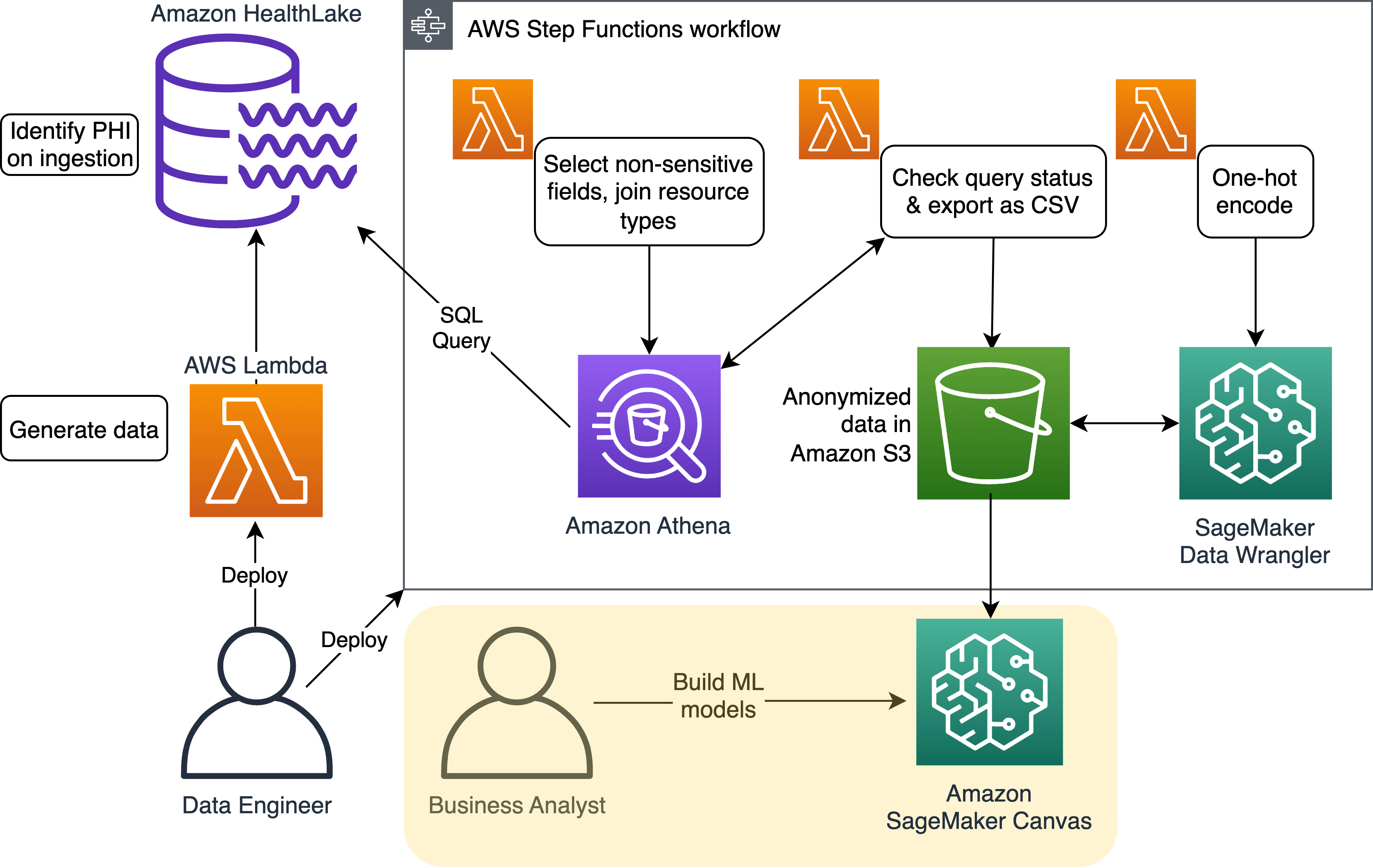
The high-level steps involved in the solution are as follows:

1. Use AWS Step Functions to orchestrate the health data anonymization pipeline.
2. Use Amazon Athena queries for the following:
   1. Extract non-sensitive structured data from Amazon HealthLake.
   2. Use natural language processing (NLP) in Amazon HealthLake to extract non-sensitive data from unstructured blobs.
3. Perform one-hot encoding with Amazon SageMaker Data Wrangler.
4. Use SageMaker Canvas for analytics and predictions.

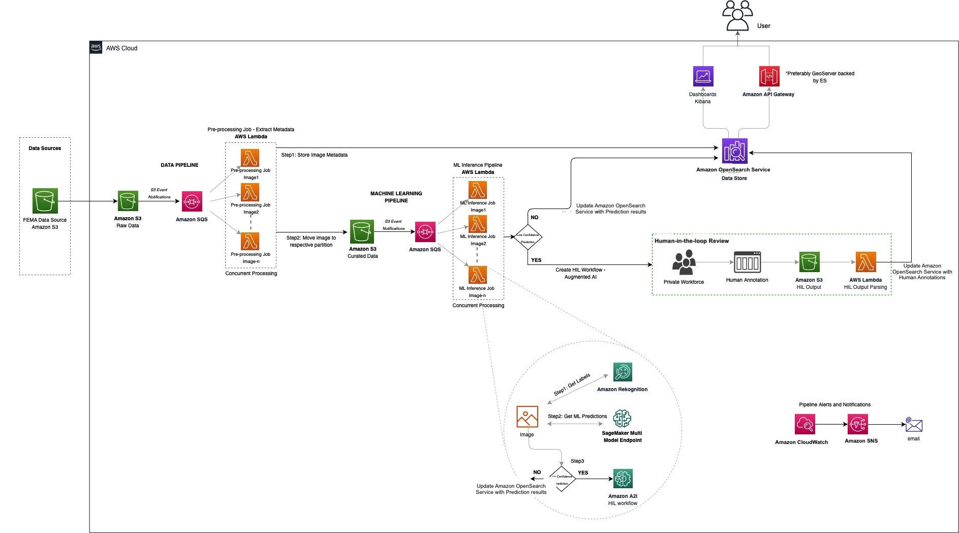
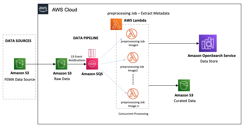
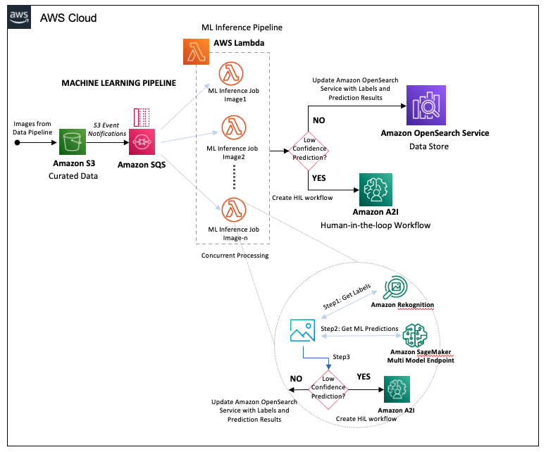
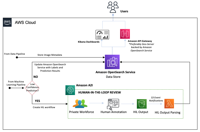
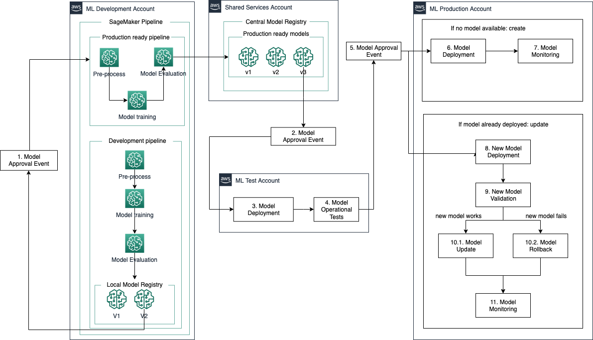
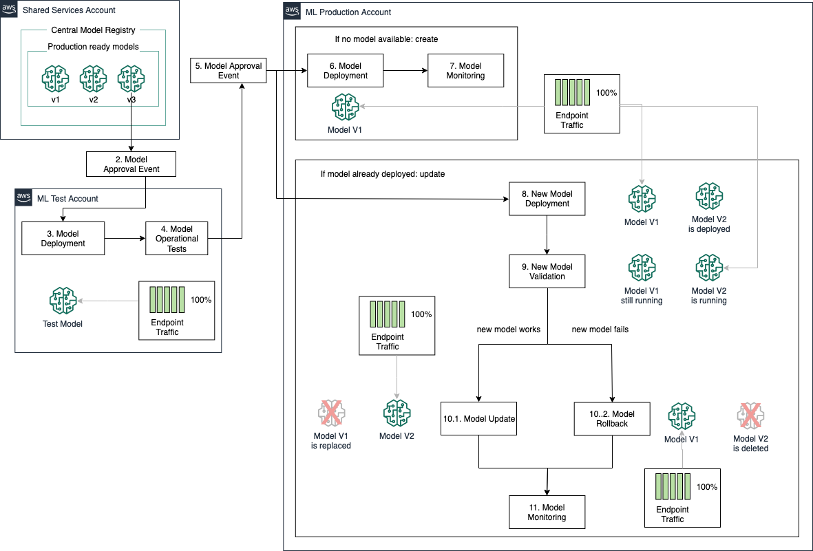
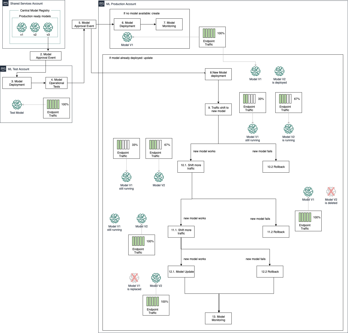
The following diagram illustrates the solution architecture.

Prepare the data

First, we generate a fictional patient population using Synthea and import that data into a newly created Amazon HealthLake data store. The result is a simulation of the starting point from where a healthcare technology company could run the pipeline and solution described in this post.

When Amazon HealthLake ingests data, it automatically extracts meaning from unstructured data, such as doctors notes, into separate structured fields, such as patient names and medical conditions. To accomplish this on the unstructured data in DocumentReference FHIR resources, Amazon HealthLake transparently triggers Amazon Comprehend Medical, where entities, ontologies, and their relationships are extracted and added back to Amazon HealthLake as discreet data within the extension segment of records.

We can use Step Functions to streamline the collection and preparation of the data. The entire workflow is visible in one place, with any errors or exceptions highlighted, allowing for a repeatable, auditable, and extendable process.

Query the data using Athena

By running Athena SQL queries directly on Amazon HealthLake, we are able to select only those fields that are not personally identifying; for example, not selecting name and patient ID, and reducing birthdate to birth year. And by using Amazon HealthLake, our unstructured data (the text field in DocumentReference) automatically comes with a list of detected PHI, which we can use to mask the PHI in the unstructured data. In addition, because generated Amazon HealthLake tables are integrated with AWS Lake Formation, you can control who gets access down to the field level.

The following is an excerpt from an example of unstructured data found in a synthetic DocumentReference record:

# History of Present Illness
Marquis
is a 45 year-old. Patient has a history of hypertension, viral sinusitis (disorder), chronic obstructive bronchitis (disorder), stress (finding), social isolation (finding).
# Social History
Patient is married. Patient quit smoking at age 16.
Patient currently has UnitedHealthcare.
# Allergies
No Known Allergies.
# Medications
albuterol 5 mg/ml inhalation solution; amlodipine 2.5 mg oral tablet; 60 actuat fluticasone propionate 0.25 mg/actuat / salmeterol 0.05 mg/actuat dry powder inhaler
# Assessment and Plan
Patient is presenting with stroke.

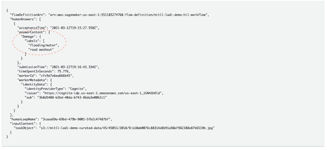
We can see that Amazon HeathLake NLP interprets this as containing the condition “stroke” by querying for the condition record that has the same patient ID and displays “stroke.” And we can take advantage of the fact that entities found in DocumentReference are automatically labeled SYSTEM_GENERATED:

SELECT
  code.coding[1].code,
  code.coding[1].display
FROM
  condition
WHERE
  split(subject.reference, '/')[2] = 'fbfe46b4-70b1-8f61-c343-d241538ebb9b'
AND
  meta.tag[1].display = 'SYSTEM_GENERATED'
AND regexp_like(code.coding[1].display, 'Cerebellar stroke syndrome')

The result is as follows:

G46.4, Cerebellar stroke syndrome

The data collected in Amazon HealthLake can now be effectively used for analytics thanks to the ability to select specific condition codes, such as G46.4, rather than having to interpret entire notes. This data is then stored as a CSV file in Amazon Simple Storage Service (Amazon S3).

Note: When implementing this solution, please follow the instructions on turning on HealthLake’s integrated NLP feature via a support case before ingesting data into your HealthLake data store.

Perform one-hot encoding

To unlock the full potential of the data, we use a technique called one-hot encoding to convert categorical columns, like the condition column, into numerical data.

One of the challenges of working with categorical data is that it is not as amenable to being used in many machine learning algorithms. To overcome this, we use one-hot encoding, which converts each category in a column to a separate binary column, making the data suitable for a wider range of algorithms. This is done using Data Wrangler, which has built-in functions for this:

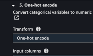
The built-in function for one-hot encoding in SageMaker Data Wrangler

One-hot encoding transforms each unique value in the categorical column into a binary representation, resulting in a new set of columns for each unique value. In the example below, the condition column is transformed into six columns, each representing one unique value. After one-hot encoding, the same rows would turn into a binary representation.

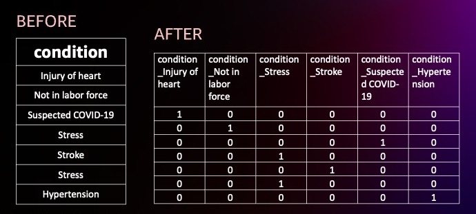
With the data now encoded, we can move on to using SageMaker Canvas for analytics and predictions.

Use SageMaker Canvas for analytics and predictions

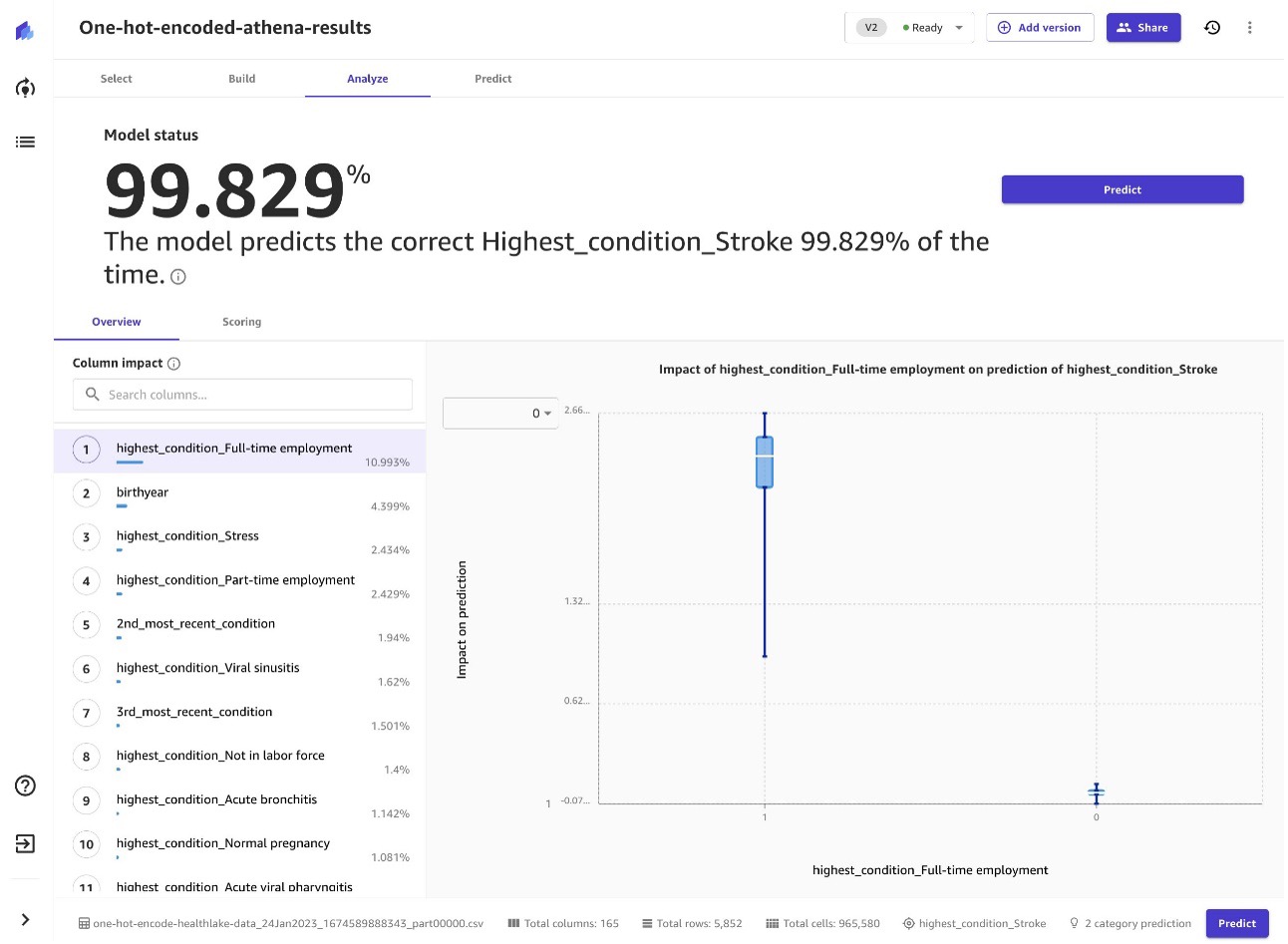
The final CSV file then becomes the input for SageMaker Canvas, which healthcare analysts (business users) can use to generate predictions for multivariate problems like stroke prediction without needing to have expertise in ML. No special permissions are required because the data doesn’t contain any sensitive information.

In the example of stroke prediction, SageMaker Canvas was able to achieve an accuracy rate of 99.829% through the use of advanced ML models, as shown in the following screenshot.

In the next screenshot, you can see that, according to the model’s prediction, this patient has a 53% chance of not having a stroke.

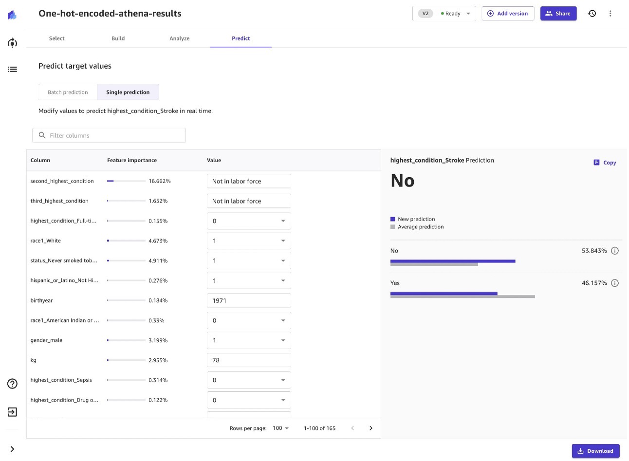
You might posit that you can create this prediction using rule-based logic in a spreadsheet. But do those rules tell you the feature importance—for example, that 4.9% of the prediction is based on whether or not they have ever smoked tobacco? And what if, in addition to the current columns like smoking status and blood pressure, you add 900 more columns (features)? Would you still be able to use a spreadsheet to maintain and manage the combinations of all those dimensions? Real-life scenarios lead to many combinations, and the challenge is to manage this at scale with the right level of effort.

Now that we have this model, we can start making batch or single predictions, asking what-if questions. For example, what if this person keeps all variables the same but, as of the previous two encounters with the medical system, is classified as Full-time employment instead of Not in labor force?

According to our model, and the synthetic data we fed it from Synthea, the person is at a 62% risk of having a stroke.

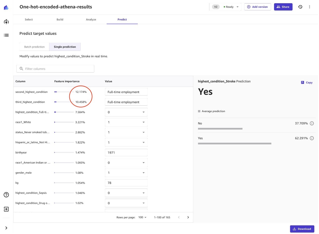
As we can tell from the circled 12% and 10% feature importance of the conditions from the two most recent encounters with the medical system, whether they are full-time employed or not has a big impact on their risk of stroke. Beyond the findings of this model, there is research that demonstrates a similar link:

• “Global, regional, and national burdens of ischemic heart disease and stroke attributable to exposure to long working hours for 194 countries, 2000–2016” (Environment International, 2021)
• “Long working hours and risk of coronary heart disease and stroke: a systematic review and meta-analysis of published and unpublished data for 603 838 individuals” (The Lancet, 2015)
• “Job Strain and the Risk of Stroke: An Individual-Participant Data Meta-Analysis” (Stroke, 2015)

These studies have used large population-based samples and controlled for other risk factors, but it’s important to note that they are observational in nature and do not establish causality. Further research is needed to fully understand the relationship between full-time employment and stroke risk.

Enhancements and alternate methods

To further validate compliance, we can use services like Amazon Macie, which will scan the CSV files in the S3 bucket and alert us if there is any sensitive data. This helps increase the confidence level of the anonymized data.

In this post, we used Amazon S3 as the input data source for SageMaker Canvas. However, we can also import data into SageMaker Canvas directly from Amazon RedShift and Snowflake—popular enterprise data warehouse services used by many customers to organize their data and popular third-party solutions. This is especially important for customers who already have their data in either Snowflake or Amazon Redshift being used for other BI analytics.

By using Step Functions to orchestrate the solution, the solution is more extensible. Instead of a separate trigger to invoke Macie, you can add another step to the end of the pipeline to call Macie to double-check for PHI. If you want to add rules to monitor your data pipeline’s quality over time, you can add a step for AWS Glue Data Quality.

And if you want to add more bespoke integrations, Step Functions lets you scale out to handle as much data or as little data as you need in parallel and only pay for what you use. The parallelization aspect is useful when you are processing hundreds of GB of data, because you don’t want to try to jam all that into one function. Instead, you want to break it up and run it in parallel so you’re not waiting for it to process in a single queue. This is similar to a check-out line at the store—you don’t want to have a single cashier.

Clean up

To avoid incurring future session charges, log out of SageMaker Canvas.

Conclusion

In this post, we showed that predictions for critical health issues like stroke can be done by medical professionals using complex ML models but without the need for coding. This will vastly increase the pool of resources by including people who have specialized domain knowledge but no ML experience. Also, using serverless and managed services allows existing IT people to manage infrastructure challenges like availability, resilience, and scalability with less effort.

You can use this post as a starting point to investigate other complex multi-modal predictions, which are key to guiding the health industry toward better patient care. Coming soon, we will have a GitHub repository to help engineers more quickly launch the kind of ideas we presented in this post.

Experience the power of SageMaker Canvas today, and build your models using a user-friendly graphical interface, with the 2-month Free Tier that SageMaker Canvas offers. You don’t need any coding knowledge to get started, and you can experiment with different options to see how your models perform.

Resources

To learn more about SageMaker Canvas, refer to the following:

• Build, Share, Deploy: how business analysts and data scientists achieve faster time-to-market using no-code ML and Amazon SageMaker Canvas
• Enable intelligent decision-making with Amazon SageMaker Canvas and Amazon QuickSight
• AWS re:Invent 2022 – Better decisions with no-code ML using SageMaker Canvas, feat. Samsung

To learn more about other use cases that you can solve with SageMaker Canvas, check out the following:

• Predict customer churn with no-code machine learning using Amazon SageMaker Canvas
• Reinventing retail with no-code machine learning: Sales forecasting using Amazon SageMaker Canva
• Predict types of machine failures with no-code machine learning using Amazon SageMaker Canvas
• Predict shipment ETA with no-code machine learning using Amazon SageMaker Canvas

To learn more about Amazon HealthLake, refer to the following:

• Get started with Amazon HealthLake
• New Amazon HealthLake capabilities enable next-generation imaging solutions and precision health analytics

About the Authors

Yann Stoneman is a Solutions Architect at AWS based out of Boston, MA and is a member of the AI/ML Technical Field Community (TFC). Yann earned his Bachelors at The Juilliard School. When he’s not modernizing workloads for global enterprises, Yann plays piano, tinkers in React and Python, and regularly YouTubes about his cloud journey.

Ramesh Dwarakanath is a Principal Solutions Architect at AWS based out of Boston, MA. He works with Enterprises in the Northeast area on their Cloud journey. His areas of interest are Containers and DevOps. In his spare time, Ramesh enjoys tennis, racquetball.

Bakha Nurzhanov is an Interoperability Solutions Architect at AWS, and is a member of the Healthcare and Life Sciences technical field community at AWS. Bakha earned his Masters in Computer Science from the University of Washington and in his spare time Bakha enjoys spending time with family, reading, biking, and exploring new places.

Scott Schreckengaust has a degree in biomedical engineering and has been inventing devices alongside scientists on the bench since the beginning of his career. He loves science, technology, and engineering with decades of experiences in startups to large multi-national organizations within the Healthcare and Life Sciences domain. Scott is comfortable scripting robotic liquid handlers, programming instruments, integrating homegrown systems into enterprise systems, and developing complete software deployments from scratch in regulatory environments. Besides helping people out, he thrives on building — enjoying the journey of hashing out customer’s scientific workflows and their issues then converting those into viable solutions.

Read More

Fraud detection is an important problem that has applications in financial services, social media, ecommerce, gaming, and other industries. This post presents an implementation of a fraud detection solution using the Relational Graph Convolutional Network (RGCN) model to predict the probability that a transaction is fraudulent through both the transductive and inductive inference modes. You can deploy our implementation to an Amazon SageMaker endpoint as a real-time fraud detection solution, without requiring external graph storage or orchestration, thereby significantly reducing the deployment cost of the model.

Businesses looking for a fully-managed AWS AI service for fraud detection can also use Amazon Fraud Detector, which you can use to identify suspicious online payments, detect new account fraud, prevent trial and loyalty program abuse, or improve account takeover detection.

Solution overview

The following diagram describes an exemplar financial transaction network that includes different types of information. Each transaction contains information like device identifiers, Wi-Fi IDs, IP addresses, physical locations, telephone numbers, and more. We represent the transaction datasets through a heterogeneous graph that contains different types of nodes and edges. Then, the fraud detection problem is handled as a node classification task on this heterogeneous graph.

Graph neural networks (GNNs) have shown great promise in tackling fraud detection problems, outperforming popular supervised learning methods like gradient-boosted decision trees or fully connected feed-forward networks on benchmarking datasets. In a typical fraud detection setup, during the training phase, a GNN model is trained on a set of labeled transactions. Each training transaction is provided with a binary label denoting if it is fraudulent. This trained model can then be used to detect fraudulent transactions among a set of unlabeled transactions during the inference phase. Two different modes of inference exist: transductive inference vs. inductive inference (which we discuss more later in this post).

GNN-based models, like RGCN, can take advantage of topological information, combining both graph structure and features of nodes and edges to learn a meaningful representation that distinguishes malicious transactions from legitimate transactions. RGCN can effectively learn to represent different types of nodes and edges (relations) via heterogeneous graph embedding. In the preceding diagram, each transaction is being modeled as a target node, and several entities associated with each transaction get modeled as non-target node types, like ProductCD and P_emaildomain. Target nodes have numerical and categorical features assigned, whereas other node types are featureless. The RGCN model learns an embedding for each non-target node type. For the embedding of a target node, a convolutional operation is used to compute its embedding using its features and neighborhood embeddings. In the rest of the post, we use the terms GNN and RGCN interchangeably.

It’s worth noting that alternative strategies, such as treating the non-target entities as features and one-hot-encoding them, would often be infeasible because of the large cardinalities of these entities. Conversely, encoding them as graph entities enables the GNN model to take advantage of the implicit topology in the entity relationships. For example, transactions that share a phone number with known fraudulent transactions are more likely to be fraudulent too.

The graph representation employed by GNNs creates some complexity in their implementation. This is especially true for applications such as fraud detection, in which the graph representation may get augmented during inference with newly added nodes that correspond to entities not known during model training. This inference scenario is usually referred to as inductive mode. In contrast, transductive mode is a scenario that assumes the graph representation constructed during model training won’t change during inference. GNN models are often evaluated in transductive mode by constructing graph representations from a combined set of training and test examples, while masking test labels during back-propagation. This ensures the graph representation is static, and there the GNN model doesn’t require implementation of operations to extend the graph with new nodes during inference. Unfortunately, static graph representation can’t be assumed when detecting fraudulent transactions in a real-world setting. Therefore, support for inductive inference is required when deploying GNN models for fraud detection to production environments.

In addition, detecting fraudulent transactions in real time is crucial, especially in business cases where there is only one chance of stopping illegal activities. For example, fraudulent users can behave maliciously just once with an account and never use the same account again. Real-time inference on GNN models introduces additional complexity to the implementation. It is often necessary to implement subgraph extraction operations to support real-time inference. The subgraph extraction operation is needed to reduce inference latency when graph representation is large and performing inference on the entire graph becomes prohibitively expensive. An algorithm for real-time inductive inference with an RGCN model runs as follows:

1. Given a batch of transactions and a trained RGCN model, extend graph representation with entities from the batch.
2. Assign embedding vectors of new non-target nodes with the mean embedding vector of their respective node type.
3. Extract a subgraph induced by k-hop out-neighborhood of the target nodes from the batch.
4. Perform inference on the subgraph and return prediction scores for the batch’s target nodes.
5. Clean up the graph representation by removing newly added nodes (this step ensures the memory requirement for model inference stays constant).

The key contribution of this post is to present an RGCN model implementing the real-time inductive inference algorithm. You can deploy our RGCN implementation to a SageMaker endpoint as a real-time fraud detection solution. Our solution doesn’t require external graph storage or orchestration, and significantly reduces the deployment cost of the RGCN model for fraud detection tasks. The model also implements transductive inference mode, enabling us to carry out experiments to compare model performance in inductive and transductive modes. The model code and notebooks with experiments can be accessed from the AWS Examples GitHub repo.

This post builds on the post Build a GNN-based real-time fraud detection solution using Amazon SageMaker, Amazon Neptune, and the Deep Graph Library. The previous post built a RGCN-based real-time fraud detection solution using SageMaker, Amazon Neptune, and the Deep Graph Library (DGL). The prior solution used a Neptune database as external graph storage, required AWS Lambda for orchestration for real-time inference, and only included experiments in transductive mode.

The RGCN model introduced in this post implements all operations of the real-time inductive inference algorithm using only the DGL as a dependency, and doesn’t require external graph storage or orchestration for deployment.

We first evaluate the performance of the RGCN model in transductive and inductive modes on a benchmark dataset. As expected, model performance in inductive mode is slightly lower than in transductive mode. We also study the effect of hyperparameter k on model performance. The hyperparameter k controls the number of hops performed to extract a subgraph in Step 3 of the real-time inference algorithm. Higher values of k will produce larger subgraphs and can lead to better inference performance at the expense of higher latency. As such, we also conduct timing experiments to evaluate the feasibility of the RGCN model for a real-time application.

Dataset

We use the IEEE-CIS fraud dataset, the same dataset that was used in the previous post. The dataset contains over 590,000 transaction records that have a binary fraud label (the isFraud column). The data is split into two tables: transaction and identity. However, not all transaction records have corresponding identity information. We join the two tables on the TransactionID column, which leaves us with a total of 144,233 transaction records. We sort the table by transaction timestamp (the TransactionDT column) and create an 80/20 percentage split by time, producing 115,386 and 28,847 transactions for training and testing, respectively.

For more details on the dataset and how to format it to suit the input requirement of the DGL, refer to Detecting fraud in heterogeneous networks using Amazon SageMaker and Deep Graph Library.

Graph construction

We use the TransactionID column to generate target nodes. We use the following columns to generate 11 types of non-target nodes:

• card1 through card6
• ProductCD
• addr1 and addr2
• P_emaildomain and R_emaildomain

We use 38 columns as categorical features of target nodes:

• M1 through M9
• DeviceType and DeviceInfo
• id_12 through id_38

We use 382 columns as numerical features of target nodes:

• TransactionAmt
• dist1 and dist2
• id_01 through id_11
• C1 through C14
• D1 through D15
• V1 through V339

Our graph constructed from the training transactions contains 217,935 nodes and 2,653,878 edges.

Hyperparameters

Other parameters are set to match the parameters reported in the previous post. The following snippet illustrates training the RGCN model in transductive and inductive modes:

import pandas as pd
from fgnn.fraud_detector import FraudRGCN

# overload default hyperparameters defined in FraudRGCN constructor
params = {
    "embedding_size": 64,
    "n_layers": 2,
    "n_epochs": 150,
    "n_hidden": 16,
    "dropout": 0.2,
    "weight_decay": 5e-05,
    "lr": 0.01
}

# load train and test splits
df_train = pd.read_parquet('./data/train.parquet')
df_test = pd.read_parquet('./data/test.parquet')

# train RGCN model in inductive mode
fd_ind = FraudRGCN()
fd_ind.train_fg(df_train, params=params)

# train RGCN model in transductive mode
fd_trs = FraudRGCN()
# create boolean array to identify test examples
test_mask = [False]*len(df_train) + [True]*len(df_test)
# concatenate train and test examaples
df_combined = pd.concat([df_train, df_test], ignore_index=True)	
# test_mask must be passed in transductive mode, 
# so test labels are masked-out during back-propagation
fd.train_fg(df_combined, params=params, test_mask=test_mask)

# predict on both models extracting subgraph with 2 k-hops
fraud_proba_ind = fd_ind.predict(df_test, k=2)
fraud_proba_trs = fd_trs.predict(df_test, k=2)

Inductive vs. transductive mode

We perform five trials for inductive and five trials for transductive mode. For each trial, we train an RGCN model and save it to disk, obtaining 10 models. We evaluate each model on test examples while increasing the number of hops (parameter k) used to extract a subgraph for inference, setting k to 1, 2, and 3. We predict on all test examples at once, and compute the ROC AUC score for each trial. The following plot shows the mean and 95% confidence intervals of AUC scores.

We can see that performance in transductive mode is slightly higher than in inductive mode. For k=2, mean AUC scores for inductive and transductive modes are 0.876 and 0.883, respectively. This is expected because the RGCN model is able to learn embeddings of all entity nodes in transductive mode, including those in the test set. In contrast, inductive mode only allows the model to learn embeddings of entity nodes that are present in the training examples, and therefore some nodes have to be mean-filled during inference. At the same time, the drop in performance between transductive and inductive modes is not significant, and even in inductive mode, the RGCN model achieves good performance with an AUC of 0.876. We also observe that model performance doesn’t improve for values of k>2. This implies that setting k=2 would extract a sufficiently large subgraph during inference, resulting in optimal performance. This observation is also confirmed by our next experiment.

It’s also worth noting that, for transductive mode, our model’s AUC of 0.883 is higher than the corresponding AUC of 0.870 reported in the previous post. We use more columns as numerical and categorical features of target nodes, which can explain the higher AUC score. We also note that the experiments in the previous post only performed a single trial.

Inference on a small batch

For this experiment, we evaluate the RGCN model in a small batch inference setting. We use five models that were trained in inductive mode in the previous experiment. We compare performance of these models when predicting in two settings: full and small batch inference. For full batch inference, we predict on the entire test set, as was done in the previous experiment. For small batch inference, we predict in small batches by partitioning the test set into 28 batches of equal size with approximately 1,000 transactions in each batch. We compute AUC scores for both settings using different values of k. The following plot shows the mean and 95% confidence intervals for full and small batch inference settings.

We observe that performance for small batch inference when k=1 is lower than for full batch. However, small batch inference performance matches full batch when k>1. This can be attributed to much smaller subgraphs being extracted for small batches. We confirm this by comparing subgraph sizes with the size of the entire graph constructed from the training transactions. We compare graph sizes in terms of number of nodes. For k=1, the average subgraph size for small batch inference is less than 2% of the training graph. And for full batch inference when k=1, the subgraph size is 22%. When k=2, subgraph sizes for small and full batch inference are 54% and 64%, respectively. Finally, subgraph sizes for both inference settings reach 100% for k=3. In other words, when k>1, the subgraph for a small batch becomes sufficiently large, enabling small batch inference to reach the same performance as full batch inference.

We also record prediction latency for every batch. We perform our experiments on an ml.r5.12xlarge instance, but you can use a smaller instance with 64 G memory to run the same experiments. The following plot shows the mean and 95% confidence intervals of small batch prediction latencies for different values of k.

The latency includes all five steps of the real-time inductive inference algorithm. We see that when k=2, predicting on 1,030 transactions takes 5.4 seconds on average, resulting in a throughput of 190 transactions per second. This confirms that the RGCN model implementation is suitable for real-time fraud detection. We also note that the previous post did not provide hard latency values for their implementation.

Conclusion

The RGCN model released with this post implements the algorithm for real-time inductive inference, and doesn’t require external graph storage or orchestration. The parameter k in Step 3 of the algorithm specifies the number of hops performed to extract the subgraph for inference, and results in a trade-off between model accuracy and prediction latency. We used the IEEE-CIS fraud dataset in our experiments, and empirically validated that the optimal value of parameter k for this dataset is 2, achieving an AUC score of 0.876 and prediction latency of less than 6 seconds per 1,000 transactions.

This post provided a step-by-step process for training and evaluating an RGCN model for real-time fraud detection. The included model class implements methods for the entire model lifecycle, including serialization and deserialization methods. This enables the model to be used for real-time fraud detection. You can train the model as a PyTorch SageMaker estimator and then deploy it to a SageMaker endpoint by using the following notebook as a template. The endpoint is able to predict fraud on small batches of raw transactions in real time. You can also use Amazon SageMaker Inference Recommender to select the best instance type and configuration for the inference endpoint based on your workloads.

For more information about this topic and implementation, we encourage you to explore and test our scripts on your own. You can access the notebooks and related model class code from the AWS Examples GitHub repo.

About the Authors

Dmitriy Bespalov is a Senior Applied Scientist at the Amazon Machine Learning Solutions Lab, where he helps AWS customers across different industries accelerate their AI and cloud adoption.

Ryan Brand is an Applied Scientist at the Amazon Machine Learning Solutions Lab. He has specific experience in applying machine learning to problems in healthcare and life sciences. In his free time, he enjoys reading history and science fiction.

Yanjun Qi is a Senior Applied Science Manager at the Amazon Machine Learning Solution Lab. She innovates and applies machine learning to help AWS customers speed up their AI and cloud adoption.

Read More

Model tuning is the experimental process of finding the optimal parameters and configurations for a machine learning (ML) model that result in the best possible desired outcome with a validation dataset. Single objective optimization with a performance metric is the most common approach for tuning ML models. However, in addition to predictive performance, there may be multiple objectives which need to be considered for certain applications. For example,

1. Fairness – The aim here is to encourage models to mitigate bias in model outcomes between certain sub-groups in the data, especially when humans are subject to algorithmic decisions. For example, a credit lending application should not only be accurate but also unbiased to different population sub-groups.
2. Inference time – The aim here is to reduce the inference time during model invocation. For example, a speech recognition system must not only understand different dialects of the same language accurately, but also operate within a specified time limit that is acceptable by the business process.
3. Energy efficiency – The aim here is to train smaller energy-efficient models. For example, neural network models are compressed for usage on mobile devices and thus naturally reduce their energy consumption by reducing the number of FLOPS required for a pass through the network.

Multi-objective optimization methods represent different trade-offs between the desired metrics. This can involve finding a global minimum of an objective function subject to a set of constraints on different metrics being simultaneously satisfied.

Amazon SageMaker Automatic Model Tuning (AMT) finds the best version of a model by running many SageMaker training jobs on your dataset using the algorithm and ranges of hyperparameters. It then chooses the hyperparameter values that result in a model that performs the best, as measured by a metric (e.g., accuracy, auc, recall) that you define. With Amazon SageMaker automatic model tuning, you can find the best version of your model by running training jobs on your dataset with several search strategies, such as Bayesian, Random search, Grid search, and Hyperband.

Amazon SageMaker Clarify can detect potential bias during data preparation, after model training, and in your deployed model. Currently, it offers 21 different metrics to choose from. These metrics are also openly available with the smclarify python package and github repository here. You can learn more about measuring bias with metrics from Amazon SageMaker Clarify at Learn how Amazon SageMaker Clarify helps detect bias.

In this blog we show you how to automatically tune a ML model with Amazon SageMaker AMT for both accuracy and fairness objectives by creating a single combined metric. We demonstrate a financial services use case of credit risk prediction with an accuracy metric of Area Under the Curve (AUC) to measure performance and a bias metric of Difference in Positive Proportions in Predicted Labels (DPPL) from SageMaker Clarify to measure the imbalance in model predictions for different demographic groups. The code for this example is available on GitHub.

Fairness in Credit Risk prediction

The credit lending industry relies heavily on credit scores for processing loan applications. Generally, credit scores reflect an applicant’s history of borrowing and paying back money, and lenders refer to them when determining an individual’s creditworthiness. Payment firms and banks are interested to build systems that can help identify the risk associated with a particular application and provide competitive credit products. Machine learning (ML) models can be used to build such a system that processes historical applicant data and predicts the credit risk profile. Data can include financial and employment history of the applicant, their demographics, and the new credit/loan context. There is always some statistical uncertainty with any model that predicts whether a particular applicant will default in the future. The systems need to provide a tradeoff between rejecting applications that might default over time and accepting applications that are eventually creditworthy.

Business owners of such a system need to ensure the validity and quality of the models as per existing and upcoming regulatory compliance requirements. They are obligated to treat customers fairly and provide transparency in their decision making. They might want to ensure that positive model predictions are not imbalanced across different groups (for example, gender, race, ethnicity, immigration status and others). Once the required data is collected, the ML model training typically optimizes for prediction performance as a primary objective with a metric like classification accuracy or AUC score. Alternatively, a model with a given performance objective can be constrained with a fairness metric to ensure certain requirements are maintained. One such technique to constrain the model is fairness-aware hyperparameter tuning. By applying these strategies, the best candidate model can have lower bias than the unconstrained model while maintaining a high predictive performance.

In the scenario depicted in this schematic,

1. The ML model is built with historical customer credit profile data. The model training and hyperparameter tuning process maximizes for multiple objectives including classification accuracy and fairness. The model is deployed to an existing business process in a production system.
2. A new customer credit profile is evaluated for credit risk. If low risk, it can go through an automated process. High risk applications could include human review before a final acceptance or rejection decision.

The decisions and metrics gathered during design and development, deployment and operations can be documented with SageMaker Model Cards and shared with the stakeholders.

This use case demonstrates how to reduce model bias against a specific group by fine tuning hyperparameters for a combined objective metric of both accuracy and fairness with SageMaker Automatic Model Tuning. We use the South German Credit dataset (South German Credit Data Set) .

The applicant data can be split into following categories:

1. Demographic
2. Financial Data
3. Employment History
4. Loan purpose

In this example, we specifically look at the ‘Foreign worker’ demographic and tune a model that predicts credit application decisions with high accuracy and low bias against that particular subgroup.

There are various bias metrics that can be used to evaluate fairness of the system with respect to specific sub-groups in the data. Here, we use the absolute value of Difference in Positive Proportions in Predicted Labels (DPPL) from SageMaker Clarify. In simple terms, DPPL measures the difference in positive class (good credit) assignments between non-foreign workers and foreign workers.

For example, if 4.5% of all foreign workers are assigned the positive label by the model, and 13.7% of all non-foreign workers are assigned the positive label, then DPPL = 0.137 – 0.045 = 0.092.

Solution Architecture

The figure below displays a high level overview of the architecture of an Automatic Model Tuning job with XGBoost on Amazon SageMaker.

In the solution, SageMaker Processing preprocesses the training dataset from Amazon S3. Amazon SageMaker Automatic Tuning instantiates multiple SageMaker training jobs with their associated EC2 instances and EBS volumes. The container for the algorithm (XGBoost) is loaded from Amazon ECR in each job. SageMaker AMT finds the best version of a model by running many training jobs on the preprocessed dataset using the specified algorithm script and range of hyperparameters. The output metrics are logged in Amazon CloudWatch for monitoring.

The hyperparameters we are tuning in this use case are as follows:

1. eta – Step size shrinkage used in updates to prevent overfitting.
2. min_child_weight – Minimum sum of instance weight (hessian) needed in a child.
3. gamma – Minimum loss reduction required to make a further partition on a leaf node of the tree.
4. max_depth – Maximum depth of a tree.

The definition of these hyperparameters and others available with SageMaker AMT can be found here.

First, we demonstrate a baseline scenario of a single performance objective metric for tuning hyperparameters with Automatic Model Tuning. Then, we demonstrate the optimized scenario of a multi-objective metric specified as a combination of performance metric and fairness metric.

Single Metric Hyperparameter Tuning (Baseline)

There is a choice of multiple metrics for a tuning job to evaluate the individual training jobs. As per the code snippet below, we specify the single objective metric as  objective_metric_name. The hyperparameter tuning job returns the training job that gave the best value for the chosen objective metric.

In this baseline scenario, we are tuning for Area Under Curve (AUC) as seen below. It is important to note that we are only optimizing AUC, and not optimizing for other metrics such as fairness.

from sagemaker.tuner import IntegerParameter, CategoricalParameter, ContinuousParameter, HyperparameterTuner

hyperparameter_ranges = {'eta': ContinuousParameter(0, 1),
'min_child_weight': IntegerParameter(1, 10),
'gamma': IntegerParameter(1, 5),
'max_depth': IntegerParameter(1, 10)}

objective_metric_name = 'validation:auc'

tuner = HyperparameterTuner(estimator,
objective_metric_name,
hyperparameter_ranges,
max_jobs=100,
max_parallel_jobs=10,
)

tuning_job_name = "xgb-tuner-{}".format(strftime("%d-%H-%M-%S", gmtime()))
inputs = {'train': train_data_path, 'validation': val_data_path}
tuner.fit(inputs, job_name=tuning_job_name)
tuner.wait()
tuner_metrics = sagemaker.HyperparameterTuningJobAnalytics(tuning_job_name)

In this context max jobs allows us to specify how many times a single training job will be tuned, and finding the best training job from there.

Multi Objective Hyperparameter Tuning (Fairness Optimized)

We want to optimize multiple objective metrics with hyperparameter tuning as described in this paper. However, SageMaker AMT still accepts only a single metric as input.

To address this challenge, we express multiple metrics as a single metric function and optimize this metric:

• maxM(y1​,y2​,θ)
• y1​,y2​ are different metrics. For example AUC score and DPPL.
• M(⋅,⋅,θ)is a scalarization function and is parameterized by a fixed parameter

Higher weight favors that particular objective in model tuning. Weights may wary from case to case and you might need to try different weights for your use case. In this example, weights for AUC and DPPL have been set heuristically. Let’s walk through how this would look like in code. You can see the training job returning a single metric based on a combination function of AUC Score for performance and DPPL for fairness. The hyperparameter optimization ranges for multiple objectives are the same as the single objective. We are passing the validation metric as “auc” but behind the scenes we are returning the results of the combined metric function as described last in the list of functions below:

Here is the function Multi Objective optimization:

objective_metric_name = 'validation:auc'
tuner = HyperparameterTuner(estimator,
                            objective_metric_name,
                            hyperparameter_ranges,
                            max_jobs=100,
                            max_parallel_jobs=10
                           )

Here is the function for computing AUC score:

def eval_auc_score(predt, dtrain):
   fY = [1 if p > 0.5 else 0 for p in predt]
   y = dtrain.get_label()
   auc_score = roc_auc_score(y, fY)
   return auc_score

Here is the function for computing DPPL score:

def eval_dppl(predt, dtrain):
    dtrain_np = dmatrix_to_numpy(dtrain)
    # groups: an np array containing 1 or 2
    groups = dtrain_np[:, -1]
    # sensitive_facet_index: boolean column indicating sensitive group
    sensitive_facet_index = pd.Series(groups - 1, dtype=bool)
    # positive_predicted_label_index: boolean column indicating positive predicted labels
    positive_label_index = pd.Series(predt > 0.5)
    return abs(DPPL(predt, sensitive_facet_index, positive_label_index))

Here is the function for the Combined Metric:

def eval_combined_metric(predt, dtrain):
    auc_score = eval_auc_score(predt, dtrain)
    DPPL = eval_dppl(predt, dtrain)
    # Assign weight of 3 to AUC and 1 to DPPL
    # Maximize (1-DPPL) for the purpose of minimizing DPPL 
    combined_metric = ((3*auc_score)+(1-DPPL))/4       
    print("DPPL, AUC Score, Combined Metric: ", DPPL, auc_score, combined_metric)
    return "auc", combined_metric

Experiments & Results

Synthetic data generation for bias dataset

The original South German Credit dataset contained 1000 records, and we generated 100 more records synthetically to create a dataset where the bias in model predictions disfavors Foreign Workers. This is done to simulate bias that could manifest itself in the real world. New records of foreign workers labeled as “bad credit” applicants were extrapolated from existing foreign workers with the same label.

There are many libraries/techniques to create synthetic data and we use Synthetic Data Vault (DPPLV).

From the following code snippet we can see how synthetic data is generated with DPPLV with the South German Credit Data Set:

# Parameters for generated data
# How many rows of synthetic data
num_rows = 100

# Select all foreign workers who were accepted (foreign_worker value 1 credit_risk 1)
ForeignWorkerData = training_data.loc[(training_data['foreign_worker'] == 1) & (training_data['credit_risk'] == 1)]

# Fit Foreign Worker data to SDV model
model = GaussianCopula()
model.fit(ForeignWorkerData)

# Generate Synthetic foreign worker data based on rows stated
SynthForeignWorkers = model.sample(Rows)

We generated 100 new synthetic records of Foreign Workers based on Foreign Workers who were accepted in the original dataset. We will now take those records and convert the “credit_risk” label to 0 (bad credit). This will mark these Foreign Workers unfairly as bad credit, hence inserting bias into our dataset

SynthForeignWorkers.loc[SynthForeignWorkers['credit_risk'] == 1, 'credit_risk'] = 0

We explore the bias in the dataset through the graphs below.

The pie graph on top shows the percentage of Non-Foreign Workers labelled as good credit or bad credit, and the bottom pie graph shows the same for Foreign Workers. The percentage of Foreign workers labeled as  “bad credit” is 75.90% and far outweigh the 30.70% of Non-Foreign workers labeled the same. The stack bar displays the almost similar percentage breakdown of total workers across the category of Foreign & Non-Foreign workers.

We want to avoid the ML model from learning a strong bias against Foreign Workers either through explicit features or implicit proxy features in the data. With an additional fairness objective, we guide the ML model to mitigate the bias of lower creditworthiness towards Foreign Workers.

Model performance after tuning for both performance and fairness

This chart depicts the density plot of up to 100 tuning jobs run by SageMaker AMT and their corresponding combined objective metric values. Although we have set max jobs to 100, it is changeable under the discretion of the user. The combined metric was a combination of AUC and DPPL with a function of: (3*AUC + (1-DPPL)) / 4. The reason that we use (1-DPPL) instead of (DPPL) is because we would like to maximize the combined objective for the lowest DPPL possible (lower DPPL means lower bias against foreign workers). The plot shows how AMT helps identify the best hyperparameters for the XGBoost model that returns the highest combined evaluation metric value of 0.68.

Model performance with combined metric

Below we take a look at the pareto front chart for the individual metrics of AUC and DPPL. A Pareto Front chart is used here to visually represent the trade-offs between multiple objectives, in this case the two metric values (AUC & DPPL). Points on the curve front are considered as equally good and one metric cannot be improved without degrading the other. The Pareto chart allows us to see how different jobs performed against the baseline (red circle) in terms of both metrics. It also shows us the most optimal job (green triangle). The position of the red circle and green triangle are important because it allows us to understand if our combined metric is actually performing as expected and truly optimizing for both metrics. The code to generate the pareto front chart is included in the notebook in GitHub.

In this scenario, a lower DPPL value is more desirable (less bias), while higher AUC is better (increased performance).

Here, the baseline (red circle) represents the scenario where the objective metric is AUC alone. In other words, the baseline does not consider DPPL at all and optimizes only for AUC (no fine tuning for fairness). We see the baseline has a good AUC score of 0.74, but does not perform well on fairness with a DPPL score of 0.75.

The Optimized model (green triangle) represents the best candidate model when fine-tuned for a combined metric with weight ratio of 3:1 for AUC:DPPL. We see the optimized model has a good AUC score of 0.72, and also a low DPPL score of 0.43 (low bias). This tuning job found a model configuration where DPPL can be significantly lower than the baseline, without a significant drop in AUC.  Models with even lower DPPL scores can be identified by moving the green triangle further left along the Pareto Front. We thus achieved the combined objective of a well performing model with fairness for Foreign Worker sub-groups.

In the chart below, we can see the results of the predictions from the baseline model and the optimized model. The optimized model with a combined objective of performance and fairness predicts a positive outcome for 30.6% Foreign Workers as opposed to the 13.9% from the baseline model. The optimized model thus reduces the model bias against this sub-group.

Conclusion

The blog shows you to implement multi-objective optimization with SageMaker Automatic Model Tuning for real-world applications. In many instances, collected data in the real world may be biased against certain subgroups. Multi-objective optimization using automatic model tuning enables customers to build ML models easily that optimize fairness in addition to accuracy. We demonstrate an example of credit risk prediction and specifically look at fairness for foreign workers. We show that it is possible to maximize for another metric like fairness while continuing to train models with high performance. If what you have read has piqued your interest you may try out the code example hosted in Github here.

About the authors

Munish Dabra is a Senior Solutions Architect at Amazon Web Services (AWS). His current areas of focus are AI/ML, Data Analytics and Observability. He has a strong background in designing and building scalable distributed systems. He enjoys helping customers innovate and transform their business in AWS. LinkedIn: /mdabra

Hasan Poonawala is a Senior AI/ML Specialist Solutions Architect at AWS, Hasan helps customers design and deploy machine learning applications in production on AWS. He has over 12 years of work experience as a data scientist, machine learning practitioner, and software developer. In his spare time, Hasan loves to explore nature and spend time with friends and family.

Mohammad (Moh) Tahsin is an associate AI/ML Specialist Solutions Architect for AWS. Moh has experience teaching students about responsible AI concepts, and is passionate about conveying these concepts through cloud based architectures. In his spare time he loves to lift weights, play games, and explore nature.

Xingchen Ma is an Applied Scientist at AWS. He works in service team for SageMaker Automatic Model Tuning.

Rahul Sureka is an Enterprise Solution Architect at AWS based out of India. Rahul has more than 22 years of experience in architecting and leading large business transformation programs across multiple industry segments. His areas of interests are data and analytics, streaming, and AI/ML applications.

Read More

In recent years, advances in computer vision have enabled researchers, first responders, and governments to tackle the challenging problem of processing global satellite imagery to understand our planet and our impact on it. AWS recently released Amazon SageMaker geospatial capabilities to provide you with satellite imagery and geospatial state-of-the-art machine learning (ML) models, reducing barriers for these types of use cases. For more information, refer to Preview: Use Amazon SageMaker to Build, Train, and Deploy ML Models Using Geospatial Data.

Many agencies, including first responders, are using these offerings to gain large-scale situational awareness and prioritize relief efforts in geographical areas that have been struck by natural disasters. Often these agencies are dealing with disaster imagery from low altitude and satellite sources, and this data is often unlabeled and difficult to use. State-of-the-art computer vision models often underperform when looking at satellite images of a city that a hurricane or wildfire has hit. Given the lack of these datasets, even state-of-the-art ML models are often unable to deliver the accuracy and precision required to predict standard FEMA disaster classifications.

Geospatial datasets contain useful metadata such as latitude and longitude coordinates, and timestamps, which can provide context for these images. This is especially helpful in improving the accuracy of geospatial ML for disaster scenes, because these images are inherently messy and chaotic. Buildings are less rectangular, vegetation has sustained damage, and linear roads have been interrupted by flooding or mudslides. Because labeling these massive datasets is expensive, manual, and time-consuming, the development of ML models that can automate image labeling and annotation is critical.

To train this model, we need a labeled ground truth subset of the Low Altitude Disaster Imagery (LADI) dataset. This dataset consists of human and machine annotated airborne images collected by the Civil Air Patrol in support of various disaster responses from 2015-2019. These LADI datasets focus on the Atlantic hurricane seasons and coastal states along the Atlantic Ocean and Gulf of Mexico. Two key distinctions are the low altitude, oblique perspective of the imagery and disaster-related features, which are rarely featured in computer vision benchmarks and datasets. The teams used existing FEMA categories for damage such as flooding, debris, fire and smoke, or landslides, which standardized the label categories. The solution is then able to make predictions on the rest of the training data, and route lower-confidence results for human review.

In this post, we describe our design and implementation of the solution, best practices, and the key components of the system architecture.

Solution overview

In brief, the solution involved building three pipelines:

• Data pipeline – Extracts the metadata of the images
• Machine learning pipeline – Classifies and labels images
• Human-in-the-loop review pipeline – Uses a human team to review results

The following diagram illustrates the solution architecture.

Given the nature of a labeling system like this, we designed a horizontally scalable architecture that would handle ingestion spikes without over-provisioning by using a serverless architecture. We use a one-to-many pattern from Amazon Simple Queue Service (Amazon SQS) to AWS Lambda in multiple spots to support these ingestion spikes, offering resiliency.

Using an SQS queue for processing Amazon Simple Storage Service (Amazon S3) events helps us control the concurrency of downstream processing (Lambda functions, in this case) and handle the incoming spikes of data. Queuing incoming messages also acts as a buffer storage in case of any failures downstream.

Given the highly parallel needs, we chose Lambda to process our images. Lambda is a serverless compute service that lets us run code without provisioning or managing servers, creating workload-aware cluster scaling logic, maintaining event integrations, and managing runtimes.

We use Amazon OpenSearch Service as our central data store to take advantage of its highly scalable, fast searches and integrated visualization tool, OpenSearch Dashboards. It enables us to iteratively add context to the image, without having to recompile or rescale, and handle schema evolution.

Amazon Rekognition makes it easy to add image and video analysis into our applications, using proven, highly scalable, deep learning technology. With Amazon Rekognition, we get a good baseline of detected objects.

In the following sections, we dive into each pipeline in more detail.

Data pipeline

The following diagram shows the workflow of the data pipeline.

The LADI data pipeline starts with the ingestion of raw data images from the FEMA Common Alerting Protocol (CAP) into an S3 bucket. As we ingest the images into the raw data bucket, they are processed in near-real time in two steps:

1. The S3 bucket triggers event notifications for all object creations, creating messages in the SQS queue for each image ingested.
2. The SQS queue concurrently invokes the preprocessing Lambda functions on the image.

The Lambda functions perform the following preprocessing steps:

3. Compute the UUID for each image, providing a unique identifier for each image. This ID will identify the image for its entire lifecycle.
4. Extract metadata such as GPS coordinates, image size, GIS information, and S3 location from the image and persist it into OpenSearch.
5. Based on a lookup against FIPS codes, the function moves the image into the curated data S3 bucket. We partition the data by the image’s FIPS-State-code/FIPS-County-code/Year/Month.

Machine learning pipeline

The ML pipeline starts from the images landing in the curated data S3 bucket in the data pipeline step, which triggers the following steps:

1. Amazon S3 generates a message into another SQS queue for each object created in the curated data S3 bucket.
2. The SQS queue concurrently triggers Lambda functions to run the ML inference job on the image.

The Lambda functions perform the following actions:

3. Send each image to Amazon Rekognition for object detection, storing the returned labels and respective confidence scores.
4. Compose the Amazon Rekognition output into input parameters for our Amazon SageMaker multi-model endpoint. This endpoint hosts our ensemble of classifiers, which are trained for specific sets of damage labels.
5. Pass the results of the SageMaker endpoint to Amazon Augmented AI (Amazon A2I).

The following diagram illustrates the pipeline workflow.

Human-in-the-loop review pipeline

The following diagram illustrates the human-in-the-loop (HIL) pipeline.

With Amazon A2I, we can configure thresholds that will trigger a human review by a private team when a model yields a low confidence prediction. We can also use Amazon A2I to provide an ongoing audit of our model’s predictions. The workflow steps are as follows:

1. Amazon A2I routes high confidence predictions into OpenSearch Service, updating the image’s label data.
2. Amazon A2I routes low confidence predictions to the private team to annotate images manually.
3. The human reviewer completes the annotation, generating a human annotation output file that is stored in the HIL Output S3 bucket.
4. The HIL Output S3 bucket triggers a Lambda function that parses the human annotations output and updates the image’s data in OpenSearch Service.

By routing the human annotation results back to the data store, we can retrain the ensemble models and iteratively improve the model’s accuracy.

With our high-quality results now stored in OpenSearch Service, we’re able to perform geospatial and temporal search via a REST API, using Amazon API Gateway and Geoserver. OpenSearch Dashboard also enables users to search and run analytics with this dataset.

Results

The following code shows an example of our results.

With this new pipeline, we create a human backstop for models that are not yet fully performant. This new ML pipeline has been put into production for use with a Civil Air Patrol Image Filter microservice that allows for filtering of Civil Air Patrol images in Puerto Rico. This enables first responders to view the extent of damage and view images associated with that damage following hurricanes. The AWS Data Lab, AWS Open Data Program, Amazon Disaster Response team, and AWS human-in-the-loop team worked with customers to develop an open-source pipeline that can be used to analyze Civil Air Patrol data stored in the Open Data Program registry on demand following any natural disaster. For more information about the pipeline architecture and an overview of the collaboration and impact, check out the video Focusing on disaster response with Amazon Augmented AI, the AWS Open Data Program and AWS Snowball.

Conclusion

As climate change continues to increase the frequency and intensity of storms and wildfires, we continue to see the importance of using ML to understand the impact of these events on local communities. These new tools can accelerate disaster response efforts and allow us to use the data from these post-event analyses to improve the prediction accuracy of these models with active learning. These new ML models can automate data annotation, which enables us to infer the extent of damage from each of these events as we overlay damage labels with map data. That cumulative data can also help improve our ability to predict damage for future disaster events, which can inform mitigation strategies. This in turn can improve the resilience of communities, economies, and ecosystems by giving decision-makers the information they need to develop data-driven polices to address these emerging environmental threats.

In this blog post we discussed using computer vision on satellite imagery. This solution is meant to be a reference architecture or a quick start guide that you can customize for your own needs.

Give it a whirl and let us know how this solved your use case by leaving feedback in the comments section. For more information, see Amazon SageMaker geospatial capabilities.

About the Authors

Vamshi Krishna Enabothala is a Sr. Applied AI Specialist Architect at AWS. He works with customers from different sectors to accelerate high-impact data, analytics, and machine learning initiatives. He is passionate about recommendation systems, NLP, and computer vision areas in AI and ML. Outside of work, Vamshi is an RC enthusiast, building RC equipment (planes, cars, and drones), and also enjoys gardening.

Morgan Dutton is a Senior Technical Program Manager with the Amazon Augmented AI and Amazon SageMaker Ground Truth team. She works with enterprise, academic and public sector customers to accelerate adoption of machine learning and human-in-the-loop ML services.

Sandeep Verma is a Sr. Prototyping Architect with AWS. He enjoys diving deep into customer challenges and building prototypes for customers to accelerate innovation. He has a background in AI/ML, founder of New Knowledge, and generally passionate about tech. In his free time, he loves traveling and skiing with his family.

Read More

Amazon SageMaker multi-model endpoints (MMEs) provide a scalable and cost-effective way to deploy a large number of machine learning (ML) models. It gives you the ability to deploy multiple ML models in a single serving container behind a single endpoint. From there, SageMaker manages loading and unloading the models and scaling resources on your behalf based on your traffic patterns. You will benefit from sharing and reusing hosting resources and a reduced operational burden of managing a large quantity of models.

In November 2022, MMEs added support for GPUs, which allows you to run multiple models on a single GPU device and scale GPU instances behind a single endpoint. This satisfies the strong MME demand for deep neural network (DNN) models that benefit from accelerated compute with GPUs. These include computer vision (CV), natural language processing (NLP), and generative AI models. The reasons for the demand include the following:

• DNN models are typically large in size and complexity and continue growing at a rapid pace. Taking NLP models as an example, many of them exceed billions of parameters, which requires GPUs to satisfy low latency and high throughput requirements.
• We have observed an increased need for customizing these models to deliver hyper-personalized experiences to individual users. As the quantity of these models increases, there is a need for an easier solution to deploy and operationalize many models at scale.
• GPU instances are expensive and you want to reuse these instances as much as possible to maximize the GPU utilization and reduce operating cost.

Although all these reasons point to MMEs with GPU as an ideal option for DNN models, it’s advised to perform load testing to find the right endpoint configuration that satisfies your use case requirements. Many factors can influence the load testing results, such as instance type, number of instances, model size, and model architecture. In addition, load testing can help guide the auto scaling strategies using the right metrics rather than iterative trial and error methods.

For those reasons, we put together this post to help you perform proper load testing on MMEs with GPU and find the best configuration for your ML use case. We share our load testing results for some of the most popular DNN models in NLP and CV hosted using MMEs on different instance types. We summarize the insights and conclusion from our test results to help you make an informed decision on configuring your own deployments. Along the way, we also share our recommended approach to performing load testing for MMEs on GPU. The tools and technique recommended determine the optimum number of models that can be loaded per instance type and help you achieve the best price-performance.

Solution overview

For an introduction to MMEs and MMEs with GPU, refer to Create a Multi-Model Endpoint and Run multiple deep learning models on GPU with Amazon SageMaker multi-model endpoints. For the context of load testing in this post, you can download our sample code from the GitHub repo to reproduce the results or use it as a template to benchmark your own models. There are two notebooks provided in the repo: one for load testing CV models and another for NLP. Several models of varying sizes and architectures were benchmarked on different type of GPU instances: ml.g4dn.2xlarge, ml.g5.2xlarge, and ml.p3.2xlarge. This should provide a reasonable cross section of performance across the following metrics for each instance and model type:

• Max number of models that can be loaded into GPU memory
• End-to-end response latency observed on the client side for each inference query
• Max throughput of queries per second that the endpoint can process without error
• Max current users per instances before a failed request is observed

The following table lists the models tested.

The following table lists the GPU instances tested.

As previously mentioned, the code example can be adopted to other models and instance types.

Note that MMEs currently only support single GPU instances. For the list of supported instance types, refer to Supported algorithms, frameworks, and instances.

The benchmarking procedure is comprised of the following steps:

1. Retrieve a pre-trained model from a model hub.
2. Prepare the model artifact for serving on SageMaker MMEs (see Run multiple deep learning models on GPU with Amazon SageMaker multi-model endpoints for more details).
3. Deploy a SageMaker MME on a GPU instance.
4. Determine the maximum number of models that can be loaded into the GPU memory within a specified threshold.
5. Use the Locust Load Testing Framework to simulate traffic that randomly invokes models loaded on the instance.
6. Collect data and analyze the results.
7. Optionally, repeat Steps 2–6 after compiling the model to TensorRT.

Steps 4 and 5 warrant a deeper look. Models within a SageMaker GPU MME are loaded into memory in a dynamic fashion. Therefore, in Step 4, we upload an initial model artifact to Amazon Simple Storage Service (Amazon S3) and invoke the model to load it into memory. After the initial invocation, we measure the amount of GPU memory consumed, make a copy of the initial model, invoke the copy of the model to load it into memory, and again measure the total amount of GPU memory consumed. This process is repeated until a specified percent threshold of GPU memory utilization is reached. For the benchmark, we set the threshold to 90% to provide a reasonable memory buffer for inferencing on larger batches or leaving some space to load other less-frequently used models.

Simulate user traffic

After we have determined the number of models, we can run a load test using the Locust Load Testing Framework. The load test simulates user requests to random models and automatically measures metrics such as response latency and throughput.

Locust supports custom load test shapes that allow you to define custom traffic patterns. The shape that was used in this benchmark is shown in the following chart. In the first 30 seconds, the endpoint is warmed up with 10 concurrent users. After 30 seconds, new users are spawned at a rate of two per second, reaching 20 concurrent users at the 40-second mark. The endpoint is then benchmarked steadily with 20 concurrent users until the 60-second mark, at which point Locust again begins to ramp up users at two per second until 40 concurrent users. This pattern of ramping up and steady testing is repeated until the endpoint is ramped up to 200 concurrent users. Depending on your use case, you may want to adjust the load test shape in the locust_benchmark_sm.py to more accurately reflect your expected traffic patterns. For example, if you intend to host larger language models, a load test with 200 concurrent users may not be feasible for a model hosted on a single instance, and you may therefore want to reduce the user count or increase the number of instances. You may also want to extend the duration of the load test to more accurately gauge the endpoint’s stability over a longer period of time.

stages = [
{"duration": 30, "users": 10, "spawn_rate": 5},
{"duration": 60, "users": 20, "spawn_rate": 1},
{"duration": 90, "users": 40, "spawn_rate": 2},
…
]

Note that we have only benchmarked the endpoint with homogeneous models all running on a consistent serving bases using either PyTorch or TensorRT. This is because MMEs are best suited for hosting many models with similar characteristics, such as memory consumption and response time. The benchmarking templates provided in the GitHub repo can still be used to determine whether serving heterogeneous models on MMEs would yield the desired performance and stability.

Benchmark results for CV models

Use the cv-benchmark.ipynb notebook to run load testing for computer vision models. You can adjust the pre-trained model name and instance type parameters to performance load testing on different model and instance type combinations. We purposely tested three CV models in different size ranges from smallest to largest: resnet50 (25M), convnext_base (88M), and vit_large_patch16_224 (304M). You may need to adjust to code if you pick a model outside of this list. additionally, the notebook defaults the input image shape to a 224x224x3 image tensor. Remember to adjust the input shape accordingly if you need to benchmark models that take a different-sized image.

After running through the entire notebook, you will get several performance analysis visualizations. The first two detail the model performance with respect to increasing concurrent users. The following figures are the example visualizations generated for the ResNet50 model running on ml.g4dn.2xlarge, comparing PyTorch (left) vs. TensorRT (right). The top line graphs show the model latency and throughput on the y-axis with increasing numbers of concurrent client workers reflected on the x-axis. The bottom bar charts show the count of successful and failed requests.

Looking across all the computer vision models we tested, we observed the following:

• Latency (in milliseconds) is higher, and throughput (requests per second) is lower for bigger models (resnet50 > convnext_base > vit_large_patch16_224).
• Latency increase is proportional with the number of users as more requests are queued up on the inference server.
• Large models consume more compute resources and can reach their maximum throughput limits with fewer users than a smaller model. This is observed with the vit_large_patch16_224 model, which recorded the first failed request at 140 concurrent users. Being significantly larger than the other two models tested, it had the most overall failed requests at higher concurrency as well. This is a clear signal that the endpoint would need to scale beyond a single instance if the intent is to support more than 140 concurrent users.

At the end of the notebook run, you also get a summary comparison of PyTorch vs. TensorRT models for each of the four key metrics. From our benchmark testing, the CV models all saw a boost in model performance after TensorRT compilation. Taking our ResNet50 model as the example again, latency decreased by 32% while throughput increased by 18%. Although the maximum number of concurrent users stayed the same for ResNet50, the other two models both saw a 14% improvement in the number of concurrent users that they can support. The TensorRT performance improvement, however, came at the expense of higher memory utilization, resulting in fewer models loaded by MMEs. The impact is more for models using a convolutional neural network (CNN). In fact, our ResNet50 model consumed approximately twice the GPU memory going from PyTorch to TensorRT, resulting in 50% fewer models loaded (46 vs. 23). We diagnose this behavior further in the following section.

Benchmark results for NLP models

For the NLP models, use the nlp-benchmark.ipynb notebook to run the load test. The setup of the notebook should look very similar. We tested two NLP models: bert-base-uncased (109M) and roberta-large (335M). The pre-trained model and the tokenizer are both downloaded from the Hugging Face hub, and the test payload is generated from the tokenizer using a sample string. Max sequence length is defaulted at 128. If you need to test longer strings, remember to adjust that parameter. Running through the NLP notebook generates the same set of visualizations: Pytorch (left) vs TensorRT (right).

From these, we observed even more performance benefit of TensorRT for NLP models. Taking the roberta-large model on an ml.g4dn.2xlarge instance for example, inference latency decreased dramatically from 180 milliseconds to 56 milliseconds (a 70% improvement), while throughput improved by 406% from 33 requests per second to 167. Additionally, the maximum number of concurrent users increased by 50%; failed requests were not observed until we reached 180 concurrent users, compared to 120 for the original PyTorch model. In terms of memory utilization, we saw one fewer model loaded for TensorRT (from nine models to eight). However, the negative impact is much smaller compared to what we observed with the CNN-based models.

Analysis on memory utilization

The following table shows the full analysis on memory utilization impact going from PyTorch to TensorRT. We mentioned earlier that CNN-based models are impacted more negatively. The ResNet50 model had an over 50% reduction in number of models loaded across all three GPU instance types. Convnext_base had an even larger reduction at approximately 70% across the board. On the other hand, the impact to the transformer models is small or mixed. vit_large_patch16_224 and roberta-large had an average reduction of approximately 20% and 3%, respectively, while bert-base-uncased had an approximately 40% improvement.

Looking at all the data points as a whole in regards to the superior performance in latency, throughput, and reliability, and the minor impact on the maximum number of models loaded, we recommend the TensorRT model for transformer-based model architectures. For CNNs, we believe further cost performance analysis is needed to make sure the performance benefit outweighs the cost of additional hosting infrastructure.

The following tables list our complete benchmark results for all the metrics across all three GPU instances types.

The following table summarizes the results across all instance types. The ml.g5.2xlarge instance provides the best performance, whereas the ml.p3.2xlarge instance generally underperforms despite being the most expensive of the three. The g5 and g4dn instances demonstrate the best value for inference workloads.

Clean up

After you complete your load test, clean up the generated resources to avoid incurring additional charges. The main resources are the SageMaker endpoints and model artifact files in Amazon S3. To make it easy for you, the notebook files have the following cleanup code to help you delete them:

delete_endpoint(sm_client, sm_model_name, endpoint_config_name, endpoint_name)

! aws s3 rm --recursive {trt_mme_path}

Conclusion

In this post, we shared our test results and analysis for various deep neural network models running on SageMaker multi-model endpoints with GPU. The results and insights we shared should provide a reasonable cross section of performance across different metrics and instance types. In the process, we also introduced our recommended approach to run benchmark testing for SageMaker MMEs with GPU. The tools and sample code we provided can help you quickstart your benchmark testing and make a more informed decision on how to cost-effectively host hundreds of DNN models on accelerated compute hardware. To get started with benchmarking your own models with MME support for GPU, refer to Supported algorithms, frameworks, and instances and the GitHub repo for additional examples and documentation.

About the authors

James Wu is a Senior AI/ML Specialist Solution Architect at AWS. helping customers design and build AI/ML solutions. James’s work covers a wide range of ML use cases, with a primary interest in computer vision, deep learning, and scaling ML across the enterprise. Prior to joining AWS, James was an architect, developer, and technology leader for over 10 years, including 6 years in engineering and 4 years in marketing & advertising industries.

Vikram Elango is an AI/ML Specialist Solutions Architect at Amazon Web Services, based in Virginia USA. Vikram helps financial and insurance industry customers with design, thought leadership to build and deploy machine learning applications at scale. He is currently focused on natural language processing, responsible AI, inference optimization and scaling ML across the enterprise. In his spare time, he enjoys traveling, hiking, cooking and camping with his family.

Simon Zamarin is an AI/ML Solutions Architect whose main focus is helping customers extract value from their data assets. In his spare time, Simon enjoys spending time with family, reading sci-fi, and working on various DIY house projects.

Saurabh Trikande is a Senior Product Manager for Amazon SageMaker Inference. He is passionate about working with customers and is motivated by the goal of democratizing machine learning. He focuses on core challenges related to deploying complex ML applications, multi-tenant ML models, cost optimizations, and making deployment of deep learning models more accessible. In his spare time, Saurabh enjoys hiking, learning about innovative technologies, following TechCrunch and spending time with his family.

Read More

Over the last 10 years, a number of players have developed autonomous vehicle (AV) systems using deep neural networks (DNNs). These systems have evolved from simple rule-based systems to Advanced Driver Assistance Systems (ADAS) and fully autonomous vehicles. These systems require petabytes of data and thousands of compute units (vCPUs and GPUs) to train.

This post covers build approaches, different functional units of ADAS, design approaches to building a modular pipeline, and the challenges of building an ADAS system.

DNN training methods and design

AV systems are built with deep neural networks. When it comes to the design of an AV system, there are two main approaches. The difference is based on how the DNNs are trained and the system boundary.

• Modular training – With a modular pipeline design, the system is split into individual functional units (for example, perception, localization, prediction, and planning). This is a common design paradigm used by many AV system providers. With the whole system split into individual modules, they can be built and trained independently.
• End-to-end training – This approach involves training a DNN model that takes raw sensor data as input and outputs the driving command. This is a monolithic architecture and is mainly explored by researchers. The DNN architecture is typically based on reinforcement learning (RL) based on a reward/penalty system or imitation learning (IL) by observing a human driving the vehicle. Although the overall architecture is simple, it’s hard to interpret and diagnose the monolith. However, annotations are cheap because the system learns from the data collected through human behavior.

In addition to these two approaches, researchers are also exploring a hybrid approach that trains two different DNNs that are connected by an intermediate representation.

This post explains the functions based on a modular pipeline approach.

Automation levels

The SAE International (formerly called as Society of Automotive Engineers) J3016 standard defines six levels of driving automation, and is the most cited source for driving automation. This ranges from Level 0 (no automation) to Level 5 (full driving automation), as shown in the following table.

Modular functions

The following diagram provides an overview of a modular functions design.

At the higher levels of automation (Level 2 and above), the AD system performs multiple functions:

• Data collection – The AV system gathers information about the vehicle’s surroundings in real time with centimeter accuracy. The vehicle is equipped with various devices, and the functions of these devices vary and intersect in a number of ways. AV is still an evolving space and there is no consensus and standardization of types of sensors and devices attached. In addition to the devices listed here, vehicles might also have GPS for navigation, and use maps and Inertial Measurement Units (IMUs) to measure linear and angular acceleration. Depending on the type of ADAS system, you will see a combination of the following devices:
  • Cameras – Visual devices conceptually similar to human perception. Supports high resolution but bad at depth estimation and handling extreme weather conditions.
  • LiDAR – Expensive devices providing data about the surroundings as a 3D point cloud. Provides accurate depth and speed estimation.
  • Ultrasonics – Small, inexpensive sensors but works well only in short ranges.
  • Radar – Supports long and short ranges and works well in low visibility and extreme weather conditions.
• Data fusion – Multiple devices that are part of the AV system provide signals but have their limitations; however, signals across the devices provide complementary information. AV systems fuse data from the devices that are integrated together to build a comprehensive perception. This integrated dataset is used to train the DNN.
• Perception – AV systems analyze the raw data collected from the devices to construct information about the environment around the vehicle, including obstacles, traffic signs, and other objects. This is called road scene perception or simply perception. It involves detecting the objects and classifying them as nearby vehicles, pedestrians, traffic lights, and traffic signs. This function measures depth and performs lane detection, lane curvature estimation, curb detection, and occlusion. This information is key for path planning and route optimization.
• Localization and mapping – To operate and optimize vehicle safely, the AV systems need an understanding of the location of the objects detected by perception. The AV system constructs a 3D map and updates the position of the host vehicle (ego vehicle) and its surroundings in the map. It tracks the detected objects and their current location. Advanced systems predict the kinematics of the objects that are in motion.
• Prediction – With the information collected from other modules, AV systems predict how the immediate future of the environment is going to change. The DNN running on the vehicle predicts the position of the ego vehicle and the surrounding object interactions by projecting the kinematic states over time (position, velocity, acceleration, jerk). It can predict potential traffic violations and collisions or near collisions.
• Path planning – This function is responsible for drawing out the possible routes the vehicle can take as the next action based on inputs from perception, localization, and prediction. To plan the best possible route, the AV system takes localization, maps, GPS data, and predictions as input. Some AV systems construct a bird’s-eye view by projecting kinematics of the ego vehicle and other objects onto a static route to provide a 3D map. Some also fuse data from other vehicles. Overall, the planning function finds the optimal route from all the possible ones with a goal to maximize driver comfort (for example, smooth turns vs. sharp turns, slow down vs. stop abruptly at stop signs).
• Control and execution – Takes the input from the route planner to perform actions to accelerate, decelerate, stop, and rotate the steering wheel. The goal of the controller is to maintain the planned trajectory.
• Training pipeline – DNNs providing predictions on the vehicle need to be trained. They are typically trained in an offline fashion with data collected from the vehicles. Training requires thousands of compute units for an extended period of time. The amount of data required to train and the required compute power varies based on the model architecture and the AV system provider. To train the DNNs, the AV system provider requires labeled data that is partly annotated by humans and partly automated. Typically, personally identifiable information (PII) such as license plate number and face are anonymized via blurring. Many providers augment the labeled data with simulation. It provides the ability to generate data for specific scenarios and augment real-world data. AV system providers also utilize tools to mine relevant data for training, fine-tuning, and handling edge cases. The trained models are validated for accuracy with offline simulation. Some providers use a dormant model strategy and deploy candidate models (dormant) side by side with the production models. Although predictions from the dormant models aren’t used to control the vehicle, it helps the providers validate the model’s accuracy in real-world scenarios.

Challenges

DNNs for AV workloads need to be trained with huge volumes of data. You would need a compute infrastructure that is scalable to train the DNNs, handle large volumes of training data, and consider factors to optimize training with models and data parallelism.

Training with large volumes of data

AV systems collect a large volume of data from the devices attached to the vehicle. Depending on the AV system provider, the vehicle fleet ranges from a handful to thousands of vehicles. The following are some typical challenges an AV system provider may encounter:

• Collection, preprocessing, and storage of petabytes of data – Each vehicle collects more than 40 TB of data for every 8 hours of driving.
• Identification of relevant representation data from a huge volume of data – This is essential to reduce biases in the datasets so that common scenarios (driving at normal speed with obstruction) don’t create class imbalance. To yield better accuracy, DNNs require large volumes of diverse, good quality data.
• Volume of corner cases – ML models need to handle a wide range of corner cases. This is essential to ensure the safety of the AV system.
• Training time – Given a huge volume of data, training time is often in multiple days or even weeks. This reduces the development velocity and ability to fail fast.

To address the large value challenge, you can utilize the Amazon SageMaker distributed data parallelism feature (SMDDP). SageMaker is a fully managed machine learning (ML) service. With data parallelism, a large volume of data is split into batches. Blocks of data are sent to multiple CPUs or GPUs called as nodes, and the results are combined. Each node has a copy of the DNN. SageMaker has developed the distributed data parallel library, which splits data per node and optimizes the communication between the nodes. You can use the SageMaker Python SDK to trigger a job with data parallelism with minimal modifications to the training script. Data parallelism supports popular deep learning frameworks PyTorch, PyTorch Lightening, TensorFlow, and Hugging Face Transformers.

The Hyundai motor company utilized SageMaker data parallelism to reduce training time for their autonomous driving models and achieved more than 90% scaling efficiency with eight instances, each having 8 GPUs. The following diagram illustrates this architecture.

For more details, refer to Hyundai reduces ML model training time for autonomous driving models using Amazon SageMaker.

For more information about distributed training with SageMaker, refer to the AWS re:Invent 2020 video Fast training and near-linear scaling with DataParallel in Amazon SageMaker and The science behind Amazon SageMaker’s distributed-training engines.

Labeling a large volume of data

The training pipeline requires a large volume of labeled datasets. One of the common challenges faced by our customers is development of annotation tools to label the image, video, and sensor (for example, 3D point cloud); custom workflows for object detection; and semantic segmentation tasks. You need the ability to customize your workflows.

Amazon SageMaker Ground Truth is a fully managed data labeling service that provides flexibility to build and manage custom workflows. With Ground Truth, you can label image, video, and point cloud data for object detection, object tracking, and semantic segmentation tasks. You can transfer data collected from the vehicles and stored on premises to AWS using a data transfer mechanism such as AWS Storage Gateway, AWS Direct Connect, AWS DataSync, AWS Snowball, or AWS Transfer Family. After the data is preprocessed (such as blurring faces and license plates), the cleaned dataset is ready for labeling. Ground Truth supports sensor fusion of LiDAR data with video inputs from cameras. You can choose to use human annotators through Amazon Mechanical Turk, trusted third-party vendors, or your own private workforce.

In the following figure, we provide a reference architecture to preprocess data using AWS Batch and using Ground Truth to label the datasets.

For more information, refer to Field Notes: Automating Data Ingestion and Labeling for Autonomous Vehicle Development and Labeling data for 3D object tracking and sensor fusion in Amazon SageMaker Ground Truth.

For more information on using Ground Truth to label 3D point cloud data, refer to Use Ground Truth to Label 3D Point Clouds.

Training infrastructure

As the AV systems mature, the DNNs need to be trained to handle multiple edge cases (for example, humans walking on highways), and the model gets complex and big. This results in training the DNNs with more data from mining the recorded data or through simulations to handle newer scenarios. This demands more compute capacity and scaling compute infrastructure.

To support the computing needs for ML workloads, SageMaker provides multiple instance types for training. Each family is designed for a few specific workloads; you can choose based on the vCPU, GPU, memory, storage, and networking configurations of the instances. For full, end-to-end AV development, companies largely rely on the m, c, g, and p families.

Some of our customers use our Deep Learning AMIs (DLAMI) to launch NVIDIA GPU-based Amazon Elastic Compute Cloud (Amazon EC2) instances in the p family. Each EC2 p family instance generation integrates the latest NVIDIA technology, including the p2 instances (Tesla K80), p3 instances (Volta V100), and p4d instances (Ampere A100).

The following figure summarizes the available instances:

When the DNNs are complex and can’t fit in memory of one GPU, you can use the SageMaker model parallelism library. This splits the layers across GPUs and instances. You can use the library to automatically partition your TensorFlow and PyTorch models across multiple GPUs and multiple nodes with minimal code changes.

MLOps

When it comes to operationalizing, from data scientists conducting experiments on revised models to deploying across thousands of vehicles, AV system providers need a set of tools that work end to end seamlessly for various needs:

• Data collection and transformation at scale
• Automated analysis and evaluation of models
• Standardization of data pipelines
• The ability to define and conduct experiments for data scientists
• Monitoring model performance
• Establishing a repeatable process and eliminating human intervention with end-to-end automation
• Automated model deployment, which enables you to quickly deploy a trained model across millions of vehicles

SageMaker provides comprehensive MLOps tools. Data scientists can use Amazon SageMaker Experiments, which automatically tracks the inputs, parameters, configurations, and results of iterations as trials. You can further assign, group, and organize these trials into experiments. Amazon SageMaker Model Monitor helps continuously monitor the quality of your ML models in real time. You can set up automated alerts to notify when there are deviations in the model quality, such as data drift and anomalies. When it comes to orchestration, you can choose from a number of options, including the SageMaker Pipelines SDK, AWS Step Functions, Amazon Managed Apache Airflow (Amazon MWAA), and open-source tools like Kubeflow.

Conclusion

In this post, we covered the build approaches and different functional units of ADAS, a unified framework to build a modular pipeline, and the challenges of building an ADAS system. We provided reference architectures and links to case studies and blog posts that explain how our customers use SageMaker and other AWS services to build a scalable AV system. The proposed solutions can help our customers to address the challenges while building a scalable AV system. In a later post, we will do a deep dive into the DNNs used by ADAS systems.

About the Authors

Shreyas Subramanian is a Principal AI/ML specialist Solutions Architect, and helps customers by using Machine Learning to solve their business challenges using the AWS platform. Shreyas has a background in large scale optimization and Machine Learning, and in use of Machine Learning and Reinforcement Learning for accelerating optimization tasks.

Gopi Krishnamurthy is a Senior AI/ML Solutions Architect at Amazon Web Services based in New York City. He works with large Automotive customers as their trusted advisor to transform their Machine Learning workloads and migrate to the cloud. His core interests include deep learning and serverless technologies. Outside of work, he likes to spend time with his family and explore a wide range of music.

Read More

This post is co-written with Swagata Ashwani, Senior Data Scientist at Boomi.

Boomi is an enterprise-level software as a service (SaaS) independent software vendor (ISV) that creates developer enablement tooling for software engineers. These tools integrate via API into Boomi’s core service offering.

In this post, we discuss how Boomi used the bring-your-own-container (BYOC) approach to develop a new AI/ML enabled solution for their customers to tackle the “blank canvas” problem. Boomi’s machine learning (ML)-powered solution facilitates the rapid development of integrations on their platform, and enables faster time to market for their customers. Boomi funded this solution using the AWS PE ML FastStart program, a customer enablement program meant to take ML-enabled solutions from idea to production in a matter of weeks. Boomi built this solution using Amazon SageMaker Studio, an end-to-end browser-based IDE for AI/ML workloads, and Amazon Elastic Container Registry (Amazon ECR).

The blank canvas problem describes productivity and creativity issues faced by developers when starting a new task. An experienced developer knows at the onset of a new task what their code base will look like generally, but the process of building this code base is extensive and there’s no clear starting point. As the developer begins making progress on the blank canvas, their productivity is still low. The code written is usually boilerplate code providing the foundation for the business logic that can’t be written until most of the foundation is laid.

Boomi built a novel solution for the blank canvas problem using traditional development techniques. Boomi’s ML and data engineering teams needed the solution to be deployed quickly, in a repeatable and consistent way, at scale. The Boomi team uses the SageMaker BYOC paradigm to support their custom model. The Boomi team then used SageMaker Projects and SageMaker Pipelines to automate the training, testing, monitoring, and deployment of their custom model solution.

Customer use case

Markov chains are specialized structures for making predictive recommendations in a state machine. Markov chains are best known for their applications in web crawling and search engines. Boomi’s data science team implemented a Markov chain model that could be applied to common integration sequences, or steps, on their platform, hence the name Step Suggest.

Markov chains are built using a state machine and a probability matrix describing the likelihood of state transitions. Given a starting state, a Markov chain calculates the probability of a transition to another state allowed by the state machine. The data science team at Boomi applied the Markov Chain approach to the Step Suggest problem by treating integration steps as states in a state machine. Boomi’s Markov chain implementation takes the previous integration step and predicts the next integration step with significant accuracy.

Boomi had significant success with their application of Markov chains. However, the underlying algorithm for Step Suggest is complicated and proprietary. SageMaker has built-in support for several popular ML algorithms, but Boomi already had a working solution. Instead of starting from scratch, Boomi used the BYOC approach to import their existing models to SageMaker. As a result, Boomi’s team was able to use SageMaker for inference, CI/CD, and monitoring, without having to rebuild their Markov chain from scratch.

Solution details

The most important criteria for this solution were the reusability of existing models and the ease of deployment of those models to production. Boomi’s Step Suggest solution needs automated training and inference pipelines. At the time of the migration to SageMaker’s BYOC deployment model, Boomi’s solution was largely built and tested on individual laptops.

Boomi used Amazon ECR to store versions of their Step Suggest model. Amazon ECR stores and versions containerized applications in a container registry. The Boomi team built a Docker container with the model built off individual laptops and uploaded that container to an Amazon ECR domain. When the upload was complete, Boomi mounted the image to their SageMaker domain, where it could be imported and used for additional ML tasks like inference deployments to a hosted endpoint.

The exact steps to replicate this process are outlined Train and deploy deep learning models using JAX with Amazon SageMaker. This post discusses how to bring the JAX framework into your SageMaker domain. JAX is an up-and-coming ML framework for which SageMaker has no built-in support. Boomi implemented a similar workflow for their proprietary framework, extending the capabilities of their SageMaker deployment to satisfy the requirements of the Step Suggest project. There are a few prerequisites; proceed with the next steps before following the guide in the JAX post to practice the BYOC deployment paradigm with SageMaker.

Alternatives to SageMaker

Boomi was already an AWS customer before the AWS PE ML FastStart program. In fact, most of their data science team was using SageMaker notebook instances for model development. Data stored in Amazon Simple Storage Service (Amazon S3) trained models on notebook instances, which came pre-installed with the Jupyter Notebook software. This worked for model development, but Boomi needed a more robust solution to scale this workload to their customers.

The AWS PE ML FastStart program conducted a deep-dive session with Boomi’s data science and engineering teams. We decided SageMaker Studio would be a better solution for Boomi’s team to scale this solution quickly to their customers.

Why SageMaker?

SageMaker Studio brought several key advantages that SageMaker notebooks couldn’t do alone. First and foremost, Studio makes it easier to share notebook assets across a large team of data scientists like the one at Boomi. Boomi’s analysts were free to use SageMaker Data Wrangler for data preparation tasks, while Boomi’s data scientists could continue to use Jupyter notebooks. Most importantly, Studio maintained BYOC functionality. This was absolutely crucial because it meant the team could reuse the model assets they had already built.

Secondly, SageMaker Pipelines made it easy for Boomi’s team to visualize and modify their complex CI/CD requirements. The BYOC deployment paradigm requires additional integrations with Amazon ECR. To that end, the exact training and inference pipelines used by Boomi’s MLOps team necessitated additional steps for automated deployment, rollback, and monitoring. SageMaker Pipelines and the SageMaker StepFunctions SDK addressed this requirement.

Finally, SageMaker Projects presented the team with the ability to create AWS CloudFormation templates that standardized their ML development environments. Infrastructure as code (IaC) solutions like AWS CloudFormation reduce digital waste and standardize resource deployments in an AWS account. When CloudFormation templates are deployed through the AWS Service Catalog, as is done with SageMaker Projects, data science teams can operate freely without fear of violating any organization guardrails or best practices. Boomi’s cloud engineering team agreed this would be an important factor in scaling their data science team.

Feature deep dive

The following diagram illustrates the solution architecture and workflow.

The SageMaker BYOC paradigm enabled Boomi’s team to reuse a highly customized implementation of a proprietary ML algorithm. Boomi also had several custom preprocessing and postprocessing steps for their models. These proprietary steps allowed Boomi to bridge the gap between their data science and core product engineering teams. Implementing the processing logic within Studio, although possible, would be better suited for a built-in algorithm. The Studio BYOC paradigm enabled Boomi’s data science team to do what they did best without sacrificing speed and agility in their product’s development.

Because Boomi is a large organization with a strong cloud governance team, and because there are so many teams actively contributing to this project, having robust CI/CD is necessary. The CI/CD enabled by SageMaker Pipelines made it possible for the various contributing parties to collaborate. Boomi’s analysts contributed to preprocessing and postprocessing; the data science team customized, tuned, and built the model within a container; and the MLOps and systems engineering team were able to integrate Step Suggest into their core platform.

Conclusion

By leveraging Amazon SageMaker Studio, Amazon SageMaker Projects, and Amazon SageMaker Pipelines, Boomi made it easier to build MLOps Solutions at scale.

“AWS SageMaker Pipeline based solution has reduced the time needed to build, deploy, and manage our model by ~30%, thanks to its intuitive and user-friendly interface. By using this solution, we were able to deploy our model in just 4 weeks, 2x faster than if we had used traditional infrastructure.”

Boomi has an active relationship with their AWS account team. AWS account teams connect customers like Boomi with programs designed to address their business and technology needs. Connect with your AWS account team to learn more about programs like AWS PE ML FastStart to improve your time to market for new, innovative products built on or with AWS.

About the Authors

Dan Ferguson is an AI/ML Specialist Solutions Architect (SA) on the Private Equity Solutions Architecture at Amazon Web Services. Dan helps Private Equity backed portfolio companies leverage AI/ML technologies to achieve their business objectives.

Swagata Ashwani is a Senior Data Scientist at Boomi with over 6+ years experience in Data Science. Her interests include MLOps, natural language processing, and data visualization. She also actively engages herself in volunteering for Women in Data/AI and spreading more awareness and outreach within the AI community.
In her spare time she can be found plucking strums of her guitar, sipping masala chai and enjoying spicy Indian street food.

Read More

After you build, train, and evaluate your machine learning (ML) model to ensure it’s solving the intended business problem proposed, you want to deploy that model to enable decision-making in business operations. Models that support business-critical functions are deployed to a production environment where a model release strategy is put in place. Given the nature of ML models, where the data is continuously changing, you also want to ensure that a deployed model is still relevant to new data and that the model is updated when this is not the case. This includes choosing a deployment strategy that minimizes risks and downtime. This optimal deployment strategy should maintain high availability of the model, consider the business cost of deploying an inferior model to what is already in production, and contain functionality to easily roll back to a previous model version. Many of these recommended considerations and deployment patterns are also covered within the AWS Well Architected Framework – Machine Learning Lens.

In addition to choosing the right deployment strategy, that strategy should be implemented using a reliable mechanism that includes MLOps practices. MLOps includes practices that integrate ML workloads into release management, CI/CD, and operations, accounting for the unique aspects of ML projects, including considerations for deploying and monitoring models. Amazon SageMaker for MLOps provides purpose-built tools to automate and standardize steps across the ML lifecycle, including capabilities to deploy and manage new models using advanced deployment patterns.

In this post, we discuss how to deploy ML models with Amazon SageMaker in a repeatable and automated way, integrating the production variants and deployment guardrails capabilities of SageMaker with MLOps solutions. We give you an introduction of how to integrate the MLOps tools of SageMaker with SageMaker model deployment patterns, focusing on real-time single-model endpoints.

Solution overview

We explore the following model testing and guardrail patterns and their integration with SageMaker MLOps tools:

• Model testing – We compare different model versions in production before replacing the current model version. This post compares the following model testing capabilities:
  • A/B testing – With A/B testing, you compare different versions of your model in production by distributing the endpoint traffic between your model variants. A/B testing is used in scenarios where closed loop feedback can directly tie model outputs to downstream business metrics. This feedback is then used to determine the statistical significance of changing from one model to another, helping you select the best model through live production testing.
  • Shadow tests – With shadow tests, you test a new version of your model in production by sending requests to the production model and the new model in parallel. The prediction response data from the production model is served to the application, while the new model version predictions are stored for testing but not served to the production application. Shadow testing is used in situations where there is no closed loop feedback mapping a business metric back to a model’s predictions. In this scenario, you use model quality and operational metrics to compare multiple models instead of any impact on downstream business metrics.
• Shifting traffic – After you have tested the new version of the model and are satisfied with its performance, the next step is to shift traffic from the current model to the new one. The blue/green deployment guardrails in SageMaker allow you to easily switch from the current model in production (blue fleet) to a new one (green fleet) in a controlled way. Blue/green deployments avoid downtime during the updates of your model, like what you would have in an in-place deployment scenario. To maximize model availability, as of this writing, blue/green deployments are the default option for model updates in SageMaker. We discuss the following traffic shifting methods in this post:
  • All at once traffic shifting – 100% of your endpoint traffic is shifted from your blue fleet to your green fleet after the green fleet becomes available. We use alarms in Amazon CloudWatch that monitor your green fleet for a set amount of time (the baking period) and if no alarm is triggered, the blue fleet is then deleted by SageMaker after the baking period.
  • Canary traffic shifting – Your green fleet is first exposed to a smaller proportion of your traffic (a canary) and validated for any issues using CloudWatch alarms for a baking period while the blue fleet keeps receiving most of the endpoint traffic. After the green fleet is validated, all traffic is shifted to the new fleet and the blue fleet is then deleted by SageMaker.
  • Blue/green linear traffic shifting guardrail – You gradually shift traffic from your blue fleet to your green fleet in a step approach. Your model is then monitored with CloudWatch alarms for a baking period in each step before the Blue fleet is completely replaced.

This post focuses on describing architectures that utilize SageMaker MLOps features to perform controlled deployments of models via the deployment guardrails and modeling testing strategies we’ve listed. For general information on these patterns, refer to Take advantage of advanced deployment strategies using Amazon SageMaker deployment guardrails and Deployment guardrails.

Deploy a model with SageMaker

SageMaker offers a broad range of deployment options that vary from low latency and high throughput to long-running inference jobs. These options include considerations for batch, real-time, or near real-time inference. Each option offers different advanced features, such as the ability to run multiple models on a single endpoint. However, as previously mentioned, for this post, we only cover MLOps deployment patterns using single-model endpoints. To dive further into more advanced SageMaker deployment features for real-time inference, refer to Model hosting patterns in Amazon SageMaker, Part 2: Getting started with deploying real time models on SageMaker.

To understand the implementation of advanced deployment patterns using continuous delivery (CD) pipelines, let’s first discuss a key concept within SageMaker called model variants.

SageMaker model variants

Model variants allow you to deploy multiple versions of your model to the same endpoint to test your model. Model variants are deployed to separate instances, so there is no impact on other variants when one is updated. In SageMaker, model variants are implemented as production and shadow variants.

Production variants allow you to A/B test multiple versions of your model to compare their performance. In this scenario, all versions of your model return responses to the model requests. Your endpoint traffic is distributed between the existent variants either by traffic distribution, where you assign a weight for each variant, or by target variant, where a certain parameter (for instance Region or market) decides which model should be invoked.

Shadow variants allow you to shadow test a new version of your model. In this scenario, your model has a production variant and a shadow variant deployed in parallel to the same endpoint. The shadow variant receives the full (or sampled) data traffic from your endpoint. However, only the predictions of the production variants are sent back to the users of your application, and the predictions from the shadow variants are logged for analysis. Because shadow variants are launched on separate instances from the production variant, there is no performance impact to your production variant in this test. With this option, you are testing the new model and minimizing the risks of a low-performing model, and you can compare both models’ performance with the same data.

SageMaker deployment guardrails

Guardrails are an essential part of software development. They protect your application and minimize the risk of deployment of a new version of your application. Similarly, SageMaker deployment guardrails allow you to switch from one model version to another in a controlled way. As of December 2022, SageMaker guardrails provide implementation for blue/green, canary, and linear traffic shifting deployment options. When combined with model variants, deployment guardrails can be applied both to production and shadow variants of your model, ensuring no downtime during the update of a new variant, with the traffic shifting being controlled according to the option selected.

MLOps foundations for model deployment

In the broader context of an ML model building and deploying workflow, we want to employ CI/CD practices purpose built for the ML workflow. Similar to traditional CI/CD systems, we want to automate software tests, integration testing, and production deployments. However, we also need to include specific operations around the ML lifecycle that aren’t present in the traditional software development lifecycle such as model training, model experimentation, model testing, and model monitoring.

To achieve those ML-specific capabilities, MLOps foundations such as automated model testing, deployment guardrails, multi-account deployments, and automated model rollback are added to the model deployment process. This ensures that the already described capabilities allow for model testing and avoid downtime during the process of a model update. It also provides the reliability and traceability necessary for the continuous improvement of a production-ready model. Additionally, capabilities like the ability to package existing solutions into reusable templates and deploy models in a multi-account setup ensure the scalability of the model deployment patterns discussed in the post to several models across an organization.

The following figure demonstrates a common pattern for the connection of SageMaker capabilities to create an end-to-end model building and deployment pipeline. In this example, a model is developed in SageMaker using SageMaker Processing jobs to run data processing code that is used to prepare data for an ML algorithm. SageMaker Training jobs are then used to train an ML model on the data produced by the processing job. The model artifacts and associated metadata are stored in the SageMaker Model Registry as the last step of the training process. This is orchestrated by SageMaker Pipelines, which is a purpose-built CI/CD service for ML that helps automate and manage ML workflows at scale.

After the model is approved, it is tested in production with either an A/B testing or a shadow deployment. After the model is validated in production, we use the model registry to approve the model for production rollout to a SageMaker endpoint using one of the deployment guardrails options.

When the model update process is complete, SageMaker Model Monitor continually monitors the model performance for drifts into the model and data quality. This process is automated to multiple use cases using SageMaker Project templates mapping the infrastructure deployment to a multi-account setup in order to ensure complete resource isolation and easier cost control.

Single-model endpoint deployment patterns

When deploying models to a production environment for the first time, you don’t have a model running to compare with, and the deployed model will be the one used by your business application. After the model is deployed and monitored in a production environment, you might want to update the model, either on a regular basis or on demand, when new data is available or when your model has a performance gap detected. When updating an existing model, you want to ensure that the new model performs better than the current one and can handle the prediction request traffic from your business applications. During this validation period, you want the current model to still be available for a possible rollback to minimize the risk of downtime to your applications.

In a broader model development picture, models are typically trained in a data science development account. This includes experimentation workflows often used in the development of models as well as retraining workflows used in production-ready pipelines. All of the metadata for these experiments can be tracked using Amazon SageMaker Experiments during development. After the workflow is incorporated into a pipeline for production use, the metadata is automatically tracked through SageMaker Pipelines. To keep track of viable production models in one place, after experimentation has brought a model’s performance metrics (precision, recall, and so on) to an acceptable level for production, a condition step in the SageMaker pipeline allows the model to be registered into the model registry.

The model registry allows you to trigger the deployment of this model with a manual or automated approval process. This deployment takes place in an ML test account where operational tests such as integration tests, unit tests, model latency, and any additional model validation can be performed against the new model version. Note that A/B testing and shadow testing are not performed in the ML test account, but rather in the ML production account.

After the model passes all validations in the test account, it’s ready to be deployed to a production environment. A new approval process triggers this deployment, and SageMaker deployment guardrails allow for a controlled release and transparent model update process according to the traffic shifting mode selected.

The following diagram illustrates this solution architecture.

All at once traffic shifting

The all at once traffic shifting mode allows you to update a new model version (green fleet) by completely shifting 100% of the traffic from your current model (blue fleet) to your new model. With this option, you can configure a baking period during which both versions of your model are still running, and you can quickly and automatically roll back to the current version if your new model doesn’t perform as expected. The downside of this option is that all your data traffic is affected at once, so if there is an issue with your model deployment, all users using the application during the deployment process are affected. The following architecture shows how the all at once traffic shifting option handles model updates.

All at once traffic shifting can be incorporated into your MLOps tooling by defining an endpoint deployment configuration with BlueGreenUpdatePolicy set to ALL_AT_ONCE. In your MLOps pipeline, after a new model is approved for deployment to the ML production account, SageMaker checks if your model endpoint already exists. If so, the ALL_AT_ONCE configuration triggers an endpoint update that follows the architecture. Your endpoint rollback is controlled based on CloudWatch alarms defined by your endpoint AutoRollbackConfiguration, which when triggered automatically starts the model rollback to your current model version.

Canary traffic shifting

The canary traffic shifting mode allows you to test your new model (green fleet) with a small portion of the data traffic before either updating the running model (blue fleet) to the new version or rolling back the new version, depending on the outcome of the canary testing. The portion of the traffic used to test the new model is called the canary, and in this option your risk of a problematic new model is minimized to the canary traffic while the update time is still minimized.

Canary deployments allow you to minimize the risk of implementing a new model version by exposing the new model version to a smaller group of users to monitor effectiveness over a period of time. The downside is managing multiple versions for a period of time that allows for gathering performance metrics that are meaningful enough to determine performance impact. The benefit is the ability to isolate risk to a smaller group of users.

Canary traffic shifting can be incorporated into your MLOps tooling by defining an endpoint deployment configuration with a BlueGreenUpdatePolicy set to CANARY and defining the CanarySize to determine how much of your endpoint traffic should be redirected to a new model version. Similarly to all at once option, in your MLOps pipeline, after a new model is approved for deployment to the ML production account, SageMaker checks if your model endpoint already exists. If so, the CANARY configuration triggers an endpoint update that follows the architecture outlined in the following diagram. Your endpoint rollback is controlled based on CloudWatch alarms defined by your endpoint AutoRollbackConfiguration that when triggered automatically starts the model rollback to your current model version. Useful alarm types to deploy here are 500 status codes and model latency; however, these alarm settings should be customized to your specific business use case and ML technology.

Linear traffic shifting

In the linear traffic shifting model, you gradually change the traffic from your current model (blue fleet) to your new model version (green fleet) by increasing the data traffic sent to the new model in steps. This way, the proportion of traffic used to test your new model version gradually increases with each step, and a baking time for each step ensures that your model is still operational with the new traffic. With this option, you minimize the risk of deploying a low-performing model and gradually expose the new model to more data traffic. The downside of this approach is that your update time is longer and the costs of the running both models in parallel are increased.

Linear traffic shifting can be incorporated into your MLOps tooling by defining an endpoint deployment configuration with BlueGreenUpdatePolicy set to LINEAR and defining the LinearStepSize to determine how much of your traffic should be redirected to a new model in each step. Similarly to all at once option, in your MLOps pipeline, after a new model is approved for deployment to the ML production account, SageMaker checks if your model endpoint already exists. If so, the LINEAR configuration triggers an endpoint update that follows the architecture indicated in the following diagram. Your endpoint rollback is controlled based on CloudWatch alarms defined by your endpoint AutoRollbackConfiguration that when triggered automatically starts the model rollback to your current model version.

Deployment patterns with model production variants

Independently from the deployment pattern that you chose for your application, you can also utilize production variants to validate your model performance before updating your endpoint or implement additional deployment patterns such as shadow deployments. In this case, you want to add a manual or automated process to select the best model to be deployed before updating your endpoint. The following architecture shows how your endpoint traffic and response behave in a shadow deployment scenario. In this scenario, each prediction request is submitted to both the new and deployed models; however, only the currently deployed model serves the prediction response to the business application, while the prediction served from the new model is maintained only for analysis in performance against the currently deployed model. After model performance is evaluated, the new model version can be deployed to service prediction response traffic to business applications.

Rollback

Independently from the deployment strategy that you chose for your model deployment, you want to be able roll back to the previous model version if your new model performance is lower than your current model performance. To do so while minimizing the downtime of your application, you need to keep your current model running in parallel to the new one until you are confident that your new model performs better than the current one.

SageMaker deployment guardrails allow you to set alarms and automatically roll back to previous model versions during the model validation period. After the validation period is over, you might still need to roll back to a previous model version to solve a new problem that is discovered after the model update is complete. To do so, you can take advantage of the SageMaker model registry to reject and approved models and trigger a rollback process.

Conclusion

In this post, you learned how to combine SageMaker endpoint model variants and deployment guardrails with MLOps capabilities in order to create end-to-end patterns for model development. We provided an example implementation for canary and linear shifting deployment guardrails connected with SageMaker pipelines and the model registry via a SageMaker custom project. As a next step, try adapting the following template to implement the deployment strategy of your organization.

References

• Getting started with deploying real-time models on Amazon SageMaker
• Model Hosting Patterns in SageMaker: Best practices in testing and updating models on SageMaker
• Dynamic A/B testing for machine learning models with Amazon SageMaker MLOps projects
• Take advantage of advanced deployment strategies using Amazon SageMaker deployment guardrails
• Minimize the production impact of ML model updates with Amazon SageMaker shadow testing

About the authors

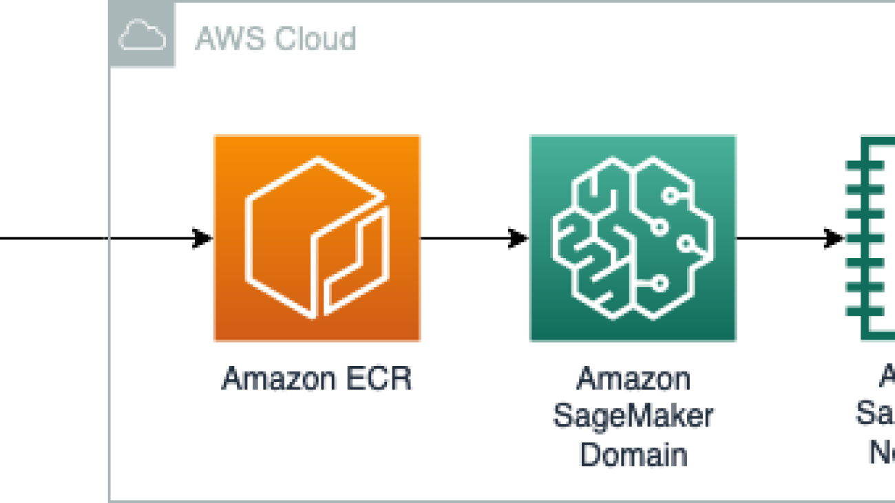
Maira Ladeira Tanke is an ML Specialist Solutions Architect at AWS. With a background in data science, she has 9 years of experience architecting and building ML applications with customers across industries. As a technical lead, she helps customers accelerate their achievement of business value through emerging technologies and innovative solutions. In her free time, Maira enjoys traveling and spending time with her family someplace warm.

Clay Elmore is an AI/ML Specialist Solutions Architect at AWS. After spending many hours in a materials research lab, his background in chemical engineering was quickly left behind to pursue his interest in machine learning. He has worked on ML applications in many different industries ranging from energy trading to hospitality marketing. Clay has a special interest in bringing software development practices to ML and guiding customers towards repeatable, scalable solutions by using these principles. In his spare time, Clay enjoys skiing, solving Rubik’s cubes, reading, and cooking.

Shelbee Eigenbrode is a Principal AI and Machine Learning Specialist Solutions Architect at AWS. She has been in technology for 24 years spanning multiple industries, technologies, and roles. She is currently focusing on combining her DevOps and ML background into the domain of MLOps to help customers deliver and manage ML workloads at scale. With over 35 patents granted across various technology domains, she has a passion for continuous innovation and using data to drive business outcomes. Shelbee is a co-creator and instructor of the Practical Data Science specialization on Coursera. She is also the Co-Director of Women In Big Data (WiBD), Denver chapter. In her spare time, she likes to spend time with her family, friends, and overactive dogs.

Qiyun Zhao is a Senior Software Development Engineer with the Amazon SageMaker Inference Platform team. He is the lead developer of the deployment guardrails and shadow deployments, and he focuses on helping customers to manage ML workloads and deployments at scale with high availability. He also works on platform architecture evolutions for fast and secure ML jobs deployment and running ML online experiments at ease. In his spare time, he enjoys reading, gaming, and traveling.

Read More