New tool lets customers build, train, and deploy machine learning models using only natural language.Read More
Implement human-in-the-loop confirmation with Amazon Bedrock Agents
Agents are revolutionizing how businesses automate complex workflows and decision-making processes. Amazon Bedrock Agents helps you accelerate generative AI application development by orchestrating multi-step tasks. Agents use the reasoning capability of foundation models (FMs) to break down user-requested tasks into multiple steps. In addition, they use the developer-provided instruction to create an orchestration plan and then carry out the plan by invoking company APIs and accessing knowledge bases using Retrieval Augmented Generation (RAG) to provide an answer to the user’s request.
Building intelligent autonomous agents that effectively handle user queries requires careful planning and robust safeguards. Although FMs continue to improve, they can still produce incorrect outputs, and because agents are complex systems, errors can occur at multiple stages. For example, an agent might select the wrong tool or use correct tools with incorrect parameters. Although Amazon Bedrock agents can self-correct through their reasoning and action (ReAct) strategy, repeated tool execution might be acceptable for non-critical tasks but risky for business-critical operations, such as database modifications.
In these sensitive scenarios, human-in-the-loop (HITL) interaction is essential for successful AI agent deployments, encompassing multiple critical touchpoints between humans and automated systems. HITL can take many forms, from end-users approving actions and providing feedback, to subject matter experts reviewing responses offline and agents working alongside customer service representatives. The common thread is maintaining human oversight and using human intelligence to improve agent performance. This human involvement helps establish ground truth, validates agent responses before they go live, and enables continuous learning through feedback loops.
In this post, we focus specifically on enabling end-users to approve actions and provide feedback using built-in Amazon Bedrock Agents features, specifically HITL patterns for providing safe and effective agent operations. We explore the patterns available using a Human Resources (HR) agent example that helps employees requesting time off. You can recreate the example manually or using the AWS Cloud Development Kit (AWS CDK) by following our GitHub repository. We show you what these methods look like from an application developer’s perspective while providing you with the overall idea behind the concepts. For the post, we apply user confirmation and return of control on Amazon Bedrock to achieve the human confirmation.
Amazon Bedrock Agents frameworks for human-in-the-loop confirmation
When implementing human validation in Amazon Bedrock Agents, developers have two primary frameworks at their disposal: user confirmation and return of control (ROC). These mechanisms, though serving similar oversight purposes, address different validation needs and operate at different levels of the agent’s workflow.
User confirmation provides a straightforward way to pause and validate specific actions before execution. With user confirmation, the developer receives information about the function (or API) and parameters values that an agent wants to use to complete a certain task. The developer can then expose this information to the user in the agentic application to collect a confirmation that the function should be executed before continuing the agent’s orchestration process.
With ROC, the agent provides the developer with the information about the task that it wants to execute and completely relies on the developer to execute the task. In this approach, the developer has the possibility to not only validate the agent’s decision, but also contribute with additional context and modify parameters during the agent’s execution process. ROC also happens to be configured at the action group level, covering multiple actions.
Let’s explore how each framework can be implemented and their specific use cases.
Autonomous agent execution: No human-in-the-loop
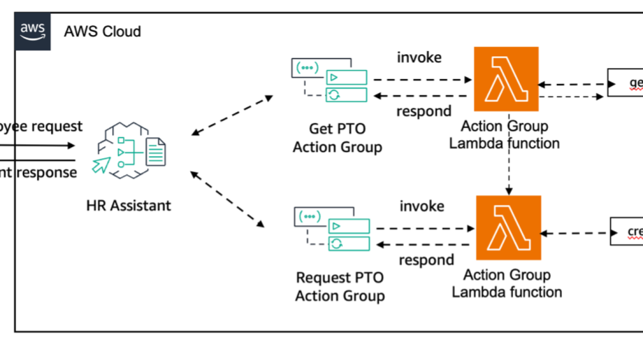
First, let’s demonstrate what a user experience might look like if your application doesn’t have a HITL. For that, let’s consider the following architecture.

In the preceding diagram, the employee interacts with the HR Assistant agent, which then invokes actions that can change important details about the employee’s paid time off (PTO). In this scenario, when an employee requests time off, the agent will automatically request the leave after confirming that enough PTO days are still available for the requesting employee.
The following screenshot shows a sample frontend UI for an Amazon Bedrock agent with functions to retrieve PTOs and request new ones.

In this interaction, the PTO request was submitted with no confirmation from the end-user. What if the user didn’t want to actually submit a request, but only check that it could be done? What if the date they provided was incorrect and had a typo? For any action that changes the state of a user’s PTO, it would provide a better user experience if the system asked for confirmation before actually making those changes.
Simple human validation: User confirmation
When requesting PTO, employees expect to be able to confirm their actions. This minimizes the execution of accidental requests and helps confirm that the agent understood the request and its parameters correctly.
For such scenarios, a Boolean confirmation is already sufficient to continue to execution of the agentic flow. Amazon Bedrock Agents offers an out-of-the-box user confirmation feature that enables developers to incorporate an extra layer of safety and control into their AI-driven workflows. This mechanism strikes a balance between automation and human oversight by making sure that critical actions are validated by users before execution. With user confirmation, developers can decide which tools can be executed automatically and which ones should be first confirmed.
For our example, reading the values for available PTO hours and listing the past PTO requests taken by an employee are non-critical operations that can be executed automatically. However, booking, updating, or canceling a PTO request requires changes on a database and are actions that should be confirmed before execution. Let’s change our agent architecture to include user confirmation, as shown in the following updated diagram.

In the updated architecture, when the employee interacts with the HR Assistant agent and the create_pto_request() action needs to be invoked, the agent will first request user confirmation before execution.
To enable user confirmation, agent developers can use the AWS Management Console, an SDK such as Boto3, or infrastructure as code (IaC) with AWS CloudFormation (see AWS::Bedrock::Agent Function). The user experience with user confirmation will look like the following screenshot.
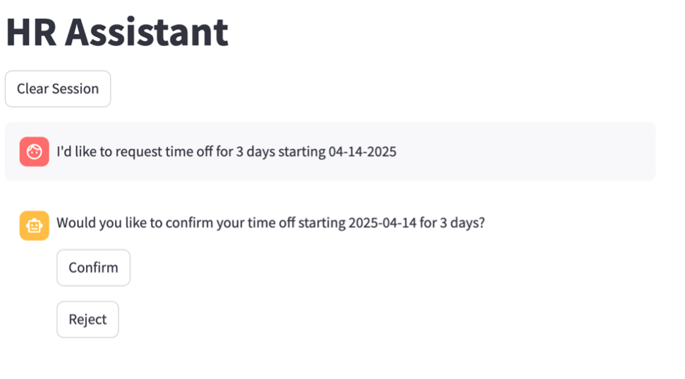
In this interaction, the agent requests a confirmation from the end-user in order to execute. The user can then choose if they want to proceed with the time off request or not. Choosing Confirm will let the agent execute the action based on the parameter displayed.

The following diagram illustrates the workflow for confirming the action.

In this scenario, the developer maps the way the confirmation is displayed to the user in the client-side UI and the agent validates the confirmation state before executing the action.
Customized human input: Return of control
User confirmation provides a simple yes/no validation, but some scenarios require a more nuanced human input. This is where ROC comes into play. ROC allows for a deeper level of human intervention, enabling users to modify parameters or provide additional context before an action is executed.
Let’s consider our HR agent example. When requesting PTO, a common business requirement is for employees to review and potentially edit their requests before submission. This expands upon the simple confirmation use case by allowing users to alter their original input before sending a request to the backend. Amazon Bedrock Agents offers an out-of-the-box solution to effectively parse user input and send it back in a structured format using ROC.
To implement ROC, we need to modify our agent architecture slightly, as shown in the following diagram.

In this architecture, ROC is implemented at the action group level. When an employee interacts with the HR Assistant agent, the system requires explicit confirmation of all function parameters under the “Request PTO Action Group” before executing actions within the action group.
With ROC, the user experience becomes more interactive and flexible. The following screenshot shows an example with our HR agent application.

Instead of executing the action automatically or just having a confirm/deny option, users are presented with a form to edit their intentions directly before processing. In this case, our user can realize they accidentally started their time off request on a Sunday and can edit this information before submission.
After the user reviews and potentially modifies the request, they can approve the parameters.

When implementing ROC, it’s crucial to understand that parameter validation occurs at two distinct points. The agent performs initial validation before returning control to the user (for example, checking available PTO balance), and the final execution relies on the application’s API validation layer.
For instance, if a user initially requests 3 days of PTO, the agent validates against their 5-day balance and returns control. However, if the user modifies the request to 100 days during ROC, the final validation and enforcement happen at the API level, not through the agent. This differs from confirmation flows where the agent directly executes API calls. In ROC, the agent’s role is to facilitate the interaction and return API responses, and the application maintains ultimate control over parameter validation and execution.
The core difference in the ROC approach is that the responsibility of processing the time off request is now handled by the application itself instead of being automatically handled by the agent. This allows for more complex workflows and greater human oversight.
To better understand the flow of information in a ROC scenario, let’s examine the following sequence diagram.

In this workflow, the agent prepares the action but doesn’t execute it. Instead, it returns control to the application, which then presents the editable information to the user. After the user reviews and potentially modifies the request, the application is responsible for executing the action with the final, user-approved parameters.
This approach provides several benefits:
- Enhanced accuracy – Users can correct misunderstandings or errors in the agent’s interpretation of their request
- Flexibility – It allows for last-minute changes or additions to the request
- User empowerment – It gives users more control over the final action, increasing trust in the system
- Compliance – In regulated industries, this level of human oversight can be crucial for adhering to legal or policy requirements
Implementing ROC requires more development effort compared to user confirmation, because it involves creating UIs for editing and handling the execution of actions within the application. However, for scenarios where precision and user control are paramount, the additional complexity is often justified.
Conclusion
In this post, we explored two primary frameworks for implementing human validation in Amazon Bedrock Agents: user confirmation and return of control. Although these mechanisms serve similar oversight purposes, they address different validation needs and operate at distinct levels of the agent’s workflow. User confirmation provides a straightforward Boolean validation, allowing users to approve or reject specific actions before execution. This method is ideal for scenarios where a simple yes/no decision is sufficient to promote safety and accuracy.
ROC offers a more nuanced approach, enabling users to modify parameters and provide additional context before action execution. This framework is particularly useful in complex scenarios, where changing of the agent’s decisions is necessary.
Both methods contribute to a robust HITL approach, providing an essential layer of human validation to the agentic application.
User confirmation and ROC are just two aspects of the broader HITL paradigm in AI agent deployments. In future posts, we will address other crucial use cases for HITL interactions with agents.
To get started creating your own agentic application with HITL validation, we encourage you to explore the HR example discussed in this post. You can find the complete code and implementation details in our GitHub repository.
About the Authors
 Clement Perrot is a Senior Solutions Architect and AI/ML Specialist at AWS, where he helps early-stage startups build and implement AI solutions on the AWS platform. In his role, he architects large-scale GenAI solutions, guides startups in implementing LLM-based applications, and drives the technical adoption of AWS GenAI services globally. He collaborates with field teams on complex customer implementations and authors technical content to enable AWS GenAI adoption. Prior to AWS, Clement founded two successful startups that were acquired, and was recognized with an Inc 30 under 30 award.
 Ryan Sachs is a Solutions Architect at AWS, specializing in GenAI application development. Ryan has a background in developing web/mobile applications at companies large and small through REST APIs. Ryan helps early-stage companies solve their business problems by integrating Generative AI technologies into their existing architectures.
 Maira Ladeira Tanke is a Tech Lead for Agentic workloads in Amazon Bedrock at AWS, where she enables customers on their journey todevelop autonomous AI systems. With over 10 years of experience in AI/ML. At AWS, Maira partners with enterprise customers to accelerate the adoption of agentic applications using Amazon Bedrock, helping organizations harness the power of foundation models to drive innovation and business transformation. In her free time, Maira enjoys traveling, playing with her cat, and spending time with her family someplace warm.
 Mark Roy is a Principal Machine Learning Architect for AWS, helping customers design and build AI/ML solutions. Mark’s work covers a wide range of ML use cases, with a primary interest in computer vision, deep learning, and scaling ML across the enterprise. He has helped companies in many industries, including insurance, financial services, media and entertainment, healthcare, utilities, and manufacturing. Mark holds six AWS Certifications, including the ML Specialty Certification. Prior to joining AWS, Mark was an architect, developer, and technology leader for over 25 years, including 19 years in financial services.
Boost team productivity with Amazon Q Business Insights
Employee productivity is a critical factor in maintaining a competitive advantage. Amazon Q Business offers a unique opportunity to enhance workforce efficiency by providing AI-powered assistance that can significantly reduce the time spent searching for information, generating content, and completing routine tasks. Amazon Q Business is a fully managed, generative AI-powered assistant that lets you build interactive chat applications using your enterprise data, generating answers based on your data or large language model (LLM) knowledge. At the core of this capability are native data source connectors that seamlessly integrate and index content from multiple data sources like Salesforce, Jira, and SharePoint into a unified index.
Key benefits for organizations include:
- Simplified deployment and management – Provides a ready-to-use web experience with no machine learning (ML) infrastructure to maintain or manage
- Access controls – Makes sure users only access content they have permission to view
- Accurate query responses – Delivers precise answers with source citations, analyzing enterprise data
- Privacy and control – Offers comprehensive guardrails and fine-grained access controls
- Broad connectivity – Supports over 45 native data source connectors (at the time of writing), and provides the ability to create custom connectors
Data privacy and the protection of intellectual property are paramount concerns for most organizations. At Amazon, “Security is Job Zero,” which is why Amazon Q Business is designed with these critical considerations in mind. Your data is not used for training purposes, and the answers provided by Amazon Q Business are based solely on the data users have access to. This makes sure that enterprises can quickly find answers to questions, provide summaries, generate content, and complete tasks across various use cases with complete confidence in data security. Amazon Q Business supports encryption in transit and at rest, allowing end-users to use their own encryption keys for added security. This robust security framework enables end-users to receive immediate, permissions-aware responses from enterprise data sources with citations, helping streamline workplace tasks while maintaining the highest standards of data privacy and protection.
Amazon Q Business Insights provides administrators with details about the utilization and effectiveness of their AI-powered applications. By monitoring utilization metrics, organizations can quantify the actual productivity gains achieved with Amazon Q Business. Understanding how employees interact with and use Amazon Q Business becomes crucial for measuring its return on investment and identifying potential areas for further optimization. Tracking metrics such as time saved and number of queries resolved can provide tangible evidence of the service’s impact on overall workplace productivity. It’s essential for admins to periodically review these metrics to understand how users are engaging with Amazon Q Business and identify potential areas of improvement.
The dashboard enables administrators to track user interactions, including the helpfulness of generated answers through user ratings. By visualizing this feedback, admins can pinpoint instances where users aren’t receiving satisfactory responses. With Amazon Q Business Insights, administrators can diagnose potential issues such as unclear user prompts, misconfigured topics and guardrails, insufficient metadata boosters, or inadequate data source configurations. This comprehensive analytics approach empowers organizations to continuously refine their Amazon Q Business implementation, making sure users receive the most relevant and helpful AI-assisted support.
In this post, we explore Amazon Q Business Insights capabilities and its importance for organizations. We begin with an overview of the available metrics and how they can be used for measuring user engagement and system effectiveness. Then we provide instructions for accessing and navigating this dashboard. Finally, we demonstrate how to integrate Amazon Q Business logs with Amazon CloudWatch, enabling deeper insights into user interaction patterns and identifying areas for improvement. This integration can empower administrators to make data-driven decisions for optimizing their Amazon Q Business implementations and maximizing return on investment (ROI).
Amazon Q Business and Amazon Q Apps analytics dashboards
In this section, we discuss the Amazon Q Business and Amazon Q Apps analytics dashboards.
Overview of key metrics
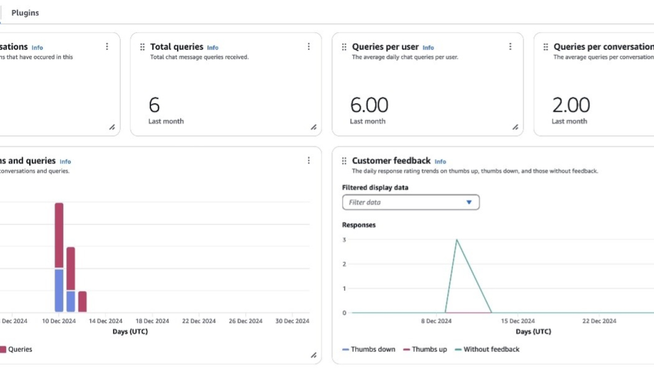
Amazon Q Business Insights (see the following screenshot) offers a comprehensive set of metrics that provide valuable insights into user engagement and system performance. Key metrics include Total queries and Total conversations, which give an overall picture of system usage. More specific metrics such as Queries per conversation and Queries per user offer deeper insights into user interaction patterns and the complexity of inquiries. The Number of conversations and Number of queries metrics help administrators track adoption and usage trends over time.
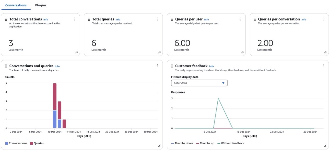
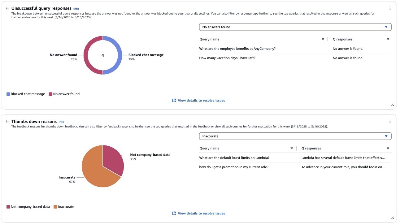
The dashboard also provides critical information on system effectiveness through metrics like Unsuccessful query responses and Thumbs down reasons (see the following screenshot), which highlight areas where the AI assistant might be struggling to provide adequate answers. This is complemented by the end-user feedback metric, which includes user ratings and response effectiveness reasons. These metrics are particularly valuable for identifying specific issues users are encountering and areas where the system needs improvement.
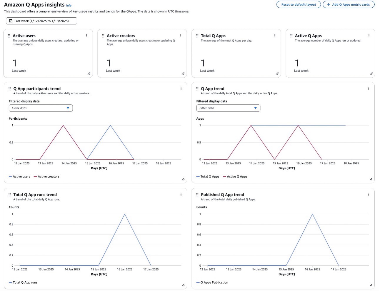
Complementing the main dashboard, Amazon Q Business provides a dedicated analytics dashboard for Amazon Q Apps that offers detailed insights into application creation, usage, and adoption patterns. The dashboard tracks user engagement through metrics like:
- Active users (average unique daily users interacting with Amazon Q Apps)
- Active creators (average unique daily users creating or updating Amazon Q Apps)
Application metrics include:
- Total Q Apps (average daily total)
- Active Q Apps (average number of applications run or updated daily)
These metrics help provide a clear picture of application utilization.
The dashboard also features several trend analyses that help administrators understand usage patterns over time:
- Q App participants trend shows the relationship between daily active users and creators
- Q App trend displays the correlation between total applications created and active applications
- Total Q App runs trend and Published Q App trend track daily execution rates and publication patterns, respectively
These metrics enable administrators to evaluate the performance and adoption of Amazon Q Apps within their organization, helping identify successful implementation patterns and areas needing attention.
These comprehensive metrics are crucial for organizations to optimize their Amazon Q Business implementation and maximize ROI. By analyzing trends in Total queries, Total conversations, and user-specific metrics, administrators can gauge adoption rates and identify potential areas for user training or system improvements. The Unsuccessful query responses and Customer feedback metrics help pinpoint gaps in the knowledge base or areas where the system struggles to provide satisfactory answers. By using these metrics, organizations can make data-driven decisions to enhance the effectiveness of their AI-powered assistant, ultimately leading to improved productivity and user experience across various use cases within the enterprise.
How to access Amazon Q Business Insights dashboards
As an Amazon Q admin, you can view the dashboards on the Amazon Q Business console. You can view the metrics in these dashboards over different pre-selected time intervals. They are available at no additional charge in AWS Regions where the Amazon Q Business service is offered.
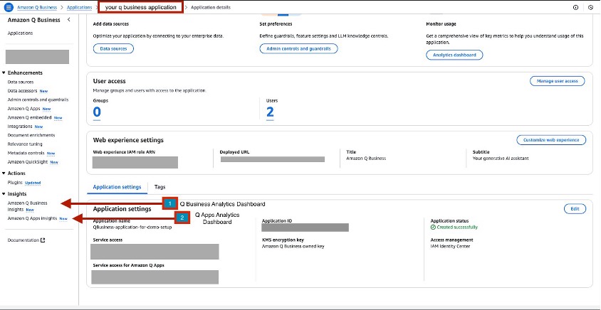
To view these dashboards on the Amazon Q Business console, you choose your application environment and navigate to the Insights page. For more details, see Viewing the analytics dashboards.
The following screenshot illustrates how to access the dashboards for Amazon Q Business applications and Amazon Q Apps Insights.
Monitor Amazon Q Business user conversations
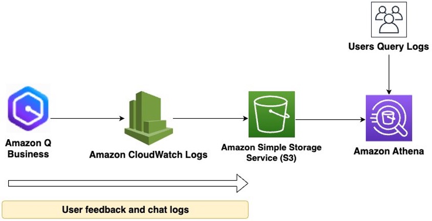
In addition to Amazon Q Business and Amazon Q Apps dashboards, you can use Amazon CloudWatch Logs to deliver user conversations and response feedback in Amazon Q Business for you to analyze. These logs can be delivered to multiple destinations, such as CloudWatch, Amazon Simple Storage Service (Amazon S3), or Amazon Data Firehose.
The following diagram depicts the flow of user conversation and feedback responses from Amazon Q Business to Amazon S3. These logs are then queryable using Amazon Athena.
Prerequisites
To set up CloudWatch Logs for Amazon Q Business, make sure you have the appropriate permissions for the intended destination. Refer to Monitoring Amazon Q Business and Q Apps for more details.
Set up log delivery with CloudWatch as a destination
Complete the following steps to set up log delivery with CloudWatch as the destination:
- Open the Amazon Q Business console and sign in to your account.
- In Applications, choose the name of your application environment.
- In the navigation pane, choose Enhancements and choose Admin Controls and Guardrails.
- In Log delivery, choose Add and select the option To Amazon CloudWatch Logs.
- For Destination log group, enter the log group where the logs will be stored.
Log groups prefixed with /aws/vendedlogs/ will be created automatically. Other log groups must be created prior to setting up a log delivery.
- To filter out sensitive or personally identifiable information (PII), choose Additional settings – optional and specify the fields to be logged, output format, and field delimiter.
If you want the users’ email recorded in your logs, it must be added explicitly as a field in Additional settings.
- Choose Add.
- Choose Enable logging to start streaming conversation and feedback data to your logging destination.
Set up log delivery with Amazon S3 as a destination
To use Amazon S3 as a log destination, you will need an S3 bucket and grant Amazon Q Business the appropriate permissions to write your logs to Amazon S3.
- Open the Amazon Q Business console and sign in to your account.
- In Applications, choose the name of your application environment.
- In the navigation pane, choose Enhancements and choose Admin Controls and Guardrails.
- In Log delivery, choose Add and select the option To Amazon S3
- For Destination S3 bucket, enter your bucket.
- To filter out sensitive or PII data, choose Additional settings – optional and specify the fields to be logged, output format, and field delimiter.
If you want the users’ email recorded in your logs, it must be added explicitly as a field in Additional settings.
- Choose Add.
- Choose Enable logging to start streaming conversation and feedback data to your logging destination.
The logs are delivered to your S3 bucket with the following prefix: AWSLogs/<your-aws-account-id>/AmazonQBusinessLogs/<your-aws-region>/<your-q-business-application--id>/year/month/day/hour/ The placeholders will be replaced with your AWS account, Region, and Amazon Q Business application identifier, respectively.
Set up Data Firehose as a log destination
Amazon Q Business application event logs can also be streamed to Data Firehose as a destination. This can be used for real-time observability. We have excluded setup instructions for brevity.
To use Data Firehose as a log destination, you need to create a Firehose delivery stream (with Direct PUT enabled) and grant Amazon Q Business the appropriate permissions to write your logs to Data Firehose. For example AWS Identity and Access Management (IAM) policies with the required permissions for your specific logging destination, see Enable logging from AWS services.
Protecting sensitive data
You can prevent an AWS console user or group of users from viewing specific CloudWatch log groups, S3 buckets, or Firehose streams by applying specific deny statements in their IAM policies. AWS follows an explicit deny overrides allow model, meaning that if you explicitly deny an action, it will take precedence over allow statements. For more information, see Policy evaluation logic.
Real-world use cases
This section outlines several key use cases for Amazon Q Business Insights, demonstrating how you can use Amazon Q Business operational data to improve your operational posture to help Amazon Q Business meet your needs.
Measure ROI using Amazon Q Business Insights
The dashboards offered by Amazon Q Business Insights provide powerful metrics that help organizations quantify their ROI. Consider this common scenario: traditionally, employees spend countless hours searching through siloed documents, knowledge bases, and various repositories to find answers to their questions. This time-consuming process not only impacts productivity but also leads to significant operational costs. With the dashboards provided by Amazon Q Business Insights, administrators can now measure the actual impact of their investment by tracking key metrics such as total questions answered, total conversations, active users, and positive feedback rates. For instance, if an organization knows that it previously took employees an average of 3 minutes to find an answer in their documentation, and with Amazon Q Business this time is reduced to 20 seconds, they can calculate the time savings per query (2 minutes and 40 seconds). When the dashboard shows 1,000 successful queries per week, this translates to approximately 44 hours of productivity gained—time that employees can now dedicate to higher-value tasks. Organizations can then translate these productivity gains into tangible cost savings based on their specific business metrics.
Furthermore, the dashboard’s positive feedback rate metric helps validate the quality and accuracy of responses, making sure employees aren’t just getting answers, but reliable ones that help them do their jobs effectively. By analyzing these metrics over time—whether it’s over 24 hours, 7 days, or 30 days—organizations can demonstrate how Amazon Q Business is transforming their knowledge management approach from a fragmented, time-intensive process to an efficient, centralized system. This data-driven approach to measuring ROI not only justifies the investment but also helps identify areas where the service can be optimized for even greater returns.
Organizations looking to quantify financial benefits can develop their own ROI calculators tailored to their specific needs. By combining Amazon Q Business Insights metrics with their internal business variables, teams can create customized ROI models that reflect their unique operational context. Several reference calculators are publicly available online, ranging from basic templates to more sophisticated models, which can serve as a starting point for organizations to build their own ROI analysis tools. This approach enables leadership teams to demonstrate the tangible financial benefits of their Amazon Q Business investment and make data-driven decisions about scaling their implementation, based on their organization’s specific metrics and success criteria.
Enforce financial services compliance with Amazon Q Business analytics
Maintaining regulatory compliance while enabling productivity is a delicate balance. As organizations adopt AI-powered tools like Amazon Q Business, it’s crucial to implement proper controls and monitoring. Let’s explore how a financial services organization can use Amazon Q Business Insights capabilities and logging features to maintain compliance and protect against policy violations.
Consider this scenario: A large investment firm has adopted Amazon Q Business to help their financial advisors quickly access client information, investment policies, and regulatory documentation. However, the compliance team needs to make sure the system isn’t being used to circumvent trading restrictions, particularly around day trading activities that could violate SEC regulations and company policies.
Identify policy violations through Amazon Q Business logs
When the compliance team enables log delivery to CloudWatch with the user_email field selected, Amazon Q Business begins sending detailed event logs to CloudWatch. These logs are separated into two CloudWatch log streams:
- QBusiness/Chat/Message – Contains user interactions
- QBusiness/Chat/Feedback – Contains user feedback on responses
For example, the compliance team monitoring the logs might spot this concerning chat from Amazon Q Business:
The compliance team can automate this search by creating an alarm on CloudWatch Metrics Insights queries in CloudWatch.
Implement preventative controls
Upon identifying these attempts, the Amazon Q Business admin can implement several immediate controls within Amazon Q Business:
- Configure blocked phrases to make sure chat responses don’t include these words
- Configure topic-level controls to configure rules to customize how Amazon Q Business should respond when a chat message matches a special topic
The following screenshot depicts configuring topic-level controls for the phrase “day trading.”
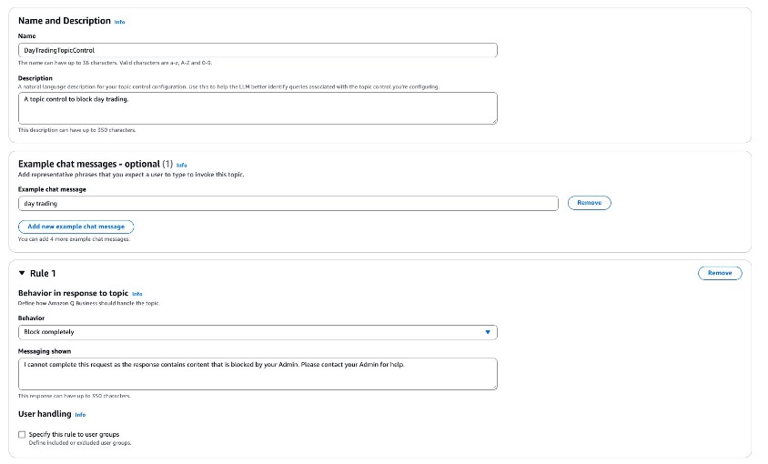
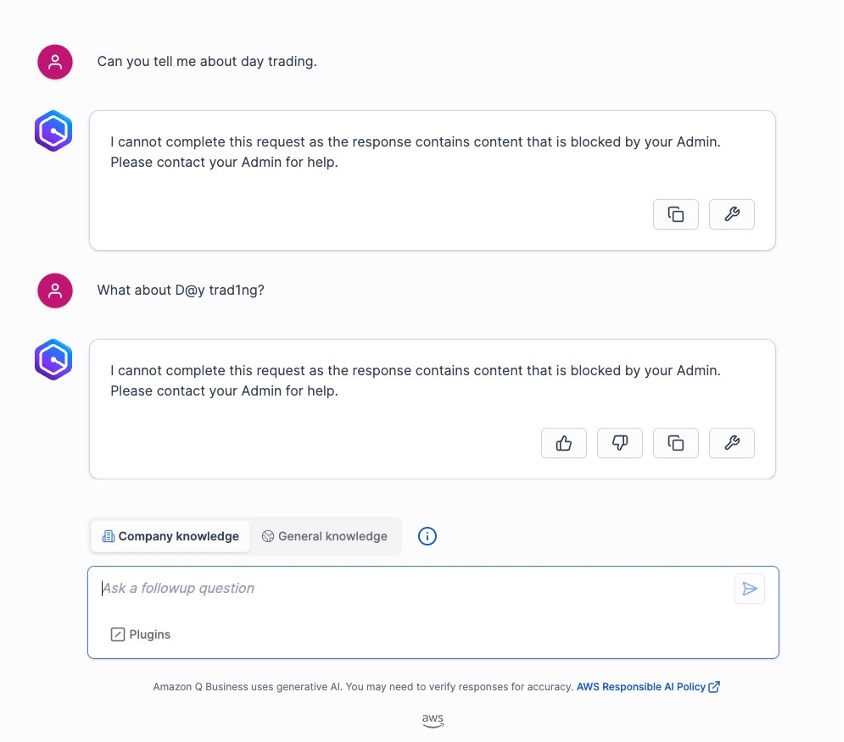
Using the previous topic-level controls, different variations of the phrase “day trading” will be blocked. The following screenshot represents a user entering variations of the phrase “day trading” and how Amazon Q Business blocks that phrase due to the topic-level control for the phrase.
By implementing monitoring and configuring guardrails, the investment firm can maintain its regulatory compliance while still allowing legitimate use of Amazon Q Business for approved activities. The combination of real-time monitoring through logs and preventive guardrails creates a robust defense against potential violations while maintaining detailed audit trails for regulatory requirements.
Analyze user feedback through the Amazon Q Business Insights dashboard
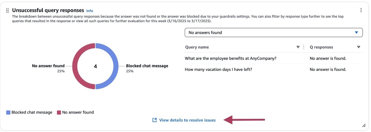
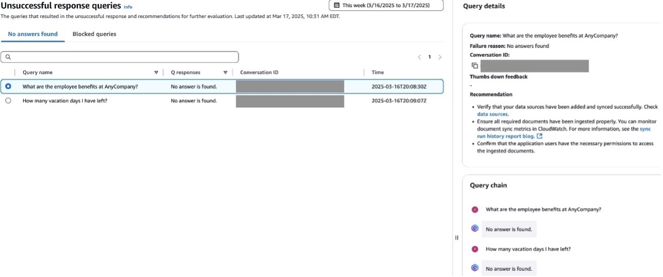
After log delivery has been set up, administrators can use the Amazon Q Business Insights dashboard to get a comprehensive view of user feedback. This dashboard provides valuable data about user experience and areas needing improvement through two key metric cards: Unsuccessful query responses and Thumbs down reasons. The Thumbs down reasons chart offers a detailed breakdown of user feedback, displaying the distribution and frequency of specific reasons why users found responses unhelpful. This granular feedback helps administrators identify patterns in user feedback, whether it’s due to incomplete information, inaccurate responses, or other factors.
Similarly, the Unsuccessful query responses chart distinguishes between queries that failed because answers weren’t found in the knowledge base vs. those blocked by guardrail settings. Both metrics allow administrators to drill down into specific queries through filtering options and detailed views, enabling them to investigate and address issues systematically. This feedback loop is crucial for continuous improvement, helping organizations refine their content, adjust guardrails, and enhance the overall effectiveness of their Amazon Q Business implementation.
To view a breakdown of unsuccessful query responses, follow these steps:
- Select your application on the Amazon Q Business console.
- Select Amazon Q Business insights under Insights.
- Go to the Unsuccessful query responses metrics card and choose View details to resolve issues.
A new page will open with two tabs: No answers found and Blocked queries.
- You can use these tabs to filter by response type. You can also filter by date using the date filter at the top.
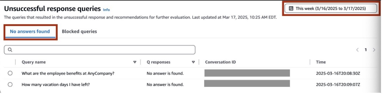
- Choose any of the queries to view the Query chain
This will give you more details and context on the conversation the user had when providing their feedback.
Analyze user feedback through CloudWatch logs
This use case focuses on identifying and analyzing unsatisfactory feedback from specific users in Amazon Q Business. After log delivery is enabled with the user_email field selected, the Amazon Q Business application sends event logs to the previously created CloudWatch log group. User chat interactions and feedback submissions generate events in the QBusiness/Chat/Message and QBusiness/Chat/Feedback log streams, respectively.
For example, consider if a user asks about their vacation policy and no answer is returned. The user can then choose the thumbs down icon and send feedback to the administrator.
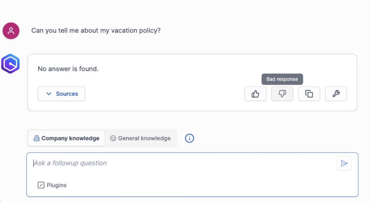
The Send your feedback form provides the user the option to categorize the feedback and provide additional details for the administrator to review.

This feedback will be sent to the QBusiness/Chat/Feedback log stream for the administrator to later analyze. See the following example log entry:
By analyzing queries that result in unsatisfactory responses (thumbs down), administrators can take actions to improve answer quality, accuracy, and security. This feedback can help identify gaps in data sources. Patterns in feedback can indicate topics where users might benefit from extra training or guidance on effectively using Amazon Q Business.
To address issues identified through feedback analysis, administrators can take several actions:
- Configure metadata boosting to prioritize more accurate content in responses for queries that consistently receive negative feedback
- Refine guardrails and chat controls to better align with user expectations and organizational policies
- Develop targeted training or documentation to help users formulate more effective prompts, including prompt engineering techniques
- Analyze user prompts to identify potential risks and reinforce proper data handling practices
By monitoring the chat messages and which users are giving “thumbs up” or “thumbs down” responses for the associated prompts, administrators can gain insights into areas where the system might be underperforming, not meeting user expectations, or not complying with your organization’s security policies.
This use case is applicable to the other log delivery options, such as Amazon S3 and Data Firehose.
Group users getting the most unhelpful answers
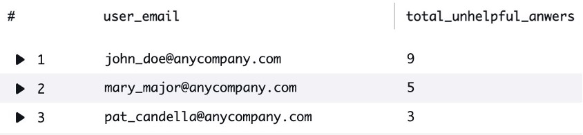
For administrators seeking more granular insights beyond the standard dashboard, CloudWatch Logs Insights offers a powerful tool for deep-dive analysis of Amazon Q Business usage metrics. By using CloudWatch Log Insights, administrators can create custom queries to extract and analyze detailed performance data. For instance, you can generate a sorted list of users experiencing the most unhelpful interactions, such as identifying which employees are consistently receiving unsatisfactory responses. A typical query might reveal patterns like “User A received 9 unhelpful answers in the last 4 weeks, User B received 5 unhelpful answers, and User C received 3 unhelpful answers.” This level of detailed analysis enables organizations to pinpoint specific user groups or departments that might require additional training, data source configuration, or targeted support to improve their Amazon Q Business experience.
To get these kinds of insights, complete the following steps:
- To obtain the Amazon Q Business application ID, open the Amazon Q Business console, open the specific application, and note the application ID on the Application settings
This unique identifier will be used to filter log groups in CloudWatch Logs Insights.
- On the CloudWatch console, choose Logs Insights under Logs in the navigation pane.

- Under Selection criteria, enter the application ID you previously copied. Choose the log group that follows the pattern
/aws/vendedlogs/qbusiness/application/EVENT_LOGS/<your application id>.
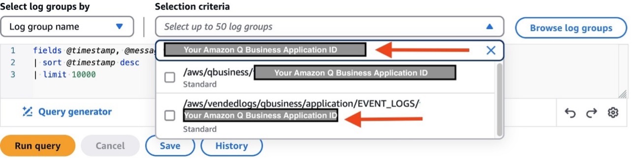
- For the data time range, select the range you want to use. In our case, we are using the last 4 weeks and so we choose Custom, then we specify 4 Weeks.
- Replace the default query in the editor with this one:
We use the condition NOT_USEFUL because we want to list users getting unhelpful answers. To get a list of users who received helpful answers, change the condition to USEFUL.
- Choose Run query.
With this information, particularly user_email, you can write a new query to analyze the conversation logs where users got unhelpful answers. For example, to list messages where user john_doe gave a thumbs down, replace your query with the following:
filter usefulness = "NOT_USEFUL" and user_email = "john_doe@anycompany.com"
Alternatively, to filter unhelpful answers, you could use the following query:
filter usefulness = "NOT_USEFUL"
The results of these queries can help you better understand the context of the feedback users are providing. As mentioned earlier, it might be possible your guardrails are too restrictive, your application is missing a data source, or maybe your users’ prompts are not clear enough.
Clean up
To make sure you don’t incur ongoing costs, clean up resources by removing log delivery configurations, deleting CloudWatch resources, removing the Amazon Q Business application, and deleting any additional AWS resources created after you’re done experimenting with this functionality.
Conclusion
In this post, we explored several ways to improve your operational posture with Amazon Q Business Insights dashboards, the Amazon Q Apps analytics dashboard, and logging with CloudWatch Logs. By using these tools, organizations can gain valuable insights into user engagement patterns, identify areas for improvement, and make sure their Amazon Q Business implementation aligns with security and compliance requirements.
To learn more about Amazon Q Business key usage metrics, refer to Viewing Amazon Q Business and Q App metrics in analytics dashboards. For a comprehensive review of Amazon Q Business CloudWatch logs, including log query examples, refer to Monitoring Amazon Q Business user conversations with Amazon CloudWatch Logs.
About the Authors
 Guillermo Mansilla is a Senior Solutions Architect based in Orlando, Florida. Guillermo has developed a keen interest in serverless architectures and generative AI applications. Prior to his current role, he gained over a decade of experience working as a software developer. Away from work, Guillermo enjoys participating in chess tournaments at his local chess club, a pursuit that allows him to exercise his analytical skills in a different context.
 Amit Gupta is a Senior Q Business Solutions Architect Solutions Architect at AWS. He is passionate about enabling customers with well-architected generative AI solutions at scale.
 Jed Lechner is a Specialist Solutions Architect at Amazon Web Services specializing in generative AI solutions with Amazon Q Business and Amazon Q Apps. Prior to his current role, he worked as a Software Engineer at AWS and other companies, focusing on sustainability technology, big data analytics, and cloud computing. Outside of work, he enjoys hiking and photography, and capturing nature’s moments through his lens.
 Leo Mentis Raj Selvaraj is a Sr. Specialist Solutions Architect – GenAI at AWS with 4.5 years of experience, currently guiding customers through their GenAI implementation journeys. Previously, he architected data platform and analytics solutions for strategic customers using a comprehensive range of AWS services including storage, compute, databases, serverless, analytics, and ML technologies. Leo also collaborates with internal AWS teams to drive product feature development based on customer feedback, contributing to the evolution of AWS offerings.
Multi-LLM routing strategies for generative AI applications on AWS
Organizations are increasingly using multiple large language models (LLMs) when building generative AI applications. Although an individual LLM can be highly capable, it might not optimally address a wide range of use cases or meet diverse performance requirements. The multi-LLM approach enables organizations to effectively choose the right model for each task, adapt to different domains, and optimize for specific cost, latency, or quality needs. This strategy results in more robust, versatile, and efficient applications that better serve diverse user needs and business objectives.
Deploying a multi-LLM application comes with the challenge of routing each user prompt to an appropriate LLM for the intended task. The routing logic must accurately interpret and map the prompt into one of the pre-defined tasks, and then direct it to the assigned LLM for that task. In this post, we provide an overview of common multi-LLM applications. We then explore strategies for implementing effective multi-LLM routing in these applications, discussing the key factors that influence the selection and implementation of such strategies. Finally, we provide sample implementations that you can use as a starting point for your own multi-LLM routing deployments.
Overview of common multi-LLM applications
The following are some of the common scenarios where you might choose to use a multi-LLM approach in your applications:
- Multiple task types – Many use cases need to handle different task types within the same application. For example, a marketing content creation application might need to perform task types such as text generation, text summarization, sentiment analysis, and information extraction as part of producing high-quality, personalized content. Each distinct task type will likely require a separate LLM, which might also be fine-tuned with custom data.
- Multiple task complexity levels – Some applications are designed to handle a single task type, such as text summarization or question answering. However, they must be able to respond to user queries with varying levels of complexity within the same task type. For example, consider a text summarization AI assistant intended for academic research and literature review. Some user queries might be relatively straightforward, simply asking the application to summarize the core ideas and conclusions from a short article. Such queries could be effectively handled by a simple, lower-cost model. In contrast, more complex questions might require the application to summarize a lengthy dissertation by performing deeper analysis, comparison, and evaluation of the research results. These types of queries would be better addressed by more advanced models with greater reasoning capabilities.
- Multiple task domains – Certain applications need to serve users across multiple domains of expertise. An example is a virtual assistant for enterprise business operations. Such a virtual assistant should support users across various business functions, such as finance, legal, human resources, and operations. To handle this breadth of expertise, the virtual assistant needs to use different LLMs that have been fine-tuned on datasets specific to each respective domain.
- Software-as-a-service (SaaS) applications with tenant tiering – SaaS applications are often architected to provide different pricing and experiences to a spectrum of customer profiles, referred to as tiers. Through the use of different LLMs tailored to each tier, SaaS applications can offer capabilities that align with the varying needs and budgets of their diverse customer base. For instance, consider an AI-driven legal document analysis system designed for businesses of varying sizes, offering two primary subscription tiers: Basic and Pro. The Basic tier would use a smaller, more lightweight LLM well-suited for straightforward tasks, such as performing simple document searches or generating summaries of uncomplicated legal documents. The Pro tier, however, would require a highly customized LLM that has been trained on specific data and terminology, enabling it to assist with intricate tasks like drafting complex legal documents.
Multi-LLM routing strategies
In this section, we explore two main approaches to routing requests to different LLMs: static routing and dynamic routing.
Static routing
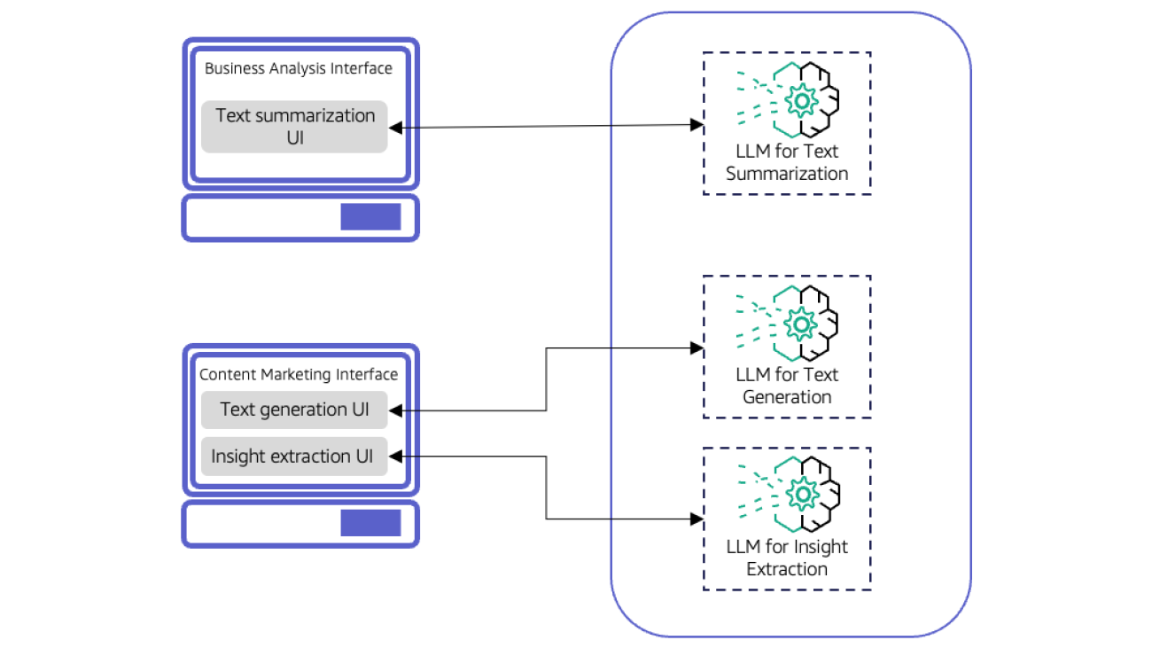
One effective strategy for directing user prompts to appropriate LLMs is to implement distinct UI components within the same interface or separate interfaces tailored to specific tasks. For example, an AI-powered productivity tool for an ecommerce company might feature dedicated interfaces for different roles, such as content marketers and business analysts. The content marketing interface incorporates two main UI components: a text generation module for creating social media posts, emails, and blogs, and an insight extraction module that identifies the most relevant keywords and phrases from customer reviews to improve content strategy. Meanwhile, the business analysis interface would focus on text summarization for analyzing various business documents. This is illustrated in the following figure.

This approach works well for applications where the user experience supports having a distinct UI component for each task. It also allows for a flexible and modular design, where new LLMs can be quickly plugged into or swapped out from a UI component without disrupting the overall system. However, the static nature of this approach implies that the application might not be easily adaptable to evolving user requirements. Adding a new task would necessitate the development of a new UI component in addition to the selection and integration of a new model.
Dynamic routing
In some use cases, such as virtual assistants and multi-purpose chatbots, user prompts usually enter the application through a single UI component. For instance, consider a customer service AI assistant that handles three types of tasks: technical support, billing support, and pre-sale support. Each of these tasks requires its own custom LLM to provide appropriate responses. In this scenario, you need to implement a dynamic routing layer to intercept each incoming request and direct it to the downstream LLM, which is best suited to handle the intended task within that prompt. This is illustrated in the following figure.

In this section, we discuss common approaches for implementing this dynamic routing layer: LLM-assisted routing, semantic routing, and a hybrid approach.
LLM-assisted routing
This approach employs a classifier LLM at the application’s entry point to make routing decisions. The LLM’s ability to comprehend complex patterns and contextual subtleties makes this approach well-suited for applications requiring fine-grained classifications across task types, complexity levels, or domains. However, this method presents trade-offs. Although it offers sophisticated routing capabilities, it introduces additional costs and latency. Furthermore, maintaining the classifier LLM’s relevance as the application evolves can be demanding. Careful model selection, fine-tuning, configuration, and testing might be necessary to balance the impact of latency and cost with the desired classification accuracy.
Semantic routing
This approach uses semantic search as an alternative to using a classifier LLM for prompt classification and routing in multi-LLM systems. Semantic search uses embeddings to represent prompts as numerical vectors. The system then makes routing decisions by measuring the similarity between the user’s prompt embedding and the embeddings for a set of reference prompts, each representing a different task category. The user prompt is then routed to the LLM associated with the task category of the reference prompt that has the closest match.
Although semantic search doesn’t provide explicit classifications like a classifier LLM, it succeeds at identifying broad similarities and can effectively handle variations in a prompt’s wording. This makes it particularly well-suited for applications where routing can be based on coarse-grained classification of prompts, such as task domain classification. It also excels in scenarios with a large number of task categories or when new domains are frequently introduced, because it can quickly accommodate updates by simply adding new prompts to the reference prompt set.
Semantic routing offers several advantages, such as efficiency gained through fast similarity search in vector databases, and scalability to accommodate a large number of task categories and downstream LLMs. However, it also presents some trade-offs. Having adequate coverage for all possible task categories in your reference prompt set is crucial for accurate routing. Additionally, the increased system complexity due to the additional components, such as the vector database and embedding LLM, might impact overall performance and maintainability. Careful design and ongoing maintenance are necessary to address these challenges and fully realize the benefits of the semantic routing approach.
Hybrid approach
In certain scenarios, a hybrid approach combining both techniques might also prove highly effective. For instance, in applications with a large number of task categories or domains, you can use semantic search for initial broad categorization or domain matching, followed by classifier LLMs for more fine-grained classification within those broad categories. This initial filtering allows you to use a simpler, more focused classifier LLM for the final routing decision.
Consider, for instance, a customer service AI assistant handling a diverse range of inquiries. In this context, semantic routing could initially route the user’s prompt to the appropriate department—be it billing, technical support, or sales. After the broad category is established, a dedicated classifier LLM for that specific department takes over. This specialized LLM, which can be trained on nuanced distinctions within its domain, can then determine crucial factors such as task complexity or urgency. Based on this fine-grained analysis, the prompt is then routed to the most appropriate LLM or, when necessary, escalated to a human agent.
This hybrid approach combines the scalability and flexibility of semantic search with the precision and context-awareness of classifier LLMs. The result is a robust, efficient, and highly accurate routing mechanism capable of adapting to the complexities and diverse needs of modern multi-LLM applications.
Implementation of dynamic routing
In this section, we explore different approaches to implementing dynamic routing on AWS, covering both built-in routing features and custom solutions that you can use as a starting point to build your own.
Intelligent prompt routing with Amazon Bedrock
Amazon Bedrock is a fully managed service that makes high-performing LLMs and other foundation models (FMs) from leading AI startups and Amazon available through an API, so you can choose from a wide range of FMs to find the model that is best suited for your use case. With the Amazon Bedrock serverless experience, you can get started quickly, privately customize FMs with your own data, and integrate and deploy them into your applications using AWS tools without having to manage infrastructure.
If you’re building applications with Amazon Bedrock LLMs and need a fully managed solution with straightforward routing capabilities, Amazon Bedrock Intelligent Prompt Routing offers an efficient way to implement dynamic routing. This feature of Amazon Bedrock provides a single serverless endpoint for efficiently routing requests between different LLMs within the same model family. It uses advanced prompt matching and model understanding techniques to predict the performance of each model for every request. Amazon Bedrock then dynamically routes each request to the model that it predicts is most likely to give the desired response at the lowest cost. Intelligent Prompt Routing can reduce costs by up to 30% without compromising on accuracy. As of this writing, Amazon Bedrock supports routing within the Anthropic’s Claude and Meta’s Llama model families. For example, Amazon Bedrock can intelligently route requests between Anthropic’s Claude 3.5 Sonnet and Claude 3 Haiku depending on the complexity of the prompt, as illustrated the following figure. Similarly, Amazon Bedrock can route requests between Meta’s Llama 3.1 70B and 8B.

This architecture workflow includes the following steps:
- A user submits a question through a web or mobile application.
- Anthropic’s prompt router predicts the performance of each downstream LLM, selecting the model that it predicts will offer the best combination of response quality and cost.
- Amazon Bedrock routes the request to the selected LLM, and returns the response along with information about the model.
For detailed implementation guidelines and examples of Intelligent Prompt Routing on Amazon Bedrock, see Reduce costs and latency with Amazon Bedrock Intelligent Prompt Routing and prompt caching.
Custom prompt routing
If your LLMs are hosted outside Amazon Bedrock, such as on Amazon SageMaker or Amazon Elastic Kubernetes Service (Amazon EKS), or you require routing customization, you will need to develop a custom routing solution.
This section provides sample implementations for both LLM-assisted and semantic routing. We discuss the solution’s mechanics, key design decisions, and how to use it as a foundation for developing your own custom routing solutions. For detailed deployment instructions for each routing solution, refer to the GitHub repo. The provided code in this repo is meant to be used in a development environment. Before migrating any of the provided solutions to production, we recommend following the AWS Well-Architected Framework.
LLM-assisted routing
In this solution, we demonstrate an educational tutor assistant that helps students in two domains of history and math. To implement the routing layer, the application uses the Amazon Titan Text G1 – Express model on Amazon Bedrock to classify the questions based on their topic to either history or math. History questions are routed to a more cost-effective and faster LLM such as Anthropic’s Claude 3 Haiku on Amazon Bedrock. Math questions are handled by a more powerful LLM, such as Anthropic’s Claude 3.5 Sonnet on Amazon Bedrock, which is better suited for complex problem-solving, in-depth explanations, and multi-step reasoning. If the classifier LLM is unsure whether a question belongs to the history or math category, it defaults to classifying it as math.
The architecture of this system is illustrated in the following figure. The use of Amazon Titan and Anthropic models on Amazon Bedrock in this demonstration is optional. You can substitute them with other models deployed on or outside of Amazon Bedrock.

This architecture workflow includes the following steps:
- A user submits a question through a web or mobile application, which forwards the query to Amazon API Gateway.
- When API Gateway receives the request, it triggers an AWS Lambda
- The Lambda function sends the question to the classifier LLM to determine whether it is a history or math question.
- Based on the classifier LLM’s decision, the Lambda function routes the question to the appropriate downstream LLM, which will generate an answer and return it to the user.
Follow the deployment steps in the GitHub repo to create the necessary infrastructure for LLM-assisted routing and run tests to generate responses. The following output shows the response to the question “What year did World War II end?”
The question was correctly classified as a history question, with the classification process taking approximately 0.53 seconds. The question was then routed to and answered by Anthropic’s Claude 3 Haiku, which took around 0.25 seconds. In total, it took about 0.78 seconds to receive the response.
Next, we will ask a math question. The following output shows the response to the question “Solve the quadratic equation: 2x^2 – 5x + 3 = 0.”
The question was correctly classified as a math question, with the classification process taking approximately 0.59 seconds. The question was then correctly routed to and answered by Anthropic’s Claude 3.5 Sonnet, which took around 2.3 seconds. In total, it took about 2.9 seconds to receive the response.
Semantic routing
In this solution, we focus on the same educational tutor assistant use case as in LLM-assisted routing. To implement the routing layer, you first need to create a set of reference prompts that represents the full spectrum of history and math topics you intend to cover. This reference set serves as the foundation for the semantic matching process, enabling the application to correctly categorize incoming queries. As an illustrative example, we’ve provided a sample reference set with five questions for each of the history and math topics. In a real-world implementation, you would likely need a much larger and more diverse set of reference questions to have robust routing performance.
You can use the Amazon Titan Text Embeddings V2 model on Amazon Bedrock to convert the questions in the reference set into embeddings. You can find the code for this conversion in the GitHub repo. These embeddings are then saved as a reference index inside an in-memory FAISS vector store, which is deployed as a Lambda layer.
The architecture of this system is illustrated in the following figure. The use of Amazon Titan and Anthropic models on Amazon Bedrock in this demonstration is optional. You can substitute them with other models deployed on or outside of Amazon Bedrock.

This architecture workflow includes the following steps:
- A user submits a question through a web or mobile application, which forwards the query to API Gateway.
- When API Gateway receives the request, it triggers a Lambda function.
- The Lambda function sends the question to the Amazon Titan Text Embeddings V2 model to convert it to an embedding. It then performs a similarity search on the FAISS index to find the closest matching question in the reference index, and returns the corresponding category label.
- Based on the retrieved category, the Lambda function routes the question to the appropriate downstream LLM, which will generate an answer and return it to the user.
Follow the deployment steps in the GitHub repo to create the necessary infrastructure for semantic routing and run tests to generate responses. The following output shows the response to the question “What year did World War II end?”
The question was correctly classified as a history question and the classification took about 0.1 seconds. The question was then routed and answered by Anthropic’s Claude 3 Haiku, which took about 0.25 seconds, resulting in a total of about 0.36 seconds to get the response back.
Next, we ask a math question. The following output shows the response to the question “Solve the quadratic equation: 2x^2 – 5x + 3 = 0.”
The question was correctly classified as a math question and the classification took about 0.1 seconds. Moreover, the question was correctly routed and answered by Anthropic’s 3.5 Claude Sonnet, which took about 2.7 seconds, resulting in a total of about 2.8 seconds to get the response back.
Additional considerations for custom prompt routing
The provided solutions uses exemplary LLMs for classification in LLM-assisted routing and for text embedding in semantic routing. However, you will likely need to evaluate multiple LLMs to select the LLM that is best suited for your specific use case. Using these LLMs does incur additional cost and latency. Therefore, it’s critical that the benefits of dynamically routing queries to the appropriate LLM can justify the overhead introduced by implementing the custom prompt routing system.
For some use cases, especially those that require specialized domain knowledge, consider fine-tuning the classifier LLM in LLM-assisted routing and the embedding LLM in semantic routing with your own proprietary data. This can increase the quality and accuracy of the classification, leading to better routing decisions.
Additionally, the semantic routing solution used FAISS as an in-memory vector database for similarity search. However, you might need to evaluate alternative vector databases on AWS that better fit your use case in terms of scale, latency, and cost requirements. It will also be important to continuously gather prompts from your users and iterate on the reference prompt set. This will help make sure that it reflects the actual types of questions your users are asking, thereby increasing the accuracy of your similarity search classification over time.
Clean up
To avoid incurring additional costs, clean up the resources you created for LLM-assisted routing and semantic routing by running the following command for each of the respective created stacks:
Cost analysis for custom prompt routing
This section analyzes the implementation cost and potential savings for the two custom prompt routing solutions, using an exemplary traffic scenario for our educational tutor assistant application.
Our calculations are based on the following assumptions:
- The application is deployed in the US East (N. Virginia) AWS Region and receives 50,000 history questions and 50,000 math questions per day.
- For LLM-assisted routing, the classifier LLM processes 150 input tokens and generates 1 output token per question.
- For semantic routing, the embedding LLM processes 150 input tokens per question.
- The answerer LLM processes 150 input tokens and generates 300 output tokens per question.
- Amazon Titan Text G1 – Express model performs question classification in LLM-assisted routing at $0.0002 per 1,000 input tokens, with negligible output costs (1 token per question).
- Amazon Titan Text Embeddings V2 model generates question embedding in semantic routing at $0.00002 per 1,000 input tokens.
- Anthropic’s Claude 3 Haiku handles history questions at $0.00025 per 1,000 input tokens and $0.00125 per 1,000 output tokens.
- Anthropic’s Claude 3.5 Sonnet answers math questions at $0.003 per 1,000 input tokens and $0.015 per 1,000 output tokens.
- The Lambda runtime is 3 seconds per math question and 1 second per history question.
- Lambda uses 1024 MB of memory and 512 MB of ephemeral storage, with API Gateway configured as a REST API.
The following table summarizes the cost of answer generation by LLM for both routing strategies.
| Question Type | Total Input Tokens/Month | Total Output Tokens/Month | Answer Generation Cost/Month |
| History | 225,000,000 | 450,000,000 | $618.75 |
| Math | 225,000,000 | 450,000,000 | $7425 |
The following table summarizes the cost of dynamic routing implementation for both routing strategies.
| LLM-Assisted Routing | Semantic Routing | ||||
| Question Type | Total Input Tokens/Month | Classifier LLM Cost/Month | Lambda + API Gateway Cost/Month | Embedding LLM Cost/Month | Lambda + API Gateway Cost/Month |
| History + Math | 450,000,000 | $90 | $98.9 | $9 | $98.9 |
The first table shows that using Anthropic’s Claude 3 Haiku for history questions costs $618.75 per month, whereas using Anthropic’s Claude 3.5 Sonnet for math questions costs $7,425 per month. This demonstrates that routing questions to the appropriate LLM can achieve significant cost savings compared to using the more expensive model for all of the questions. The second table shows that these savings come with an implementation cost of $188.9/month for LLM-assisted routing and $107.9/month for semantic routing, which are relatively small compared to the potential savings in answer generation costs.
Selecting the right dynamic routing implementation
The decision on which dynamic routing implementation is best suited for your use case largely depends on three key factors: model hosting requirements, cost and operational overhead, and desired level of control over routing logic. The following table outlines these dimensions for Amazon Bedrock Intelligent Prompt Routing and custom prompt routing.
| Design Criteria | Amazon Bedrock Intelligent Prompt Routing | Custom Prompt Routing |
| Model Hosting | Limited to Amazon Bedrock hosted models within the same model family | Flexible: can work with models hosted outside of Amazon Bedrock |
| Operational Management | Fully managed service with built-in optimization | Requires custom implementation and optimization |
| Routing Logic Control | Limited customization, predefined optimization for cost and performance | Full control over routing logic and optimization criteria |
These approaches aren’t mutually exclusive. You can implement hybrid solutions, using Amazon Bedrock Intelligent Prompt Routing for certain workloads while maintaining custom prompt routing for others with LLMs hosted outside Amazon Bedrock or where more control on routing logic is needed.
Conclusion
This post explored multi-LLM strategies in modern AI applications, demonstrating how using multiple LLMs can enhance organizational capabilities across diverse tasks and domains. We examined two primary routing strategies: static routing through using dedicated interfaces and dynamic routing using prompt classification at the application’s point of entry.
For dynamic routing, we covered two custom prompt routing strategies, LLM-assisted and semantic routing, and discussed exemplary implementations for each. These techniques enable customized routing logic for LLMs, regardless of their hosting platform. We also discussed Amazon Bedrock Intelligent Prompt Routing as an alternative implementation for dynamic routing, which optimizes response quality and cost by routing prompts across different LLMs within Amazon Bedrock.
Although these dynamic routing approaches offer powerful capabilities, they require careful consideration of engineering trade-offs, including latency, cost optimization, and system maintenance complexity. By understanding these tradeoffs, along with implementation best practices like model evaluation, cost analysis, and domain fine-tuning, you can architect a multi-LLM routing solution optimized for your application’s needs.
About the Authors
 Nima Seifi is a Senior Solutions Architect at AWS, based in Southern California, where he specializes in SaaS and GenAIOps. He serves as a technical advisor to startups building on AWS. Prior to AWS, he worked as a DevOps architect in the ecommerce industry for over 5 years, following a decade of R&D work in mobile internet technologies. Nima has authored over 20 technical publications and holds 7 US patents. Outside of work, he enjoys reading, watching documentaries, and taking beach walks.
 Manish Chugh is a Principal Solutions Architect at AWS based in San Francisco, CA. He specializes in machine learning and is a generative AI lead for NAMER startups team. His role involves helping AWS customers build scalable, secure, and cost-effective machine learning and generative AI workloads on AWS. He regularly presents at AWS conferences and partner events. Outside of work, he enjoys hiking on East SF Bay trails, road biking, and watching (and playing) cricket.

How iFood built a platform to run hundreds of machine learning models with Amazon SageMaker Inference
Headquartered in São Paulo, Brazil, iFood is a national private company and the leader in food-tech in Latin America, processing millions of orders monthly. iFood has stood out for its strategy of incorporating cutting-edge technology into its operations. With the support of AWS, iFood has developed a robust machine learning (ML) inference infrastructure, using services such as Amazon SageMaker to efficiently create and deploy ML models. This partnership has allowed iFood not only to optimize its internal processes, but also to offer innovative solutions to its delivery partners and restaurants.
iFood’s ML platform comprises a set of tools, processes, and workflows developed with the following objectives:
- Accelerate the development and training of AI/ML models, making them more reliable and reproducible
- Make sure that deploying these models to production is reliable, scalable, and traceable
- Facilitate the testing, monitoring, and evaluation of models in production in a transparent, accessible, and standardized manner

To achieve these objectives, iFood uses SageMaker, which simplifies the training and deployment of models. Additionally, the integration of SageMaker features in iFood’s infrastructure automates critical processes, such as generating training datasets, training models, deploying models to production, and continuously monitoring their performance.
In this post, we show how iFood uses SageMaker to revolutionize its ML operations. By harnessing the power of SageMaker, iFood streamlines the entire ML lifecycle, from model training to deployment. This integration not only simplifies complex processes but also automates critical tasks.
AI inference at iFood
iFood has harnessed the power of a robust AI/ML platform to elevate the customer experience across its diverse touchpoints. Using the cutting edge of AI/ML capabilities, the company has developed a suite of transformative solutions to address a multitude of customer use cases:
- Personalized recommendations – At iFood, AI-powered recommendation models analyze a customer’s past order history, preferences, and contextual factors to suggest the most relevant restaurants and menu items. This personalized approach makes sure customers discover new cuisines and dishes tailored to their tastes, improving satisfaction and driving increased order volumes.
- Intelligent order tracking – iFood’s AI systems track orders in real time, predicting delivery times with a high degree of accuracy. By understanding factors like traffic patterns, restaurant preparation times, and courier locations, the AI can proactively notify customers of their order status and expected arrival, reducing uncertainty and anxiety during the delivery process.
- Automated customer Service – To handle the thousands of daily customer inquiries, iFood has developed an AI-powered chatbot that can quickly resolve common issues and questions. This intelligent virtual agent understands natural language, accesses relevant data, and provides personalized responses, delivering fast and consistent support without overburdening the human customer service team.
- Grocery shopping assistance – Integrating advanced language models, iFood’s app allows customers to simply speak or type their recipe needs or grocery list, and the AI will automatically generate a detailed shopping list. This voice-enabled grocery planning feature saves customers time and effort, enhancing their overall shopping experience.
Through these diverse AI-powered initiatives, iFood is able to anticipate customer needs, streamline key processes, and deliver a consistently exceptional experience—further strengthening its position as the leading food-tech platform in Latin America.
Solution overview
The following diagram illustrates iFood’s legacy architecture, which had separate workflows for data science and engineering teams, creating challenges in efficiently deploying accurate, real-time machine learning models into production systems.

In the past, the data science and engineering teams at iFood operated independently. Data scientists would build models using notebooks, adjust weights, and publish them onto services. Engineering teams would then struggle to integrate these models into production systems. This disconnection between the two teams made it challenging to deploy accurate real-time ML models.
To overcome this challenge, iFood built an internal ML platform that helped bridge this gap. This platform has streamlined the workflow, providing a seamless experience for creating, training, and delivering models for inference. It provides a centralized integration where data scientists could build, train, and deploy models seamlessly from an integrated approach, considering the development workflow of the teams. The interaction with engineering teams could consume these models and integrate them into applications from both an online and offline perspective, enabling a more efficient and streamlined workflow.
By breaking down the barriers between data science and engineering, AWS AI platforms empowered iFood to use the full potential of their data and accelerate the development of AI applications. The automated deployment and scalable inference capabilities provided by SageMaker made sure that models were readily available to power intelligent applications and provide accurate predictions on demand. This centralization of ML services as a product has been a game changer for iFood, allowing them to focus on building high-performing models rather than the intricate details of inference.
One of the core capabilities of iFood’s ML platform is the ability to provide the infrastructure to serve predictions. Several use cases are supported by the inference made available through ML Go!, responsible for deploying SageMaker pipelines and endpoints. The former are used to schedule offline predictions jobs, and the latter are employed to create model services, to be consumed by the application services. The following diagram illustrates iFood’s updated architecture, which incorporates an internal ML platform built to streamline workflows between data science and engineering teams, enabling efficient deployment of machine learning models into production systems.

Integrating model deployment into the service development process was a key initiative to enable data scientists and ML engineers to deploy and maintain those models. The ML platform empowers the building and evolution of ML systems. Several other integrations with other important platforms, like the feature platform and data platform, were delivered to increase the experience for the users as a whole. The process of consuming ML-based decisions was streamlined—but it doesn’t end there. The iFood’s ML platform, ML Go!, is now focusing on new inference capabilities, supported by recent features in which the iFood’s team was responsible for supporting their ideation and development. The following diagram illustrates the final architecture of iFood’s ML platform, showcasing how model deployment is integrated into the service development process, the platform’s connections with feature and data platforms, and its focus on new inference capabilities.

One of the biggest changes is oriented to the creation of one abstraction for connecting with SageMaker Endpoints and Jobs, called ML Go! Gateway, and also, the separation of concerns within the Endpoints, by the use of the Inference Components feature, making the serving faster and more efficient. In this new inference structure, the Endpoints are also managed by the ML Go! CI/CD, leaving for the pipelines, to deal only with model promotions, and not the infrastructure itself. It will reduce the lead time to changes, and change failure ratio over the deployments.
Using SageMaker Inference Model Serving Containers:
One of the key features of modern machine learning platforms is the standardization of machine learning and AI services. By encapsulating models and dependencies as Docker containers, these platforms ensure consistency and portability across different environments and stages of ML. Using SageMaker, data scientists and developers can use pre-built Docker containers, making it straightforward to deploy and manage ML services. As a project progresses, they can spin up new instances and configure them according to their specific requirements. SageMaker provides Docker containers that are designed to work seamlessly with SageMaker. These containers provide a standardized and scalable environment for running ML workloads on SageMaker.
SageMaker provides a set of pre-built containers for popular ML frameworks and algorithms, such as TensorFlow, PyTorch, XGBoost, and many others. These containers are optimized for performance and include all the necessary dependencies and libraries pre-installed, making it straightforward to get started with your ML projects. In addition to the pre-built containers, it provides options to bring your own custom containers to SageMaker, which include your specific ML code, dependencies, and libraries. This can be particularly useful if you’re using a less common framework or have specific requirements that aren’t met by the pre-built containers.
iFood was highly focused on using custom containers for the training and deployment of ML workloads, providing a consistent and reproducible environment for ML experiments, and making it effortless to track and replicate results. The first step in this journey was to standardize the ML custom code, which is actually the piece of code that the data scientists should focus on. Without a notebook, and with BruceML, the way to create the code to train and serve models has changed, to be encapsulated from the start as container images. BruceML was responsible for creating the scaffolding required to seamlessly integrate with the SageMaker platform, allowing the teams to take advantage of its various features, such as hyperparameter tuning, model deployment, and monitoring. By standardizing ML services and using containerization, modern platforms democratize ML, enabling iFood to rapidly build, deploy, and scale intelligent applications.
Automating model deployment and ML system retraining
When running ML models in production, it’s critical to have a robust and automated process for deploying and recalibrating those models across different use cases. This helps make sure the models remain accurate and performant over time. The team at iFood understood this challenge well—not only the model is deployed. Instead, they rely on another concept to keep things running well: ML pipelines.
Using Amazon SageMaker Pipelines, they were able to build a CI/CD system for ML, to deliver automated retraining and model deployment. They also integrated this entire system with the company’s existing CI/CD pipeline, making it efficient and also maintaining good DevOps practices used at iFood. It starts with the ML Go! CI/CD pipeline pushing the latest code artifacts containing the model training and deployment logic. It includes the training process, which uses different containers for implementing the entire pipeline. When training is complete, the inference pipeline can be executed to begin the model deployment. It can be an entirely new model, or the promotion of a new version to increase the performance of an existing one. Every model available for deployment is also secured and registered automatically by ML Go! in Amazon SageMaker Model Registry, providing versioning and tracking capabilities.
The final step depends on the intended inference requirements. For batch prediction use cases, the pipeline creates a SageMaker batch transform job to run large-scale predictions. For real-time inference, the pipeline deploys the model to a SageMaker endpoint, carefully selecting the appropriate container variant and instance type to handle the expected production traffic and latency needs. This end-to-end automation has been a game changer for iFood, allowing them to rapidly iterate on their ML models and deploy updates and recalibrations quickly and confidently across their various use cases. SageMaker Pipelines has provided a streamlined way to orchestrate these complex workflows, making sure model operationalization is efficient and reliable.
Running inference in different SLA formats
iFood uses the inference capabilities of SageMaker to power its intelligent applications and deliver accurate predictions to its customers. By integrating the robust inference options available in SageMaker, iFood has been able to seamlessly deploy ML models and make them available for real-time and batch predictions. For iFood’s online, real-time prediction use cases, the company uses SageMaker hosted endpoints to deploy their models. These endpoints are integrated into iFood’s customer-facing applications, allowing for immediate inference on incoming data from users. SageMaker handles the scaling and management of these endpoints, making sure that iFood’s models are readily available to provide accurate predictions and enhance the user experience.
In addition to real-time predictions, iFood also uses SageMaker batch transform to perform large-scale, asynchronous inference on datasets. This is particularly useful for iFood’s data preprocessing and batch prediction requirements, such as generating recommendations or insights for their restaurant partners. SageMaker batch transform jobs enable iFood to efficiently process vast amounts of data, further enhancing their data-driven decision-making.
Building upon the success of standardization to SageMaker Inference, iFood has been instrumental in partnering with the SageMaker Inference team to build and enhance key AI inference capabilities within the SageMaker platform. Since the early days of ML, iFood has provided the SageMaker Inference team with valuable inputs and expertise, enabling the introduction of several new features and optimizations:
- Cost and performance optimizations for generative AI inference – iFood helped the SageMaker Inference team develop innovative techniques to optimize the use of accelerators, enabling SageMaker Inference to reduce foundation model (FM) deployment costs by 50% on average and latency by 20% on average with inference components. This breakthrough delivers significant cost savings and performance improvements for customers running generative AI workloads on SageMaker.
- Scaling improvements for AI inference – iFood’s expertise in distributed systems and auto scaling has also helped the SageMaker team develop advanced capabilities to better handle the scaling requirements of generative AI models. These improvements reduce auto scaling times by up to 40% and auto scaling detection by six times, making sure that customers can rapidly scale their inference workloads on SageMaker to meet spikes in demand without compromising performance.
- Streamlined generative AI model deployment for inference – Recognizing the need for simplified model deployment, iFood collaborated with AWS to introduce the ability to deploy open source large language models (LLMs) and FMs with just a few clicks. This user-friendly functionality removes the complexity traditionally associated with deploying these advanced models, empowering more customers to harness the power of AI.
- Scale-to-zero for inference endpoints – iFood played a crucial role in collaborating with SageMaker Inference to develop and launch the scale-to-zero feature for SageMaker inference endpoints. This innovative capability allows inference endpoints to automatically shut down when not in use and rapidly spin up on demand when new requests arrive. This feature is particularly beneficial for dev/test environments, low-traffic applications, and inference use cases with varying inference demands, because it eliminates idle resource costs while maintaining the ability to quickly serve requests when needed. The scale-to-zero functionality represents a major advancement in cost-efficiency for AI inference, making it more accessible and economically viable for a wider range of use cases.
- Packaging AI model inference more efficiently – To further simplify the AI model lifecycle, iFood worked with AWS to enhance SageMaker’s capabilities for packaging LLMs and models for deployment. These improvements make it straightforward to prepare and deploy these AI models, accelerating their adoption and integration.
- Multi-model endpoints for GPU – iFood collaborated with the SageMaker Inference team to launch multi-model endpoints for GPU-based instances. This enhancement allows you to deploy multiple AI models on a single GPU-enabled endpoint, significantly improving resource utilization and cost-efficiency. By taking advantage of iFood’s expertise in GPU optimization and model serving, SageMaker now offers a solution that can dynamically load and unload models on GPUs, reducing infrastructure costs by up to 75% for customers with multiple models and varying traffic patterns.
- Asynchronous inference – Recognizing the need for handling long-running inference requests, the team at iFood worked closely with the SageMaker Inference team to develop and launch Asynchronous Inference in SageMaker. This feature enables you to process large payloads or time-consuming inference requests without the constraints of real-time API calls. iFood’s experience with large-scale distributed systems helped shape this solution, which now allows for better management of resource-intensive inference tasks, and the ability to handle inference requests that might take several minutes to complete. This capability has opened up new use cases for AI inference, particularly in industries dealing with complex data processing tasks such as genomics, video analysis, and financial modeling.
By closely partnering with the SageMaker Inference team, iFood has played a pivotal role in driving the rapid evolution of AI inference and generative AI inference capabilities in SageMaker. The features and optimizations introduced through this collaboration are empowering AWS customers to unlock the transformative potential of inference with greater ease, cost-effectiveness, and performance.
“At iFood, we were at the forefront of adopting transformative machine learning and AI technologies, and our partnership with the SageMaker Inference product team has been instrumental in shaping the future of AI applications. Together, we’ve developed strategies to efficiently manage inference workloads, allowing us to run models with speed and price-performance. The lessons we’ve learned supported us in the creation of our internal platform, which can serve as a blueprint for other organizations looking to harness the power of AI inference. We believe the features we have built in collaboration will broadly help other enterprises who run inference workloads on SageMaker, unlocking new frontiers of innovation and business transformation, by solving recurring and important problems in the universe of machine learning engineering.”
– says Daniel Vieira, ML Platform manager at iFood.
Conclusion
Using the capabilities of SageMaker, iFood transformed its approach to ML and AI, unleashing new possibilities for enhancing the customer experience. By building a robust and centralized ML platform, iFood has bridged the gap between its data science and engineering teams, streamlining the model lifecycle from development to deployment. The integration of SageMaker features has enabled iFood to deploy ML models for both real-time and batch-oriented use cases. For real-time, customer-facing applications, iFood uses SageMaker hosted endpoints to provide immediate predictions and enhance the user experience. Additionally, the company uses SageMaker batch transform to efficiently process large datasets and generate insights for its restaurant partners. This flexibility in inference options has been key to iFood’s ability to power a diverse range of intelligent applications.
The automation of deployment and retraining through ML Go!, supported by SageMaker Pipelines and SageMaker Inference, has been a game changer for iFood. This has enabled the company to rapidly iterate on its ML models, deploy updates with confidence, and maintain the ongoing performance and reliability of its intelligent applications. Moreover, iFood’s strategic partnership with the SageMaker Inference team has been instrumental in driving the evolution of AI inference capabilities within the platform. Through this collaboration, iFood has helped shape cost and performance optimizations, scale improvements, and simplify model deployment features—all of which are now benefiting a wider range of AWS customers.
By taking advantage of the capabilities SageMaker offers, iFood has been able to unlock the transformative potential of AI and ML, delivering innovative solutions that enhance the customer experience and strengthen its position as the leading food-tech platform in Latin America. This journey serves as a testament to the power of cloud-based AI infrastructure and the value of strategic partnerships in driving technology-driven business transformation.
By following iFood’s example, you can unlock the full potential of SageMaker for your business, driving innovation and staying ahead in your industry.
About the Authors
 Daniel Vieira is a seasoned Machine Learning Engineering Manager at iFood, with a strong academic background in computer science, holding both a bachelor’s and a master’s degree from the Federal University of Minas Gerais (UFMG). With over a decade of experience in software engineering and platform development, Daniel leads iFood’s ML platform, building a robust, scalable ecosystem that drives impactful ML solutions across the company. In his spare time, Daniel Vieira enjoys music, philosophy, and learning about new things while drinking a good cup of coffee.
 Debora Fanin serves as a Senior Customer Solutions Manager AWS for the Digital Native Business segment in Brazil. In this role, Debora manages customer transformations, creating cloud adoption strategies to support cost-effective, timely deployments. Her responsibilities include designing change management plans, guiding solution-focused decisions, and addressing potential risks to align with customer objectives. Debora’s academic path includes a Master’s degree in Administration at FEI and certifications such as Amazon Solutions Architect Associate and Agile credentials. Her professional history spans IT and project management roles across diverse sectors, where she developed expertise in cloud technologies, data science, and customer relations.
 Saurabh Trikande is a Senior Product Manager for Amazon Bedrock and Amazon SageMaker Inference. He is passionate about working with customers and partners, motivated by the goal of democratizing AI. He focuses on core challenges related to deploying complex AI applications, inference with multi-tenant models, cost optimizations, and making the deployment of generative AI models more accessible. In his spare time, Saurabh enjoys hiking, learning about innovative technologies, following TechCrunch, and spending time with his family.
 Gopi Mudiyala is a Senior Technical Account Manager at AWS. He helps customers in the financial services industry with their operations in AWS. As a machine learning enthusiast, Gopi works to help customers succeed in their ML journey. In his spare time, he likes to play badminton, spend time with family, and travel.
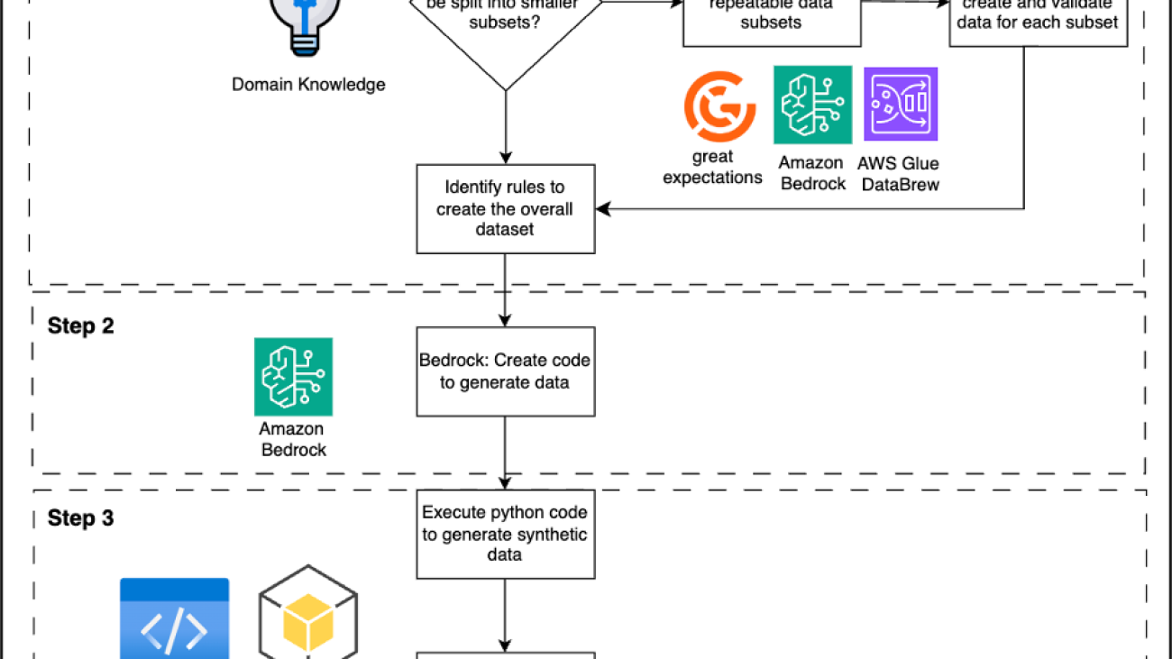
Build an enterprise synthetic data strategy using Amazon Bedrock
The AI landscape is rapidly evolving, and more organizations are recognizing the power of synthetic data to drive innovation. However, enterprises looking to use AI face a major roadblock: how to safely use sensitive data. Stringent privacy regulations make it risky to use such data, even with robust anonymization. Advanced analytics can potentially uncover hidden correlations and reveal real data, leading to compliance issues and reputational damage. Additionally, many industries struggle with a scarcity of high-quality, diverse datasets needed for critical processes like software testing, product development, and AI model training. This data shortage can hinder innovation, slowing down development cycles across various business operations.
Organizations need innovative solutions to unlock the potential of data-driven processes without compromising ethics or data privacy. This is where synthetic data comes in—a solution that mimics the statistical properties and patterns of real data while being entirely fictitious. By using synthetic data, enterprises can train AI models, conduct analyses, and develop applications without the risk of exposing sensitive information. Synthetic data effectively bridges the gap between data utility and privacy protection. However, creating high-quality synthetic data comes with significant challenges:
- Data quality – Making sure synthetic data accurately reflects real-world statistical properties and nuances is difficult. The data might not capture rare edge cases or the full spectrum of human interactions.
- Bias management – Although synthetic data can help reduce bias, it can also inadvertently amplify existing biases if not carefully managed. The quality of synthetic data heavily depends on the model and data used to generate it.
- Privacy vs. utility – Balancing privacy preservation with data utility is complex. There’s a risk of reverse engineering or data leakage if not properly implemented.
- Validation challenges – Verifying the quality and representation of synthetic data often requires comparison with real data, which can be problematic when working with sensitive information.
- Reality gap – Synthetic data might not fully capture the dynamic nature of the real world, potentially leading to a disconnect between model performance on synthetic data and real-world applications.
In this post, we explore how to use Amazon Bedrock for synthetic data generation, considering these challenges alongside the potential benefits to develop effective strategies for various applications across multiple industries, including AI and machine learning (ML). Amazon Bedrock offers a broad set of capabilities to build generative AI applications with a focus on security, privacy, and responsible AI. Built within the AWS landscape, Amazon Bedrock is designed to help maintain the security and compliance standards required for enterprise use.
Attributes of high-quality synthetic data
To be truly effective, synthetic data must be both realistic and reliable. This means it should accurately reflect the complexities and nuances of real-world data while maintaining complete anonymity. A high-quality synthetic dataset exhibits several key characteristics that facilitate its fidelity to the original data:
- Data structure – The synthetic data should maintain the same structure as the real data, including the same number of columns, data types, and relationships between different data sources
- Statistical properties – The synthetic data should mimic the statistical properties of the real data, such as mean, median, standard deviation, correlation between variables, and distribution patterns.
- Temporal patterns – If the real data exhibits temporal patterns (for example, diurnal or seasonal patterns), the synthetic data should also reflect these patterns.
- Anomalies and outliers – Real-world data often contains anomalies and outliers. The synthetic data should also include a similar proportion and distribution of anomalies and outliers to accurately represent the real-world scenario.
- Referential integrity – If the real data has relationships and dependencies between different data sources, the synthetic data should maintain these relationships to facilitate referential integrity.
- Consistency – The synthetic data should be consistent across different data sources and maintain the relationships and dependencies between them, facilitating a coherent and unified representation of the dataset.
- Scalability – The synthetic data generation process should be scalable to handle large volumes of data and support the generation of synthetic data for different scenarios and use cases.
- Diversity – The synthetic data should capture the diversity present in the real data.
Solution overview
Generating useful synthetic data that protects privacy requires a thoughtful approach. The following figure represents the high-level architecture of the proposed solution. The process involves three key steps:
- Identify validation rules that define the structure and statistical properties of the real data.
- Use those rules to generate code using Amazon Bedrock that creates synthetic data subsets.
- Combine multiple synthetic subsets into full datasets.

Let’s explore these three key steps for creating useful synthetic data in more detail.
Step 1: Define data rules and characteristics
- To create synthetic datasets, start by establishing clear rules that capture the essence of your target data:
- Use domain-specific knowledge to identify key attributes and relationships.
- Study existing public datasets, academic resources, and industry documentation.
- Use tools like AWS Glue DataBrew, Amazon Bedrock, or open source alternatives (such as Great Expectations) to analyze data structures and patterns.
- Develop a comprehensive rule-set covering:
- Data types and value ranges
- Inter-field relationships
- Quality standards
- Domain-specific patterns and anomalies
This foundational step makes sure your synthetic data accurately reflects real-world scenarios in your industry.
Step 2: Generate code with Amazon Bedrock
Transform your data rules into functional code using Amazon Bedrock language models:
- Choose an appropriate Amazon Bedrock model based on code generation capabilities and domain relevance.
- Craft a detailed prompt describing the desired code output, including data structures and generation rules.
- Use the Amazon Bedrock API to generate Python code based on your prompts.
- Iteratively refine the code by:
- Reviewing for accuracy and efficiency
- Adjusting prompts as needed
- Incorporating developer input for complex scenarios
The result is a tailored script that generates synthetic data entries matching your specific requirements and closely mimicking real-world data in your domain.
Step 3: Assemble and scale the synthetic dataset
Transform your generated data into a comprehensive, real-world representative dataset:
- Use the code from Step 2 to create multiple synthetic subsets for various scenarios.
- Merge subsets based on domain knowledge, maintaining realistic proportions and relationships.
- Align temporal or sequential components and introduce controlled randomness for natural variation.
- Scale the dataset to required sizes, reflecting different time periods or populations.
- Incorporate rare events and edge cases at appropriate frequencies.
- Generate accompanying metadata describing dataset characteristics and the generation process.
The end result is a diverse, realistic synthetic dataset for uses like system testing, ML model training, or data analysis. The metadata provides transparency into the generation process and data characteristics. Together, these measures result in a robust synthetic dataset that closely parallels real-world data while avoiding exposure of direct sensitive information. This generalized approach can be adapted to various types of datasets, from financial transactions to medical records, using the power of Amazon Bedrock for code generation and the expertise of domain knowledge for data validation and structuring.
Importance of differential privacy in synthetic data generation
Although synthetic data offers numerous benefits for analytics and machine learning, it’s essential to recognize that privacy concerns persist even with artificially generated datasets. As we strive to create high-fidelity synthetic data, we must also maintain robust privacy protections for the original data. Although synthetic data mimics patterns in actual data, if created improperly, it risks revealing details about sensitive information in the source dataset. This is where differential privacy enters the picture. Differential privacy is a mathematical framework that provides a way to quantify and control the privacy risks associated with data analysis. It works by injecting calibrated noise into the data generation process, making it virtually impossible to infer anything about a single data point or confidential information in the source dataset.
Differential privacy protects against re-identification exploits by adversaries attempting to extract details about data. The carefully calibrated noise added to synthetic data makes sure that even if an adversary tries, it is computationally infeasible to tie an output back to specific records in the original data, while still maintaining the overall statistical properties of the dataset. This allows the synthetic data to closely reflect real-world characteristics and remain useful for analytics and modeling while protecting privacy. By incorporating differential privacy techniques into the synthetic data generation process, you can create datasets that not only maintain statistical properties of the original data but also offer strong privacy guarantees. It enables organizations to share data more freely, collaborate on sensitive projects, and develop AI models with reduced risk of privacy breaches. For instance, in healthcare, differentially private synthetic patient data can accelerate research without compromising individual patient confidentiality.
As we continue to advance in the field of synthetic data generation, the incorporation of differential privacy is becoming not just a best practice, but a necessary component for responsible data science. This approach paves the way for a future where data utility and privacy protection coexist harmoniously, fostering innovation while safeguarding individual rights. However, although differential privacy offers strong theoretical guarantees, its practical implementation can be challenging. Organizations must carefully balance the trade-off between privacy and utility, because increasing privacy protection often comes at the cost of reduced data utility.
Build synthetic datasets for Trusted Advisor findings with Amazon Bedrock
In this post, we guide you through the process of creating synthetic datasets for AWS Trusted Advisor findings using Amazon Bedrock. Trusted Advisor provides real-time guidance to optimize your AWS environment, improving performance, security, and cost-efficiency through over 500 checks against AWS best practices. We demonstrate the synthetic data generation approach using the “Underutilized Amazon EBS Volumes” check (checkid: DAvU99Dc4C) as an example.
By following this post, you will gain practical knowledge on:
- Defining data rules for Trusted Advisor findings
- Using Amazon Bedrock to generate data creation code
- Assembling and scaling synthetic datasets
This approach can be applied across over 500 Trusted Advisor checks, enabling you to build comprehensive, privacy-aware datasets for testing, training, and analysis. Whether you’re looking to enhance your understanding of Trusted Advisor recommendations or develop new optimization strategies, synthetic data offers powerful possibilities.
Prerequisites
To implement this approach, you must have an AWS account with the appropriate permissions.
- AWS Account Setup:
- IAM permissions for:
- Amazon Bedrock
- AWS Trusted Advisor
- Amazon EBS
- IAM permissions for:
- AWS Service Access:
- Access enabled for Amazon Bedrock in your Region
- Access to Anthropic Claude model in Amazon Bedrock
- Enterprise or Business support plan for full Trusted Advisor access
- Development Environment:
- Python 3.8 or later installed
- Required Python packages:
- pandas
- numpy
- random
- boto3
- Knowledge Requirements:
- Basic understanding of:
- Python programming
- AWS services (especially EBS and Trusted Advisor)
- Data analysis concepts
- JSON/YAML file format
- Basic understanding of:
Define Trusted Advisor findings rules
Begin by examining real Trusted Advisor findings for the “Underutilized Amazon EBS Volumes” check. Analyze the structure and content of these findings to identify key data elements and their relationships. Pay attention to the following:
- Standard fields – Check ID, volume ID, volume type, snapshot ID, and snapshot age
- Volume attributes – Size, type, age, and cost
- Usage metrics – Read and write operations, throughput, and IOPS
- Temporal patterns – Volume type and size variations
- Metadata – Tags, creation date, and last attached date
As you study these elements, note the typical ranges, patterns, and distributions for each attribute. For example, observe how volume sizes correlate with volume types, or how usage patterns differ between development and production environments. This analysis will help you create a set of rules that accurately reflect real-world Trusted Advisor findings.
After analyzing real Trusted Advisor outputs for the “Underutilized Amazon EBS Volumes” check, we identified the following crucial patterns and rules:
- Volume type – Consider gp2, gp3, io1, io2, and st1 volume types. Verify the volume sizes are valid for volume types.
- Criteria – Represent multiple AWS Regions, with appropriate volume types. Correlate snapshot ages with volume ages.
- Data structure – Each finding should include the same columns.
The following is an example ruleset:
Generate code with Amazon Bedrock
With your rules defined, you can now use Amazon Bedrock to generate Python code for creating synthetic Trusted Advisor findings.
The following is an example prompt for Amazon Bedrock:
You can submit this prompt to the Amazon Bedrock chat playground using Anthropic’s Claude 3.5 Sonnet on Amazon Bedrock, and receive generated Python code. Review this code carefully, verifying it meets all specifications and generates realistic data. If necessary, iterate on your prompt or make manual adjustments to the code to address any missing logic or edge cases.
The resulting code will serve as the foundation for creating varied and realistic synthetic Trusted Advisor findings that adhere to the defined parameters. By using Amazon Bedrock in this way, you can quickly develop sophisticated data generation code that would otherwise require significant manual effort and domain expertise to create.
Create data subsets
With the code generated by Amazon Bedrock and refined with your custom functions, you can now create diverse subsets of synthetic Trusted Advisor findings for the “Underutilized Amazon EBS Volumes” check. This approach allows you to simulate a wide range of real-world scenarios. In the following sample code, we have customized the volume_id and snapshot_id format to begin with vol-9999 and snap-9999, respectively:
This code creates subsets that include:
- Various volume types and instance types
- Different levels of utilization
- Occasional misconfigurations (for example, underutilized volumes)
- Diverse regional distribution
Combine and scale the dataset
The process of combining and scaling synthetic data involves merging multiple generated datasets while introducing realistic anomalies to create a comprehensive and representative dataset. This step is crucial for making sure that your synthetic data reflects the complexity and variability found in real-world scenarios. Organizations typically introduce controlled anomalies at a specific rate (usually 5–10% of the dataset) to simulate various edge cases and unusual patterns that might occur in production environments. These anomalies help in testing system responses, developing monitoring solutions, and training ML models to identify potential issues.
When generating synthetic data for underutilized EBS volumes, you might introduce anomalies such as oversized volumes (5–10 times larger than needed), volumes with old snapshots (older than 365 days), or high-cost volumes with low utilization. For instance, a synthetic dataset might include a 1 TB gp2 volume that’s only using 100 GB of space, simulating a real-world scenario of overprovisioned resources. See the following code:
The following screenshot shows an example of sample rows generated.

Validate the synthetic Trusted Advisor findings
Data validation is a critical step that verifies the quality, reliability, and representativeness of your synthetic data. This process involves performing rigorous statistical analysis to verify that the generated data maintains proper distributions, relationships, and patterns that align with real-world scenarios. Validation should include both quantitative metrics (statistical measures) and qualitative assessments (pattern analysis). Organizations should implement comprehensive validation frameworks that include distribution analysis, correlation checks, pattern verification, and anomaly detection. Regular visualization of the data helps in identifying inconsistencies or unexpected patterns.
For EBS volume data, validation might include analyzing the distribution of volume sizes across different types (gp2, gp3, io1), verifying that cost correlations match expected patterns, and making sure that introduced anomalies (like underutilized volumes) maintain realistic proportions. For instance, validating that the percentage of underutilized volumes aligns with typical enterprise environments (perhaps 15–20% of total volumes) and that the cost-to-size relationships remain realistic across volume types.
The following figures show examples of our validation checks.
- The following screenshot shows statistics of the generated synthetic datasets.

- The following figure shows the proportion of underutilized volumes in the generated synthetic datasets.

- The following figure shows the distribution of volume sizes in the generated synthetic datasets.

- The following figure shows the distribution of volume types in the generated synthetic datasets.

- The following figure shows the distribution of snapshot ages in the generated synthetic datasets.

Enhancing synthetic data with differential privacy
After exploring the steps to create synthetic datasets for the Trusted Advisor “Underutilized Amazon EBS Volumes” check, it’s worth revisiting how differential privacy strengthens this approach. When a cloud consulting firm analyzes aggregated Trusted Advisor data across multiple clients, differential privacy through OpenDP provides the critical privacy-utility balance needed. By applying carefully calibrated noise to computations of underutilized volume statistics, consultants can generate synthetic datasets that preserve essential patterns across Regions and volume types while mathematically guaranteeing individual client confidentiality. This approach verifies that the synthetic data maintains sufficient accuracy for meaningful trend analysis and recommendations, while eliminating the risk of revealing sensitive client-specific infrastructure details or usage patterns—making it an ideal complement to our synthetic data generation pipeline.
Conclusion
In this post, we showed how to use Amazon Bedrock to create synthetic data for enterprise needs. By combining language models available in Amazon Bedrock with industry knowledge, you can build a flexible and secure way to generate test data. This approach helps create realistic datasets without using sensitive information, saving time and money. It also facilitates consistent testing across projects and avoids ethical issues of using real user data. Overall, this strategy offers a solid solution for data challenges, supporting better testing and development practices.
In part 2 of this series, we will demonstrate how to use pattern recognition for different datasets to automate rule-set generation needed for the Amazon Bedrock prompts to generate corresponding synthetic data.
About the authors
 Devi Nair is a Technical Account Manager at Amazon Web Services, providing strategic guidance to enterprise customers as they build, operate, and optimize their workloads on AWS. She focuses on aligning cloud solutions with business objectives to drive long-term success and innovation.
 Vishal Karlupia is a Senior Technical Account Manager/Lead at Amazon Web Services, Toronto. He specializes in generative AI applications and helps customers build and scale their AI/ML workloads on AWS. Outside of work, he enjoys being outdoors and keeping bonfires alive.
 Srinivas Ganapathi is a Principal Technical Account Manager at Amazon Web Services. He is based in Toronto, Canada, and works with games customers to run efficient workloads on AWS.
 Nicolas Simard is a Technical Account Manager based in Montreal. He helps organizations accelerate their AI adoption journey through technical expertise, architectural best practices, and enables them to maximize business value from AWS’s Generative AI capabilities.

Llama 4 family of models from Meta are now available in SageMaker JumpStart
Today, we’re excited to announce the availability of Llama 4 Scout and Maverick models in Amazon SageMaker JumpStart and coming soon in Amazon Bedrock. Llama 4 represents Meta’s most advanced multimodal models to date, featuring a mixture of experts (MoE) architecture and context window support up to 10 million tokens. With native multimodality and early fusion technology, Meta states that these new models demonstrate unprecedented performance across text and vision tasks while maintaining efficient compute requirements. With a dramatic increase on supported context length from 128K in Llama 3, Llama 4 is now suitable for multi-document summarization, parsing extensive user activity for personalized tasks, and reasoning over extensive codebases. You can now deploy the Llama-4-Scout-17B-16E-Instruct, Llama-4-Maverick-17B-128E-Instruct, and Llama-4-Maverick-17B-128E-Instruct-FP8 models using SageMaker JumpStart in the US East (N. Virginia) AWS Region.
In this blog post, we walk you through how to deploy and prompt a Llama-4-Scout-17B-16E-Instruct model using SageMaker JumpStart.
Llama 4 overview
Meta announced Llama 4 today, introducing three distinct model variants: Scout, which offers advanced multimodal capabilities and a 10M token context window; Maverick, a cost-effective solution with a 128K context window; and Behemoth, in preview. These models are optimized for multimodal reasoning, multilingual tasks, coding, tool-calling, and powering agentic systems.
Llama 4 Maverick is a powerful general-purpose model with 17 billion active parameters, 128 experts, and 400 billion total parameters, and optimized for high-quality general assistant and chat use cases. Additionally, Llama 4 Maverick is available with base and instruct models in both a quantized version (FP8) for efficient deployment on the Instruct model and a non-quantized (BF16) version for maximum accuracy.
Llama 4 Scout, the more compact and smaller model, has 17 billion active parameters, 16 experts, and 109 billion total parameters, and features an industry-leading 10M token context window. These models are designed for industry-leading performance in image and text understanding with support for 12 languages, enabling the creation of AI applications that bridge language barriers.
See Meta’s community license agreement for usage terms and more details.
SageMaker JumpStart overview
SageMaker JumpStart offers access to a broad selection of publicly available foundation models (FMs). These pre-trained models serve as powerful starting points that can be deeply customized to address specific use cases. You can use state-of-the-art model architectures—such as language models, computer vision models, and more—without having to build them from scratch.
With SageMaker JumpStart, you can deploy models in a secure environment. The models can be provisioned on dedicated SageMaker inference instances can be isolated within your virtual private cloud (VPC). After deploying an FM, you can further customize and fine-tune it using the extensive capabilities of Amazon SageMaker AI, including SageMaker inference for deploying models and container logs for improved observability. With SageMaker AI, you can streamline the entire model deployment process.
Prerequisites
To try the Llama 4 models in SageMaker JumpStart, you need the following prerequisites:
- An AWS account that will contain all your AWS resources.
- An AWS Identity and Access Management (IAM) role to access SageMaker AI. To learn more about how IAM works with SageMaker AI, see Identity and Access Management for Amazon SageMaker AI.
- Access to Amazon SageMaker Studio and a SageMaker AI notebook instance or an interactive development environment (IDE) such as PyCharm or Visual Studio Code. We recommend using SageMaker Studio for straightforward deployment and inference.
- Access to accelerated instances (GPUs) for hosting the LLMs.
Discover Llama 4 models in SageMaker JumpStart
SageMaker JumpStart provides FMs through two primary interfaces: SageMaker Studio and the Amazon SageMaker Python SDK. This provides multiple options to discover and use hundreds of models for your specific use case.
SageMaker Studio is a comprehensive integrated development environment (IDE) that offers a unified, web-based interface for performing all aspects of the AI development lifecycle. From preparing data to building, training, and deploying models, SageMaker Studio provides purpose-built tools to streamline the entire process.
In SageMaker Studio, you can access SageMaker JumpStart to discover and explore the extensive catalog of FMs available for deployment to inference capabilities on SageMaker Inference. You can access SageMaker JumpStart by choosing JumpStart in the navigation pane or by choosing JumpStart from the Home page in SageMaker Studio, as shown in the following figure.

Alternatively, you can use the SageMaker Python SDK to programmatically access and use SageMaker JumpStart models. This approach allows for greater flexibility and integration with existing AI and machine learning (AI/ML) workflows and pipelines.
By providing multiple access points, SageMaker JumpStart helps you seamlessly incorporate pre-trained models into your AI/ML development efforts, regardless of your preferred interface or workflow.
Deploy Llama 4 models for inference through the SageMaker JumpStart UI
On the SageMaker JumpStart landing page, you can find all the public pre-trained models offered by SageMaker AI. You can then choose the Meta model provider tab to discover all the available Meta models.
If you’re using SageMaker Classic Studio and don’t see the Llama 4 models, update your SageMaker Studio version by shutting down and restarting. For more information about version updates, see Shut down and Update Studio Classic Apps.
- Search for Meta to view the Meta model card. Each model card shows key information, including:
- Model name
- Provider name
- Task category (for example, Text Generation)
- Select the model card to view the model details page.

The model details page includes the following information:
- The model name and provider information
- Deploy button to deploy the model
- About and Notebooks tabs with detailed information
The About tab includes important details, such as:
- Model description
- License information
- Technical specifications
- Usage guidelines
Before you deploy the model, we recommended you review the model details and license terms to confirm compatibility with your use case.
- Choose Deploy to proceed with deployment.
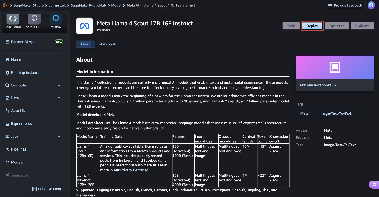
- For Endpoint name, use the automatically generated name or enter a custom one.
- For Instance type, use the default: p5.48xlarge.
- For Initial instance count, enter the number of instances (default: 1).
Selecting appropriate instance types and counts is crucial for cost and performance optimization. Monitor your deployment to adjust these settings as needed. - Under Inference type, Real-time inference is selected by default. This is optimized for sustained traffic and low latency.
- Review all configurations for accuracy. For this model, we strongly recommend adhering to SageMaker JumpStart default settings and making sure that network isolation remains in place.
- Choose Deploy. The deployment process can take several minutes to complete.

When deployment is complete, your endpoint status will change to InService. At this point, the model is ready to accept inference requests through the endpoint. You can monitor the deployment progress on the SageMaker console Endpoints page, which will display relevant metrics and status information. When the deployment is complete, you can invoke the model using a SageMaker runtime client and integrate it with your applications.
Deploy Llama 4 models for inference using the SageMaker Python SDK
When you choose Deploy and accept the terms, model deployment will start. Alternatively, you can deploy through the example notebook by choosing Open Notebook. The notebook provides end-to-end guidance on how to deploy the model for inference and clean up resources.
To deploy using a notebook, start by selecting an appropriate model, specified by the model_id. You can deploy any of the selected models on SageMaker AI.
You can deploy the Llama 4 Scout model using SageMaker JumpStart with the following SageMaker Python SDK code:
This deploys the model on SageMaker AI with default configurations, including default instance type and default VPC configurations. You can change these configurations by specifying non-default values in JumpStartModel. To successfully deploy the model, you must manually set accept_eula=True as a deploy method argument. After it’s deployed, you can run inference against the deployed endpoint through the SageMaker predictor:
Recommended instances and benchmark
The following table lists all the Llama 4 models available in SageMaker JumpStart along with the model_id, default instance types, and the maximum number of total tokens (sum of number of input tokens and number of generated tokens) supported for each of these models. For increased context length, you can modify the default instance type in the SageMaker JumpStart UI.
| Model name | Model ID | Default instance type | Supported instance types |
| Llama-4-Scout-17B-16E-Instruct | meta-vlm-llama-4-scout-17b-16e-instruct |
ml.p5.48xlarge | ml.g6e.48xlarge, ml.p5.48xlarge, ml.p5en.48xlarge |
| Llama-4-Maverick-17B-128E-Instruct | meta-vlm-llama-4-maverick-17b-128e-instruct |
ml.p5.48xlarge | ml.p5.48xlarge, ml.p5en.48xlarge |
| Llama 4-Maverick-17B-128E-Instruct-FP8 | meta-vlm-llama-4-maverick-17b-128-instruct-fp8 |
ml.p5.48xlarge | ml.p5.48xlarge, ml.p5en.48xlarge |
Inference and example prompts for Llama 4 Scout 17B 16 Experts model
You can use the Llama 4 Scout model for text and image or vision reasoning use cases. With that model, you can perform a variety of tasks, such as image captioning, image text retrieval, visual question answering and reasoning, document visual question answering, and more.
In the following sections we show example payloads, invocations, and responses for Llama 4 Scout that you can use against your Llama 4 model deployments using Sagemaker JumpStart.
Text-only input
Input:
Response:
Single-image input
In this section, let’s test Llama 4’s multimodal capabilities. By merging text and vision tokens into a unified processing backbone, Llama 4 can seamlessly understand and respond to queries about an image. The following is an example of how you can prompt Llama 4 to answer questions about an image such as the one in the example:
Image:

Input:
Response:
The Llama 4 model on JumpStart can take in the image provided via a URL, underlining its powerful potential for real-time multimodal applications.
Multi-image input
Building on its advanced multimodal functionality, Llama 4 can effortlessly process multiple images at the same time. In this demonstration, the model is prompted with two image URLs and tasked with describing each image and explaining their relationship, showcasing its capacity to synthesize information across several visual inputs. Let’s test this below by passing in the URLs of the following images in the payload.
Image 1:

Image 2:

Input:
Response:
As you can see, Llama 4 excels in handling multiple images simultaneously, providing detailed and contextually relevant insights that emphasize its robust multimodal processing abilities.
Codebase analysis with Llama 4
Using Llama 4 Scout’s industry-leading context window, this section showcases its ability to deeply analyze expansive codebases. The example extracts and contextualizes the buildspec-1-10-2.yml file from the AWS Deep Learning Containers GitHub repository, illustrating how the model synthesizes information across an entire repository. We used a tool to ingest the whole repository into plaintext that we provided to the model as context:
Input:
Output:
Multi-document processing
Harnessing the same extensive token context window, Llama 4 Scout excels in multi-document processing. In this example, the model extracts key financial metrics from Amazon 10-K reports (2017-2024), demonstrating its capability to integrate and analyze data spanning multiple years—all without the need for additional processing tools.
Input:
Output:
Clean up
To avoid incurring unnecessary costs, when you’re done, delete the SageMaker endpoints using the following code snippets:
Alternatively, using the SageMaker console, complete the following steps:
- On the SageMaker console, under Inference in the navigation pane, choose Endpoints.
- Search for the embedding and text generation endpoints.
- On the endpoint details page, choose Delete.
- Choose Delete again to confirm.
Conclusion
In this post, we explored how SageMaker JumpStart empowers data scientists and ML engineers to discover, access, and deploy a wide range of pre-trained FMs for inference, including Meta’s most advanced and capable models to date. Get started with SageMaker JumpStart and Llama 4 models today.
For more information about SageMaker JumpStart, see Train, deploy, and evaluate pretrained models with SageMaker JumpStart and Getting started with Amazon SageMaker JumpStart.
About the authors
 Marco Punio is a Sr. Specialist Solutions Architect focused on generative AI strategy, applied AI solutions, and conducting research to help customers hyper-scale on AWS. As a member of the Third-party Model Provider Applied Sciences Solutions Architecture team at AWS, he is a global lead for the Meta–AWS Partnership and technical strategy. Based in Seattle, Washington, Marco enjoys writing, reading, exercising, and building applications in his free time.
 Chakravarthy Nagarajan is a Principal Solutions Architect specializing in machine learning, big data, and high performance computing. In his current role, he helps customers solve real-world, complex business problems using machine learning and generative AI solutions.
 Banu Nagasundaram leads product, engineering, and strategic partnerships for Amazon SageMaker JumpStart, the SageMaker machine learning and generative AI hub. She is passionate about building solutions that help customers accelerate their AI journey and unlock business value.
 Malav Shastri is a Software Development Engineer at AWS, where he works on the Amazon SageMaker JumpStart and Amazon Bedrock teams. His role focuses on enabling customers to take advantage of state-of-the-art open source and proprietary foundation models and traditional machine learning algorithms. Malav holds a Master’s degree in Computer Science.
 Niithiyn Vijeaswaran is a Generative AI Specialist Solutions Architect with the Third-party Model Science team at AWS. His area of focus is AWS AI accelerators (AWS Neuron). He holds a Bachelor’s degree in Computer Science and Bioinformatics.
 Baladithya Balamurugan is a Solutions Architect at AWS focused on ML deployments for inference and using AWS Neuron to accelerate training and inference. He works with customers to enable and accelerate their ML deployments on services such as Amazon Sagemaker and Amazon EC2. Based in San Francisco, Baladithya enjoys tinkering, developing applications, and his home lab in his free time.
 John Liu has 14 years of experience as a product executive and 10 years of experience as a portfolio manager. At AWS, John is a Principal Product Manager for Amazon Bedrock. Previously, he was the Head of Product for AWS Web3 and Blockchain. Prior to AWS, John held various product leadership roles at public blockchain protocols and fintech companies, and also spent 9 years as a portfolio manager at various hedge funds.
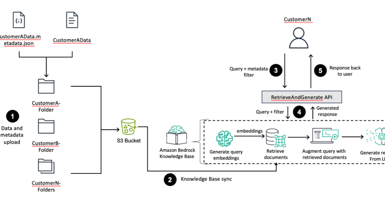
Multi-tenancy in RAG applications in a single Amazon Bedrock knowledge base with metadata filtering
Amazon Bedrock is a fully managed service that offers a choice of high-performing foundation models (FMs) from leading AI companies and AWS. Amazon Bedrock Knowledge Bases offers fully managed, end-to-end Retrieval Augmented Generation (RAG) workflows to create highly accurate, low-latency, secure, and custom generative AI applications by incorporating contextual information from your company’s data sources.
Organizations need to control access to their data across different business units, including companies, departments, or even individuals, while maintaining scalability. When organizations try to separate data sources manually, they often create unnecessary complexity and hit service limitations. This post demonstrates how Amazon Bedrock Knowledge Bases can help you scale your data management effectively while maintaining proper access controls on different management levels.
One of these strategies is using Amazon Simple Storage Service (Amazon S3) folder structures and Amazon Bedrock Knowledge Bases metadata filtering to enable efficient data segmentation within a single knowledge base. Additionally, we dive into integrating common vector database solutions available for Amazon Bedrock Knowledge Bases and how these integrations enable advanced metadata filtering and querying capabilities.
Organizing S3 folder structures for scalable knowledge bases
Organizations working with multiple customers need a secure and scalable way to keep each customer’s data separate while maintaining efficient access controls. Without proper data segregation, companies risk exposing sensitive information between customers or creating complex, hard-to-maintain systems. For this post, we focus on maintaining access controls across multiple business units within the same management level.
A key strategy involves using S3 folder structures and Amazon Bedrock Knowledge Bases metadata filtering to enable efficient data segregation within a single knowledge base. Instead of creating separate knowledge bases for each customer, you can use a consolidated knowledge base with a well-structured S3 folder hierarchy. For example, imagine a consulting firm that manages documentation for multiple healthcare providers—each customer’s sensitive patient records and operational documents must remain strictly separated. The Amazon S3 structure might look as follows:
s3://amzn-s3-demo-my-knowledge-base-bucket/customer-data/
s3://amzn-s3-demo-my-knowledge-base-bucket/customer-data/customerA/
s3://amzn-s3-demo-my-knowledge-base-bucket/customer-data/customerA/policies/
s3://amzn-s3-demo-my-knowledge-base-bucket/customer-data/customerA/procedures/
s3://amzn-s3-demo-my-knowledge-base-bucket/customer-data/customerB/
s3://amzn-s3-demo-my-knowledge-base-bucket/customer-data/customerB/policies/
s3://amzn-s3-demo-my-knowledge-base-bucket/customer-data/customerB/procedures/
This structure makes sure that Customer A’s healthcare documentation remains completely separate from Customer B’s data. When combined with Amazon Bedrock Knowledge Bases metadata filtering, you can verify that users associated with Customer A can only access their organization’s documents, and Customer B’s users can only see their own data—maintaining strict data boundaries while using a single, efficient knowledge base infrastructure.
The Amazon Bedrock Knowledge Bases metadata filtering capability enhances this segregation by allowing you to tag documents with customer-specific identifiers and other relevant attributes. These metadata filters provide an additional layer of security and organization, making sure that queries only return results from the appropriate customer’s dataset.
Solution overview
The following diagram provides a high-level overview of AWS services and features through a sample use case. Although the example uses Customer A and Customer B for illustration, these can represent distinct business units (such as departments, companies, or teams) with different compliance requirements, rather than only individual customers.

The workflow consists of the following steps:
- Customer data is uploaded along with metadata indicating data ownership and other properties to specific folders in an S3 bucket.
- The S3 bucket, containing customer data and metadata, is configured as a knowledge base data source. Amazon Bedrock Knowledge Bases ingests the data, along with the metadata, from the source repository and a knowledge base sync is performed.
- A customer initiates a query using a frontend application with metadata filters against the Amazon Bedrock knowledge base. An access control metadata filter must be in place to make sure that the customer only accesses data they own; the customer can apply additional filters to further refine query results. This combined query and filter is passed to the
RetrieveAndGenerateAPI. - The
RetrieveAndGenerateAPI handles the core RAG workflow. It consists of several sub-steps:- The user query is converted into a vector representation (embedding).
- Using the query embedding and the metadata filter, relevant documents are retrieved from the knowledge base.
- The original query is augmented with the retrieved documents, providing context for the large language model (LLM).
- The LLM generates a response based on the augmented query and retrieved context.
- Finally, the generated response is sent back to the user.
When implementing Amazon Bedrock Knowledge Bases in scenarios involving sensitive information or requiring access controls, developers must implement proper metadata filtering in their application code. Failure to enforce appropriate metadata-based filtering could result in unauthorized access to sensitive documents within the knowledge base. Metadata filtering serves as a critical security boundary and should be consistently applied across all queries. For comprehensive guidance on implementing secure metadata filtering practices, refer to the Amazon Bedrock Knowledge Base Security documentation.
Implement metadata filtering
For this use case, two specific example customers, Customer A and Customer B, are aligned to different proprietary compliance documents. The number of customers and folders can scale to N depending on the size of the customer base. We will use the following public documents, which will reside in the respective customer’s S3 folder. Customer A requires the Architecting for HIPAA Security and Compliance on AWS document. Customer B requires access to the Using AWS in the Context of NHS Cloud Security Guidance document.
- Create a JSON file representing the corresponding metadata for both Customer A and Customer B:
The following is the JSON metadata for Customer A’s data:
{ "metadataAttributes": { "customer": "CustomerA", "documentType": "HIPAA Compliance Guide", "focus": "HIPAA Compliance", "publicationYear": 2022, "region": "North America" }}
The following is the JSON metadata for Customer B’s data:
{ "metadataAttributes": { "customer": "CustomerB", "documentType": "NHS Compliance Guidance", "focus": "UK Healthcare Compliance", "publicationYear": 2023, "region": "Europe" }}
- Save these files separately with the naming convention <filename>.pdf.metadata.JSON and store them in the same S3 folder or prefix that stores the source document. For Customer A, name the metadata file architecting-hipaa-compliance-on-aws.pdf.metadata.json and upload it to the folder corresponding to Customer A’s documents. Repeat these steps for Customer B.

- Create an Amazon Bedrock knowledge base. For instructions, see Create a knowledge base by connecting to a data source in Amazon Bedrock Knowledge Bases
- After you create your knowledge base, you can sync the data source. For more details, see Sync your data with your Amazon Bedrock knowledge base.
Test metadata filtering
After you sync the data source, you can test the metadata filtering.
The following is an example for setting the customer = CustomerA metadata filter to show Customer A only has access to the HIPAA compliance document and not the NHS Compliance Guidance that relates to Customer B.
To use the metadata filtering options on the Amazon Bedrock console, complete the following steps:
- On the Amazon Bedrock console, choose Knowledge Bases in the navigation pane.
- Choose the knowledge base you created.
- Choose Test knowledge base.
- Choose the Configurations icon, then expand Filters.
- Enter a condition using the format: key = value (for this example,
customer = CustomerA) and press Enter. - When finished, enter your query in the message box, then choose Run.
We enter two queries, “summarize NHS Compliance Guidance” and “summarize HIPAA Compliance Guide.” The following figure shows the two queries: one attempting to query data related to NHS compliance guidance, which fails because it is outside of the Customer A segment, and another successfully querying data on HIPAA compliance, which has been tagged for Customer A.

Implement field-specific chunking
Amazon Bedrock Knowledge Bases supports several document types for Amazon S3 metadata filtering. The supported file formats include:
- Plain text (.txt)
- Markdown (.md)
- HTML (.html)
- Microsoft Word documents (.doc and.docx)
- CSV files (.csv)
- Microsoft Excel spreadsheets (.xls and .xlsx)
When working with CSV data, customers often want to chunk on a specific field in their CSV documents to gain granular control over data retrieval and enhance the efficiency and accuracy of queries. By creating logical divisions based on fields, users can quickly access relevant subsets of data without needing to process the entire dataset.
Additionally, field-specific chunking aids in organizing and maintaining large datasets, facilitating updating or modifying specific portions without affecting the whole. This granularity supports better version control and data lineage tracking, which are crucial for data integrity and compliance. Focusing on relevant chunks can improve the performance of LLMs, ultimately leading to more accurate insights and better decision-making processes within organizations. For more information, see Amazon Bedrock Knowledge Bases now supports advanced parsing, chunking, and query reformulation giving greater control of accuracy in RAG based applications.
To demonstrate field-specific chunking, we use two sample datasets with the following schemas:
- Schema 1 – Customer A uses the following synthetic dataset for recording medical case reports (
case_reports.csv)
| CaseID | DoctorID | PatientID | Diagnosis | TreatmentPlan | Content |
| C001 | D001 | P001 | Hypertension | Lifestyle changes, Medication (Lisinopril) | “Patient diagnosed with hypertension, advised lifestyle changes, and started on Lisinopril.” |
| C002 | D002 | P002 | Diabetes Type 2 | Medication (Metformin), Diet adjustment | “Diabetes Type 2 confirmed, prescribed Metformin, and discussed a low-carb diet plan.” |
| C003 | D003 | P003 | Asthma | Inhaler (Albuterol) | “Patient reports difficulty breathing; prescribed Albuterol inhaler for asthma management.” |
| C004 | D004 | P004 | Coronary Artery Disease | Medication (Atorvastatin), Surgery Consultation | “Coronary artery disease diagnosed, started on Atorvastatin, surgery consultation recommended.” |
| … | … | … | … | … | … |
- Schema 2 – Customer B uses the following dataset for recording genetic testing results (
genetic_testings.csv)
| SampleID | PatientID | TestType | Result |
| S001 | P001 | Genome Sequencing | Positive |
| S002 | P002 | Exome Sequencing | Negative |
| S003 | P003 | Targeted Gene Panel | Positive |
| S004 | P004 | Whole Genome Sequencing | Negative |
| … | … | … | … |
Complete the following steps:
- Create a JSON file representing the corresponding metadata for both Customer A and Customer B:
The following is the JSON metadata for Customer A’s data (note that recordBasedStructureMetadata supports exactly one content field):
The following is the JSON metadata for Customer B’s data:
- Save your files with the naming convention <filename>.csv.metadata.json and store the new JSON file in the same S3 prefix of the bucket where you stored the dataset. For Customer A, name the metadata file case_reports.csv.metadata.JSON and upload the file to the same folder corresponding to Customer A’s datasets.

Repeat the process for Customer B. You have now created metadata from the source CSV itself, as well as an additional metadata field customer that doesn’t exist in the original dataset. The following image highlights the metadata.
Test field-specific chunking
The following is an example of setting the customer = CustomerA metadata filter demonstrating that Customer A only has access to the medical case reports dataset and not the genetic testing dataset that relates to Customer B. We enter a query requesting information about a patient with PatientID as P003.
To test, complete the following steps:
- On the Amazon Bedrock console, choose Knowledge Bases in the navigation pane.
- Choose the knowledge base you created.
- Choose Test knowledge base.
- Choose the Configurations icon, then expand Filters.
- Enter a condition using the format: key = value (for this example,
customer = CustomerA) and press Enter. - When finished, enter your query in the message box, then choose Run.
The knowledge base returns, “Patient reports difficulty breathing; prescribed Albuterol inhaler for asthma management,” which is the Result column entry from Customer A’s medical case reports dataset for that PatientID. Although there is a record with the same PatientID in Customer B’s genetic testing dataset, Customer A has access only to the medical case reports data due to the metadata filtering.
Apply metadata filtering for the Amazon Bedrock API
You can call the Amazon Bedrock API RetrieveAndGenerate to query a knowledge base and generate responses based on the retrieved results using the specified FM or inference profile. The response only cites sources that are relevant to the query.
The following Python Boto3 example API call applies the metadata filtering for retrieving Customer B data and generates responses based on the retrieved results using the specified FM (Anthropic’s Claude 3 Sonnet) in RetrieveAndGenerate:
The following GitHub repository provides a notebook that you can follow to deploy an Amazon Bedrock knowledge base with access control implemented using metadata filtering in your own AWS account.
Integrate existing vector databases with Amazon Bedrock Knowledge Bases and validate metadata
There are multiple ways to create vector databases from AWS services and partner offerings to build scalable solutions. If a vector database doesn’t exist, you can use Amazon Bedrock Knowledge Bases to create one using Amazon OpenSearch Serverless Service, Amazon Aurora PostgreSQL Serverless, or Amazon Neptune Analytics to store embeddings, or you can specify an existing vector database supported by Redis Enterprise Cloud, Amazon Aurora PostgreSQL with the pgvector extension, MongoDB Atlas, or Pinecone. After you create your knowledge base and either ingest or sync your data, the metadata attached to the data will be ingested and automatically populated to the vector database.
In this section, we review how to incorporate and validate metadata filtering with existing vector databases using OpenSearch Serverless, Aurora PostgreSQL with the pgvector extension, and Pinecone. To learn how to set up each individual vector databases, follow the instructions in Prerequisites for your own vector store for a knowledge base.
OpenSearch Serverless as a knowledge base vector store
With OpenSearch Serverless vector database capabilities, you can implement semantic search, RAG with LLMs, and recommendation engines. To address data segregation between business segments within each Amazon Bedrock knowledge base with an OpenSearch Serverless vector database, use metadata filtering. Metadata filtering allows you to segment data inside of an OpenSearch Serverless vector database. This can be useful when you want to add descriptive data to your documents for more control and granularity in searches.
Each OpenSearch Serverless dashboard has a URL that can be used to add documents and query your database; the structure of the URL is domain-endpoint/_dashboard.
After creating a vector database index, you can use metadata filtering to selectively retrieve items by using JSON query options in the request body. For example, to return records owned by Customer A, you can use the following request:
This query will return a JSON response containing the document index with the document labeled as belonging to Customer A.
Aurora PostgreSQL with the pgvector extension as a knowledge base vector store
Pgvector is an extension of PostgreSQL that allows you to extend your relational database into a high-dimensional vector database. It stores each document’s vector in a separate row of a database table. For details on creating an Aurora PostgreSQL table to be used as the vector store for a knowledge base, see Using Aurora PostgreSQL as a Knowledge Base for Amazon Bedrock.
When storing a vector index for your knowledge base in an Aurora database cluster, make sure that the table for your index contains a column for each metadata property in your metadata files before starting data ingestion.
Continuing with the Customer A example, the customer requires the Architecting for HIPAA Security and Compliance on AWS document.
The following is the JSON metadata for Customer A’s data:
{ "metadataAttributes": { "customer": "CustomerA", "documentType": "HIPAA Compliance Guide", "focus": "HIPAA Compliance", "publicationYear": 2022, "region": "North America" }}
The schema of the PostgreSQL table you create must contain four essential columns for ID, text content, vector values, and service managed metadata; it must also include additional metadata columns (customer, documentType, focus, publicationYear, region) for each metadata property in the corresponding metadata file. This allows pgvector to perform efficient vector searches and similarity comparisons by running queries directly on the database table. The following table summarizes the columns.
| Column Name | Data Type | Description |
| id | UUID primary key | Contains unique identifiers for each record |
| chunks | Text | Contains the chunks of raw text from your data sources |
| embedding | Vector | Contains the vector embeddings of the data sources |
| metadata | JSON | Contains Amazon Bedrock managed metadata required to carry out source attribution and to enable data ingestion and querying. |
| customer | Text | Contains the customer ID |
| documentType | Text | Contains the type of document |
| focus | Text | Contains the document focus |
| publicationYear | Int | Contains the year document was published |
| region | Text | Contains the document’s related AWS Region |
During Amazon Bedrock knowledge base data ingestion, these columns will be populated with the corresponding attribute values. Chunking can break down a single document into multiple separate records (each associated with a different ID).
This PostgreSQL table structure allows for efficient storage and retrieval of document vectors, using PostgreSQL’s robustness and pgvector’s specialized vector handling capabilities for applications like recommendation systems, search engines, or other systems requiring similarity searches in high-dimensional space.
Using this approach, you can implement access control at the table level by creating database tables for each segment. Additional metadata columns can also be included in the table for properties such as the specific document owner (user_id), tags, and so on to further enable and enforce fine-grained (row-level) access control and result filtering if you restrict each user to only query the rows that contain their user ID (document owner).
After creating a vector database table, you can use metadata filtering to selectively retrieve items by using a PostgreSQL query. For example, to return table records owned by Customer A, you can use the following query:
This query will return a response containing the database records with the document labeled as belonging to Customer A.
Pinecone as a knowledge base vector store
Pinecone, a fully managed vector database, enables semantic search, high-performance search, and similarity matching. Pinecone databases can be integrated into your AWS environment in the form of Amazon Bedrock knowledge bases, but are first created through the Pinecone console. For detailed documentation about setting up a vector store in Pinecone, see Pinecone as a Knowledge Base for Amazon Bedrock. Then, you can integrate the databases using the Amazon Bedrock console. For more information about Pinecone integration with Amazon Bedrock, see Bring reliable GenAI applications to market with Amazon Bedrock and Pinecone.
You can segment a Pinecone database by adding descriptive metadata to each index and using that metadata to inform query results. Pinecone supports strings and lists of strings to filter vector searches on customer names, customer industry, and so on. Pinecone also supports numbers and booleans.
Use metadata query language to filter output ($eq, $ne, $in, $nin, $and, and $or). The following example shows a snippet of metadata and queries that will return that index. The example queries in Python demonstrate how you can retrieve a list of records associated with Customer A from the Pinecone database.
This query will return a response containing the database records labeled as belonging to Customer A.
Enhanced scaling with multiple data sources
Amazon Bedrock Knowledge Bases now supports multiple data sources across AWS accounts. Amazon Bedrock Knowledge Bases can ingest data from up to five data sources, enhancing the comprehensiveness and relevancy of a knowledge base. This feature allows customers with complex IT systems to incorporate data into generative AI applications without restructuring or migrating data sources. It also provides flexibility for you to scale your Amazon Bedrock knowledge bases when data resides in different AWS accounts.
The features includes cross-account data access, enabling the configuration of S3 buckets as data sources across different accounts and efficient data management options for retaining or deleting data when a source is removed. These enhancements alleviate the need for creating multiple knowledge bases or redundant data copies.
Clean up
After completing the steps in this blog post, make sure to clean up your resources to avoid incurring unnecessary charges. Delete the Amazon Bedrock Knowledge Base by navigating to the Amazon Bedrock console, selecting your knowledge base, and choosing “Delete” from the “Actions” dropdown menu. If you created vector databases for testing, remember to delete OpenSearch Serverless collections, stop or delete Aurora PostgreSQL instances, and remove Pinecone index created. Additionally, consider deleting test documents uploaded to S3 buckets specifically for this blog example to avoid storage charges. Review and clean up any IAM roles or policies created for this demonstration if they’re no longer needed.
While Amazon Bedrock Knowledge Bases include charges for data indexing and queries, the underlying storage in S3 and vector databases will continue to incur charges until those resources are removed. For specific pricing details, refer to the Amazon Bedrock pricing page.
Conclusion
In this post, we covered several key strategies for building scalable, secure, and segmented Amazon Bedrock knowledge bases. These include using S3 folder structure, metadata to organize data sources, and data segmentation within a single knowledge base. Using metadata filtering to create custom queries that target specific data segments helps provide retrieval accuracy and maintain data privacy. We also explored integrating and validating metadata for vector databases including OpenSearch Serverless, Aurora PostgreSQL with the pgvector extension, and Pinecone.
By consolidating multiple business segments or customer data within a single Amazon Bedrock knowledge base, organizations can achieve cost optimization compared to creating and managing them separately. The improved data segmentation and access control measures help make sure each team or customer can only access the information relevant to their domain. The enhanced scalability helps meet the diverse needs of organizations, while maintaining the necessary data segregation and access control.
Try out metadata filtering with Amazon Bedrock Knowledge Bases, and share your thoughts and questions with the authors or in the comments.
About the Authors
 Breanne Warner is an Enterprise Solutions Architect at Amazon Web Services supporting healthcare and life science customers. She is passionate about supporting customers to use generative AI on AWS and evangelizing 1P and 3P model adoption. Breanne is also on the Women at Amazon board as co-director of Allyship with the goal of fostering inclusive and diverse culture at Amazon. Breanne holds a Bachelor of Science in Computer Engineering from University of Illinois at Urbana Champaign.
 Justin Lin is a Small & Medium Business Solutions Architect at Amazon Web Services. He studied computer science at UW Seattle. Dedicated to designing and developing innovative solutions that empower customers, Justin has been dedicating his time to experimenting with applications in generative AI, natural language processing, and forecasting.
 Chloe Gorgen is an Enterprise Solutions Architect at Amazon Web Services, advising AWS customers in various topics including security, analytics, data management, and automation. Chloe is passionate about youth engagement in technology, and supports several AWS initiatives to foster youth interest in cloud-based technology. Chloe holds a Bachelor of Science in Statistics and Analytics from the University of North Carolina at Chapel Hill.
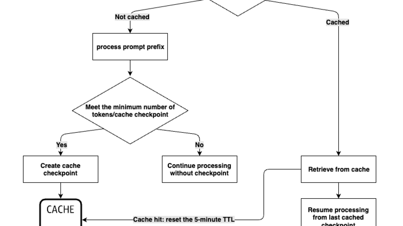
Effectively use prompt caching on Amazon Bedrock
Prompt caching, now generally available on Amazon Bedrock with Anthropic’s Claude 3.5 Haiku and Claude 3.7 Sonnet, along with Nova Micro, Nova Lite, and Nova Pro models, lowers response latency by up to 85% and reduces costs up to 90% by caching frequently used prompts across multiple API calls.
With prompt caching, you can mark the specific contiguous portions of your prompts to be cached (known as a prompt prefix). When a request is made with the specified prompt prefix, the model processes the input and caches the internal state associated with the prefix. On subsequent requests with a matching prompt prefix, the model reads from the cache and skips the computation steps required to process the input tokens. This reduces the time to first token (TTFT) and makes more efficient use of hardware such that we can share the cost savings with you.
This post provides a detailed overview of the prompt caching feature on Amazon Bedrock and offers guidance on how to effectively use this feature to achieve improved latency and cost savings.
How prompt caching works
Large language model (LLM) processing is made up of two primary stages: input token processing and output token generation. The prompt caching feature on Amazon Bedrock optimizes the input token processing stage.
You can begin by marking the relevant portions of your prompt with cache checkpoints. The entire section of the prompt preceding the checkpoint then becomes the cached prompt prefix. As you send more requests with the same prompt prefix, marked by the cache checkpoint, the LLM will check if the prompt prefix is already stored in the cache. If a matching prefix is found, the LLM can read from the cache, allowing the input processing to resume from the last cached prefix. This saves the time and cost that would otherwise be spent recomputing the prompt prefix.
Be advised that the prompt caching feature is model-specific. You should review the supported models and details on the minimum number of tokens per cache checkpoint and maximum number of cache checkpoints per request.

Cache hits only occur when the exact prefix matches. To fully realize the benefits of prompt caching, it’s recommended to position static content such as instructions and examples at the beginning of the prompt. Dynamic content, including user-specific information, should be placed at the end of the prompt. This principle also extends to images and tools, which must remain identical across requests in order to enable caching.
The following diagram illustrates how cache hits work. A, B, C, D represent distinct portions of the prompt. A, B and C are marked as the prompt prefix. Cache hits occur when subsequent requests contain the same A, B, C prompt prefix.

When to use prompt caching
Prompt caching on Amazon Bedrock is recommended for workloads that involve long context prompts that are frequently reused across multiple API calls. This capability can significantly improve response latency by up to 85% and reduce inference costs by up to 90%, making it well-suited for applications that use repetitive, long input context. To determine if prompt caching is beneficial for your use case, you will need to estimate the number of tokens you plan to cache, the frequency of reuse, and the time between requests.
The following use cases are well-suited for prompt caching:
- Chat with document – By caching the document as input context on the first request, each user query becomes more efficient, enabling simpler architectures that avoid heavier solutions like vector databases.
- Coding assistants – Reusing long code files in prompts enables near real-time inline suggestions, eliminating much of the time spent reprocessing code files.
- Agentic workflows – Longer system prompts can be used to refine agent behavior without degrading the end-user experience. By caching the system prompts and complex tool definitions, the time to process each step in the agentic flow can be reduced.
- Few-shot learning – Including numerous high-quality examples and complex instructions, such as for customer service or technical troubleshooting, can benefit from prompt caching.
How to use prompt caching
When evaluating a use case to use prompt caching, it’s crucial to categorize the components of a given prompt into two distinct groups: the static and repetitive portion, and the dynamic portion. The prompt template should adhere to the structure illustrated in the following figure.

You can create multiple cache checkpoints within a request, subject to model-specific limitations. It should follow the same static portion, cache checkpoint, dynamic portion structure, as illustrated in the following figure.

Use case example
The “chat with document” use case, where the document is included in the prompt, is well-suited for prompt caching. In this example, the static portion of the prompt would comprise instructions on response formatting and the body of the document. The dynamic portion would be the user’s query, which changes with each request.
In this scenario, the static portions of the prompt should be marked as the prompt prefixes to enable prompt caching. The following code snippet demonstrates how to implement this approach using the Invoke Model API. Here we create two cache checkpoints in the request, one for the instructions and one for the document content, as illustrated in the following figure.

We use the following prompt:
In the response to the preceding code snippet, there is a usage section that provides metrics on the cache reads and writes. The following is the example response from the first model invocation:
The cache checkpoint has been successfully created with 37,209 tokens cached, as indicated by the cache_creation_input_tokens value, as illustrated in the following figure.

For the subsequent request, we can ask a different question:
The dynamic portion of the prompt has been changed, but the static portion and prompt prefixes remain the same. We can expect cache hits from the subsequent invocations. See the following code:
37,209 tokens are for the document and instructions read from the cache, and 10 input tokens are for the user query, as illustrated in the following figure.

Let’s change the document to a different blog post, but our instructions remain the same. We can expect cache hits for the instructions prompt prefix because it was positioned before the document body in our requests. See the following code:
In the response, we can see 1,038 cache read tokens for the instructions and 37,888 cache write tokens for the new document content, as illustrated in the following figure.

Cost savings
When a cache hit happens, Amazon Bedrock passes along the compute savings to customers by giving a per-token discount on cached context. To calculate the potential cost savings, you should first understand your prompt caching usage pattern with cache write/read metrics in the Amazon Bedrock response. Then you can calculate your potential cost savings with price per 1,000 input tokens (cache write) and price per 1,000 input tokens (cache read). For more price details, see Amazon Bedrock pricing.
Latency benchmark
Prompt caching is optimized to improve the TTFT performance on repetitive prompts. Prompt caching is well-suited for conversational applications that involve multi-turn interactions, similar to chat playground experiences. It can also benefit use cases that require repeatedly referencing a large document.
However, prompt caching might be less effective for workloads that involve a lengthy 2,000-token system prompt with a long set of dynamically changing text afterwards. In such cases, the benefits of prompt caching might be limited.
We have published a notebook on how to use prompt caching and how to benchmark it in our GitHub repo . The benchmark results depend on the use case: input token count, cached token count, or output token count.
Amazon Bedrock cross-Region inference
Prompt caching can be used in conjunction with cross-region inference (CRIS). Cross-region inference automatically selects the optimal AWS Region within your geography to serve your inference request, thereby maximizing available resources and model availability. At times of high demand, these optimizations may lead to increased cache writes.
Metrics and observability
Prompt caching observability is essential for optimizing cost savings and improving latency in applications using Amazon Bedrock. By monitoring key performance metrics, developers can achieve significant efficiency improvements—such as reducing TTFT by up to 85% and cutting costs by up to 90% for lengthy prompts. These metrics are pivotal because they enable developers to assess cache performance accurately and make strategic decisions regarding cache management.
Monitoring with Amazon Bedrock
Amazon Bedrock exposes cache performance data through the API response’s usage section, allowing developers to track essential metrics such as cache hit rates, token consumption (both read and write), and latency improvements. By using these insights, teams can effectively manage caching strategies to enhance application responsiveness and reduce operational costs.
Monitoring with Amazon CloudWatch
Amazon CloudWatch provides a robust platform for monitoring the health and performance of AWS services, including new automatic dashboards tailored specifically for Amazon Bedrock models. These dashboards offer quick access to key metrics and facilitate deeper insights into model performance.
To create custom observability dashboards, complete the following steps:
- On the CloudWatch console, create a new dashboard. For a full example, see Improve visibility into Amazon Bedrock usage and performance with Amazon CloudWatch.
- Choose CloudWatch as your data source and select Pie for the initial widget type (this can be adjusted later).
- Update the time range for metrics (such as 1 hour, 3 hours, or 1 day) to suit your monitoring needs.
- Select Bedrock under AWS namespaces.
- Enter “cache” in the search box to filter cache-related metrics.
- For the model, locate
anthropic.claude-3-7-sonnet-20250219-v1:0, and select bothCacheWriteInputTokenCountandCacheReadInputTokenCount.
- Choose Create widget and then Save to save your dashboard.
The following is a sample JSON configuration for creating this widget:
Understanding cache hit rates
Analyzing cache hit rates involves observing both CacheReadInputTokens and CacheWriteInputTokens. By summing these metrics over a defined period, developers can gain insights into the efficiency of the caching strategies. With the published pricing for the model-specific price per 1,000 input tokens (cache write) and price per 1,000 input tokens (cache read) on the Amazon Bedrock pricing page, you can estimate the potential cost savings for your specific use case.

Conclusion
This post explored the prompt caching feature in Amazon Bedrock, demonstrating how it works, when to use it, and how to use it effectively. It’s important to carefully evaluate whether your use case will benefit from this feature. It depends on thoughtful prompt structuring, understanding the distinction between static and dynamic content, and selecting appropriate caching strategies for your specific needs. By using CloudWatch metrics to monitor cache performance and following the implementation patterns outlined in this post, you can build more efficient and cost-effective AI applications while maintaining high performance.
For more information about working with prompt caching on Amazon Bedrock, see Prompt caching for faster model inference.
About the authors
 Sharon Li is an AI/ML Specialist Solutions Architect at Amazon Web Services (AWS) based in Boston, Massachusetts. With a passion for leveraging cutting-edge technology, Sharon is at the forefront of developing and deploying innovative generative AI solutions on the AWS cloud platform.
 Shreyas Subramanian is a Principal Data Scientist and helps customers by using generative AI and deep learning to solve their business challenges using AWS services. Shreyas has a background in large-scale optimization and ML and in the use of ML and reinforcement learning for accelerating optimization tasks.
 Satveer Khurpa is a Sr. WW Specialist Solutions Architect, Amazon Bedrock at Amazon Web Services, specializing in Amazon Bedrock security. In this role, he uses his expertise in cloud-based architectures to develop innovative generative AI solutions for clients across diverse industries. Satveer’s deep understanding of generative AI technologies and security principles allows him to design scalable, secure, and responsible applications that unlock new business opportunities and drive tangible value while maintaining robust security postures.
 Kosta Belz is a Senior Applied Scientist in the AWS Generative AI Innovation Center, where he helps customers design and build generative AI solutions to solve key business problems.
 Sean Eichenberger is a Sr Product Manager at AWS.
Advanced tracing and evaluation of generative AI agents using LangChain and Amazon SageMaker AI MLFlow
Developing generative AI agents that can tackle real-world tasks is complex, and building production-grade agentic applications requires integrating agents with additional tools such as user interfaces, evaluation frameworks, and continuous improvement mechanisms. Developers often find themselves grappling with unpredictable behaviors, intricate workflows, and a web of complex interactions. The experimentation phase for agents is particularly challenging, often tedious and error prone. Without robust tracking mechanisms, developers face daunting tasks such as identifying bottlenecks, understanding agent reasoning, ensuring seamless coordination across multiple tools, and optimizing performance. These challenges make the process of creating effective and reliable AI agents a formidable undertaking, requiring innovative solutions to streamline development and enhance overall system reliability.
In this context, Amazon SageMaker AI with MLflow offers a powerful solution to streamline generative AI agent experimentation. For this post, I use LangChain’s popular open source LangGraph agent framework to build an agent and show how to enable detailed tracing and evaluation of LangGraph generative AI agents. This post explores how Amazon SageMaker AI with MLflow can help you as a developer and a machine learning (ML) practitioner efficiently experiment, evaluate generative AI agent performance, and optimize their applications for production readiness. I also show you how to introduce advanced evaluation metrics with Retrieval Augmented Generation Assessment (RAGAS) to illustrate MLflow customization to track custom and third-party metrics like with RAGAS.
The need for advanced tracing and evaluation in generative AI agent development
A crucial functionality for experimentation is the ability to observe, record, and analyze the internal execution path of an agent as it processes a request. This is essential for pinpointing errors, evaluating decision-making processes, and improving overall system reliability. Tracing workflows not only aids in debugging but also ensures that agents perform consistently across diverse scenarios.
Further complexity arises from the open-ended nature of tasks that generative AI agents perform, such as text generation, summarization, or question answering. Unlike traditional software testing, evaluating generative AI agents requires new metrics and methodologies that go beyond basic accuracy or latency measures. You must assess multiple dimensions—such as correctness, toxicity, relevance, coherence, tool call, and groundedness—while also tracing execution paths to identify errors or bottlenecks.
Why SageMaker AI with MLflow?
Amazon SageMaker AI, which provides a fully managed version of the popular open source MLflow, offers a robust platform for machine learning experimentation and generative AI management. This combination is particularly powerful for working with generative AI agents. SageMaker AI with MLflow builds on MLflow’s open source legacy as a tool widely adopted for managing machine learning workflows, including experiment tracking, model registry, deployment, and metrics comparison with visualization.
- Scalability: SageMaker AI allows you to easily scale generative AI agentic experiments, running multiple iterations simultaneously.
- Integrated tracking: MLflow integration enables efficient management of experiment tracking, versioning, and agentic workflow.
- Visualization: Monitor and visualize the performance of each experiment run with built-in MLflow capabilities.
- Continuity for ML Teams: Organizations already using MLflow for classic ML can adopt agents without overhauling their MLOps stack, reducing friction for generative AI adoption.
- AWS ecosystem advantage: Beyond MLflow, SageMaker AI provides a comprehensive ecosystem for generative AI development, including access to foundation models, many managed services, simplified infrastructure, and integrated security.
This evolution positions SageMaker AI with MLflow as a unified platform for both traditional ML and cutting-edge generative AI agent development.
Key features of SageMaker AI with MLflow
The capabilities of SageMaker AI with MLflow directly address the core challenges of agentic experimentation—tracing agent behavior, evaluating agent performance, and unified governance.
- Experiment tracking: Compare different runs of the LangGraph agent and track changes in performance across iterations.
- Agent versioning: Keep track of different versions of the agent throughout its development lifecycle to iteratively refine and improve agents.
- Unified agent governance: Agents registered in SageMaker AI with MLflow automatically appear in the SageMaker AI with MLflow console, enabling a collaborative approach to management, evaluation, and governance across teams.
- Scalable infrastructure: Use the managed infrastructure of SageMaker AI to run large-scale experiments without worrying about resource management.
LangGraph generative AI agents
LangGraph offers a powerful and flexible approach to designing generative AI agents tailored to your company’s specific needs. LangGraph’s controllable agent framework is engineered for production use, providing low-level customization options to craft bespoke solutions.
In this post, I show you how to create a simple finance assistant agent equipped with a tool to retrieve financial data from a datastore, as depicted in the following diagram. This post’s sample agent, along with all necessary code, is available on the GitHub repository, ready for you to replicate and adapt it for your own applications.

Solution code
You can follow and execute the full example code from the aws-samples GitHub repository. I use snippets from the code in the repository to illustrate evaluation and tracking approaches in the reminder of this post.
Prerequisites
- An AWS account with billing enabled.
- A SageMakerAI domain. For more information, see Use quick setup for Amazon SageMaker AI.
- Access to a running SageMaker AI with MLflow tracking server in Amazon SageMaker Studio. For more information, see the instructions for setting up a new MLflow tracking server.
- Access to the Amazon Bedrock foundation models for agent and evaluation tasks.
Trace generative AI agents with SageMaker AI with MLflow
MLflow’s tracing capabilities are essential for understanding the behavior of your LangGraph agent. The MLflow tracking is an API and UI for logging parameters, code versions, metrics, and output files when running your machine learning code and for later visualizing the results.
MLflow tracing is a feature that enhances observability in your generative AI agent by capturing detailed information about the execution of the agent services, nodes, and tools. Tracing provides a way to record the inputs, outputs, and metadata associated with each intermediate step of a request, enabling you to easily pinpoint the source of bugs and unexpected behaviors.
The MLfow tracking UI displays the traces exported under the MLflow Traces tab for the selected MLflow experimentation, as shown in the following image.

Furthermore, you can see the detailed trace for an agent input or prompt invocation by selecting the Request ID. Choosing Request ID opens a collapsible view with results captured at each step of the invocation workflow from input to the final output, as shown in the following image.
SageMaker AI with MLflow traces all the nodes in the LangGraph agent and displays the trace in the MLflow UI with detailed inputs, outputs, usage tokens, and multi-sequence messages with origin type (human, tool, AI) for each node. The display also captures the execution time over the entire agentic workflow, providing a per-node breakdown of time. Overall, tracing is crucial for generative AI agents for the following reasons:
- Performance monitoring: Tracing enables you to oversee the agent’s behavior and make sure that it operates effectively, helping identify malfunctions, inaccuracies, or biased outputs.
- Timeout management: Tracing with timeouts helps prevent agents from getting stuck in long-running operations or infinite loops, helping to ensure better resource management and responsiveness.
- Debugging and troubleshooting: For complex agents with multiple steps and varying sequences based on user input, tracing helps pinpoint where issues are introduced in the execution process.
- Explainability: Tracing provides insights into the agent’s decision-making process, helping you to understand the reasoning behind its actions. For example, you can see what tools are called and the processing type—human, tool, or AI.
- Optimization: Capturing and propagating an AI system’s execution trace enables end-to-end optimization of AI systems, including optimization of heterogeneous parameters such as prompts and metadata.
- Compliance and security: Tracing helps in maintaining regulatory compliance and secure operations by providing audit logs and real-time monitoring capabilities.
- Cost tracking: Tracing can help in analyzing resource usage (input tokens, output tokens) and associated extrapolate costs of running AI agents.
- Adaptation and learning: Tracing allows for observing how agents interact with prompts and data, providing insights that can be used to improve and adapt the agent’s performance over time.
In the MLflow UI, you can choose the Task name to see details captured at any agent step as it services the input request prompt or invocation, as shown in the following image.

By implementing proper tracing, you can gain deeper insights into your generative AI agents’ behavior, optimize their performance, and make sure that they operate reliably and securely.
Configure tracing for agent
For fine-grained control and flexibility in tracking, you can use MLflow’s tracing decorator APIs. With these APIs, you can add tracing to specific agentic nodes, functions, or code blocks with minimal modifications.
This configuration allows users to:
- Pinpoint performance bottlenecks in the LangGraph agent
- Track decision-making processes
- Monitor error rates and types
- Analyze patterns in agent behavior across different scenarios
This approach allows you to specify exactly what you want to track in your experiment. Additionally, MLflow offers out-of-the box tracing comparability with LangChain for basic tracing through MLflow’s autologging feature mlflow.langchain.autolog(). With SageMaker AI with MLflow, you can gain deep insights into the LangGraph agent’s performance and behavior, facilitating easier debugging, optimization, and monitoring, in both development and production environments.
Evaluate with MLflow
You can use MLflow’s evaluation capabilities to help assess the performance of the LangGraph large language model (LLM) agent and objectively measure its effectiveness in various scenarios. The important aspects of evaluation are:
- Evaluation metrics: MLflow offers many default metrics such as LLM-as-a-Judge, accuracy, and latency metrics that you can specify for evaluation and have the flexibility to define custom LLM-specific metrics tailored to the agent. For instance, you can introduce custom metrics for Correct Financial Advice, Adherence to Regulatory Guidelines, and Usefulness of Tool Invocations.
- Evaluation dataset: Prepare a dataset for evaluation that reflects real-world queries and scenarios. The dataset should include example questions, expected answers, and relevant context data.
- Run evaluation using MLflow evaluate library: MLflow’s
mlflow.evaluate()returns comprehensive evaluation results, which can be viewed directly in the code or through the SageMaker AI with MLflow UI for a more visual representation.
The following is a snippet for how mlflow.evaluate(), can be used to execute evaluation on agents. You can follow this example by running the code in the same aws-samples GitHub repository.
This code snippet employs MLflow’s evaluate() function to rigorously assess the performance of a LangGraph LLM agent, comparing its responses to a predefined ground truth dataset that’s maintained in the golden_questions_answer.jsonl file in the aws-samples GitHub repository. By specifying “model_type”:”question-answering”, MLflow applies relevant evaluation metrics for question-answering tasks, such as accuracy and coherence. Additionally, the extra_metrics parameter allows you to incorporate custom, domain-specific metrics tailored to the agent’s specific application, enabling a comprehensive and nuanced evaluation beyond standard benchmarks. The results of this evaluation are then logged in MLflow (as shown in the following image), providing a centralized and traceable record of the agent’s performance, facilitating iterative improvement and informed deployment decisions. The MLflow evaluation is captured as part of the MLflow execution run.
You can open the SageMaker AI with MLflow tracking server and see the list of MLflow execution runs for the specified MLflow experiment, as shown in the following image.

The evaluation metrics are captured within the MLflow execution along with model metrics and the accompanying artifacts, as shown in the following image.

Furthermore, the evaluation metrics are also displayed under the Model metrics tab within a selected MLflow execution run, as shown in the following image.

Finally, as shown in the following image, you can compare different variations and versions of the agent during the development phase by selecting the compare checkbox option in the MLflow UI between selected MLflow execution experimentation runs. This can help compare and select the best functioning agent version for deployment or with other decision making processes for agent development.

Register the LangGraph agent
You can use SageMaker AI with MLflow artifacts to register the LangGraph agent along with any other item as required or that you’ve produced. All the artifacts are stored in the SageMaker AI with MLflow tracking server’s configured Amazon Simple Storage Service (Amazon S3) bucket. Registering the LangGraph agent is crucial for governance and lifecycle management. It provides a centralized repository for tracking, versioning, and deploying the agents. Think of it as a catalog of your validated AI assets.
As shown in the following figure, you can see the artifacts captured under the Artifact tab within the MLflow execution run.

MLflow automatically captures and logs agent-related information files such as the evaluation results and the consumed libraries in the requirements.txt file. Furthermore, a successfully logged LangGraph agent as a MLflow model can be loaded and used for inference using mlflow.langchain.load_model(model_uri). Registering the generative AI agent after rigorous evaluation helps ensure that you’re promoting a proven and validated agent to production. This practice helps prevent the deployment of poorly performing or unreliable agents, helping to safeguard the user experience and the integrity of your applications. Post-evaluation registration is critical to make sure that the experiment with the best result is the one that gets promoted to production.
Use MLflow to experiment and evaluate with external libraries (such as RAGAS)
MLflow’s flexibility allows for seamless integration with external libraries, enhancing your ability to experiment and evaluate LangChain LangGraph agents. You can extend SageMaker MLflow to include external evaluation libraries such as RAGAS for comprehensive LangGraph agent assessment. This integration enables ML practitioners to use RAGAS’s specialized LLM evaluation metrics while benefiting from MLflow’s experiment tracking and visualization capabilities. By logging RAGAS metrics directly to SageMaker AI with MLflow, you can easily compare different versions of the LangGraph agent across multiple runs, gaining deeper insights into its performance.
RAGAS is an open source library that provide tools specifically for evaluation of LLM applications and generative AI agents. RAGAS includes a method ragas.evaluate(), to run evaluations for LLM agents with choice of LLM models (evaluators) for scoring the evaluation, and extensive list of default metrics. To incorporate RAGAS metrics into your MLflow experiments, you can use the following approach.
You can follow this example by running the notebook in the GitHub repository additional_evaluations_with_ragas.ipynb.
The evaluation results using RAGAS metrics from the above code are shown in the following figure.

Subsequently, the computed RAGAS evaluations metrics can be exported and tracked in the SageMaker AI with MLflow tracking server as part of the MLflow experimentation run. See the following code snippet for illustration and the full code can be found in the notebook in the same aws-samples GitHub repository.
You can view the RAGAS metrics logged by MLflow in the SageMaker AI with MLflow UI on the Model metrics tab, as shown in the following image.

From experimentation to production: Collaborative approval with SageMaker with MLflow tracing and evaluation
In a real-world deployment scenario, MLflow’s tracing and evaluation capabilities with LangGraph agents can significantly streamline the process of moving from experimentation to production.
Imagine a large team of data scientists and ML engineers working on an agentic platform, as shown in the following image. With MLflow, they can create sophisticated agents that can handle complex queries, process returns, and provide product recommendations. During the experimentation phase, the team can use MLflow to log different versions of the agent, tracking performance and evaluation metrics such as response accuracy, latency, and other metrics. MLflow’s tracing feature allows them to analyze the agent’s decision-making process, identifying areas for improvement. The results across numerous experiments are automatically logged to SageMaker AI with MLflow. The team can use the MLflow UI to collaborate, compare, and select the best performing version of the agent and decide on a production-ready version, all informed by the diverse set data logged in SageMaker AI with MLflow.

With this data, the team can present a clear, data-driven case to stakeholders for promoting the agent to production. Managers and compliance officers can review the agent’s performance history, examine specific interaction traces, and verify that the agent meets all necessary criteria. After being approved, the SageMaker AI with MLflow registered agent facilitates a smooth transition to deployment, helping to ensure that the exact version of the agent that passed evaluation is the one that goes live. This collaborative, traceable approach not only accelerates the development cycle but also instills confidence in the reliability and effectiveness of the generative AI agent in production.
Clean up
To avoid incurring unnecessary charges, use the following steps to clean up the resources used in this post:
- Remove SageMaker AI with MLflow tracking server:
- In SageMaker Studio, stop and delete any running MLflow tracking server instances
- Revoke Amazon Bedrock model access:
- Go to the Amazon Bedrock console.
- Navigate to Model access and remove access to any models you enabled for this project.
- Delete the SageMaker domain (If not needed):
- Open the SageMaker console.
- Navigate to the Domains section.
- Select the domain you created for this project.
- Choose Delete domain and confirm the action.
- Also delete any associated S3 buckets and IAM roles.
Conclusion
In this post, I showed you how to combine LangChain’s LangGraph, Amazon SageMaker AI, and MLflow to demonstrate a powerful workflow for developing, evaluating, and deploying sophisticated generative AI agents. This integration provides the tools needed to gain deep insights into the generative AI agent’s performance, iterate quickly, and maintain version control throughout the development process.
As the field of AI continues to advance, tools like these will be essential for managing the increasing complexity of generative AI agents and ensuring their effectiveness with the following considerations,
- Traceability is paramount: Effective tracing of agent execution paths using SageMaker MLflow is crucial for debugging, optimization, and helping to ensure consistent performance in complex generative AI workflows. Pinpoint issues, understand decision-making, examine interaction traces, and improve overall system reliability through detailed, recorded analysis of agent processes.
- Evaluation drives improvement: Standardized and customized evaluation metrics, using MLflow’s
evaluate()function and integrations with external libraries like RAGAS, provide quantifiable insights into agent performance, guiding iterative refinement and informed deployment decisions. - Collaboration and governance are essential: Unified governance facilitated by SageMaker AI with MLflow enables seamless collaboration across teams, from data scientists to compliance officers, helping to ensure responsible and reliable deployment of generative AI agents in production environments.
By embracing these principles and using the tools outlined in this post, developers and ML practitioners can confidently navigate the complexities of generative AI agent development and deployment, building robust and reliable applications that deliver real business value. Now, it’s your turn to unlock the potential of advanced tracing, evaluation, and collaboration in your agentic workflows! Dive into the aws-samples GitHub repository and start using the power of LangChain’s LangGraph, Amazon SageMaker AI, and MLflow for your generative AI projects.
About the Author
 Sandeep Raveesh is a Generative AI Specialist Solutions Architect at AWS. He works with customers through their AIOps journey across model training, Retrieval Augmented Generation (RAG), generative AI agents, and scaling generative AI use-cases. He also focuses on go-to-market strategies helping AWS build and align products to solve industry challenges in the generative AI space. You can find Sandeep on LinkedIn.