Posts in category: Amazon AWS

According to an article by Cybersecurity Ventures, the damage caused by Ransomware (a type of malware that can block users from accessing their data unless they pay a ransom) increased by 57 times in 2021 as compared to 2015. Furthermore, it’s predicted to cost its victims $265 billion (USD) annually by 2031. At the time of writing, the financial toll from Ransomware attacks falls just above the 50^th position in a list of countries ranked by their GDP.

Given the threat posed by malware, several techniques have been developed to detect and contain malware attacks. The two most common techniques used today are signature- and behavior-based detection.

Signature-based detection establishes a unique identifier about a known malicious object so that the object can be identified in the future. It may be a unique pattern of code attached to a file, or it may be the hash of a known malware code. If a known pattern identifier (signature) is discovered while scanning new objects, then the object is flagged as malicious. Signature-based detection is fast and requires low compute power. However, it struggles against polymorphic malware types, which continuously change their form to evade detection.

Behavior-based detection judges the suspicious objects based on their behavior. Artifacts that may be considered by anti-malware products are process interactions, DNS queries, and network connections from the object. This technique performs better at detecting polymorphic malware as compared to signature-based, but it does have some downsides. To assess if an object is malicious, it must run on the host and generate enough artifacts for the anti-malware product to detect it. This blind spot can let the malware infect the host and spread through the network.

Existing techniques are far from perfect. As a result, research continues with the aim to develop new alternative techniques that will improve our capabilities to combat against malware. One novel technique that has emerged in recent years is image-based malware detection. This technique proposes to train a deep-learning network with known malware binaries converted in greyscale images. In this post, we showcase how to perform Image-based Malware detection with Amazon Rekognition Custom Labels.

Solution overview

To train a multi-classification model and a malware-detection model, we first prepare the training and test datasets which contain different malware types such as flooder, adware, spyware, etc., as well as benign objects. We then convert the portable executables (PE) objects into greyscale images. Next, we train a model using the images with Amazon Rekognition.

Amazon Rekognition is a service that makes it simple to perform different types of visual analysis on your applications. Rekognition Image helps you build powerful applications to search, verify, and organize millions of images.

Amazon Rekognition Custom Labels builds off of Rekognition’s existing capabilities, which are already trained on tens of millions of images across many categories.

Amazon Rekognition Custom Labels is a fully-managed service that lets users analyze millions of images and utilize them to solve many different machine learning (ML) problems, including image classification, face detection, and content moderations. Behind the scenes, Amazon Rekognition is based on a deep learning technology. The service employs a convolution neural network (CNN), which is pre-trained on a large labeled dataset. By being exposed to such ground truth data, the algorithm can learn to recognize patterns in images from many different domains and can be used across many industry use-cases. Since AWS takes ownership of building and maintaining the model architecture and selecting an appropriate training method to the task at hand, users don’t need to spend time managing the infrastructure required for training tasks.

Solution architecture

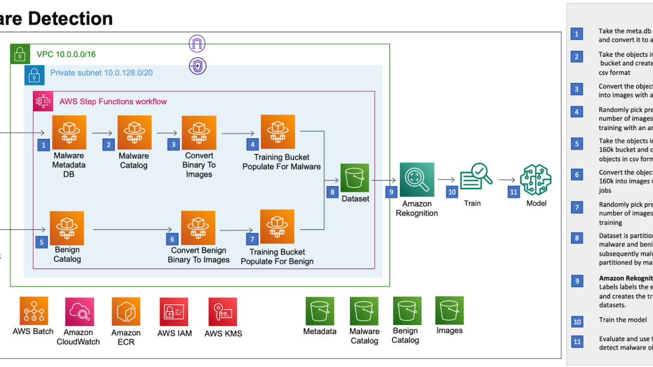
The following architecture diagram provides an overview of the solution.

The solution is built using AWS Batch, AWS Fargate, and Amazon Rekognition. AWS Batch lets you run hundreds of batch computing jobs on Fargate. Fargate is compatible with both Amazon Elastic Container Service (Amazon ECS) and Amazon Elastic Kubernetes Service (Amazon EKS). Amazon Rekognition custom labels lets you use AutoML for computer vision to train custom models to detect malware and classify various malware categories. AWS Step Functions are used to orchestrate data preprocessing.

For this solution, we create the preprocessing resources via AWS CloudFormation. The CloudFormation stack template and the source code for the AWS Batch, Fargate, and Step functions are available in a GitHub Repository.

Dataset

To train the model in this example, we used the following public datasets to extract the malicious and benign Portable Executable (PE):

• Sophos/ReversingLabs 20 Million malware detection dataset provides an extensive data set of malware objects from 11 different families. Since the dataset already exists on Amazon Simple Storage Service (Amazon S3), it’s relatively simple to embed it in the preprocessing flow.
• We source the benign objects through PE Malware Machine Learning Dataset, created and owned by Michael Lester. If you plan to use the same dataset, then first you will manually download the dataset and upload the binaries into an S3 bucket (i.e., benign-160k) which feeds the preprocessing flow.

We encourage you to read carefully through the datasets documentation (Sophos/Reversing Labs README, PE Malware Machine Learning Dataset) to safely handle the malware objects. Based on your preference, you can also use other datasets as long as they provide malware and benign objects in the binary format.

Next, we’ll walk you through the following steps of the solution:

• Preprocess objects and convert to images
• Deploy preprocessing resources with CloudFormation
• Choose the model
• Train the model
• Evaluate the model
• Cost and performance

Preprocess objects and convert to images

We use Step Functions to orchestrate the object preprocessing workflow which includes the following steps:

1. Take the meta.db sqllite database from sorel-20m S3 bucket and convert it to a .csv file. This helps us load the .csv file in a Fargate container and refer to the metadata while processing the malware objects.
2. Take the objects from the sorel-20m S3 bucket and create a list of objects in the csv format. By performing this step, we’re creating a series of .csv files which can be processed in parallel, thereby reducing the time taken for the preprocessing.
3. Convert the objects from the sorel-20m S3 bucket into images with an array of jobs. AWS Batch array jobs share common parameters for converting the malware objects into images. They run as a collection of image conversion jobs that are distributed across multiple hosts, and run concurrently.
4. Pick a predetermined number of images for the model training with an array of jobs corresponding to the categories of malware.
5. Similar to Step 2, we take the benign objects from the benign-160k S3 bucket and create a list of objects in csv format.
6. Similar to Step 3, we convert the objects from the benign-160k S3 bucket into images with an array of jobs.
7. Due to the Amazon Rekognition default quota for custom labels training (250K images), pick a predetermined number of benign images for the model training.
8. As shown in the following image, the images are stored in an S3 bucket partitioned first by malware and benign folders, and then subsequently the malware is partitioned by malware types.
   
   

Deploy the preprocessing resources with CloudFormation

Prerequisites

The following prerequisites are required before continuing:

• An AWS Account
• AWS Command Line Interface (AWS CLI)
• Python
• Docker
• AWS SDK for Python
• Amazon S3 Buckets that contain benign objects and their metadata database
• Amazon S3 Buckets that contain artifacts

Resource deployment

The CloudFormation stack will create the following resources:

• An Amazon Virtual Private Cloud (Amazon VPC)
• Public and Private Subnets
• Internet Gateway
• Nat Gateway
• AWS Batch Compute Environment
• AWS Batch Queues
• AWS Batch Job Definitions
• AWS Step Functions
• Amazon S3 Buckets
• AWS Key Management Service (AWS KMS) key
• AWS Identity and Access Management (IAM) roles and policies
• Amazon CloudWatch Logs Group

Parameters

• STACK_NAME – CloudFormation stack name
• AWS_REGION – AWS region where the solution will be deployed
• AWS_PROFILE – Named profile that will apply to the AWS CLI command
• ARTEFACT_S3_BUCKET – S3 bucket where the infrastructure code will be stored. (The bucket must be created in the same region where the solution lives).
• AWS_ACCOUNT – AWS Account ID.

Use the following commands to deploy the resources

Make sure the docker agent is running on the machine. The deployments are done using bash scripts, and in this case we use the following command:

bash malware_detection_deployment_scripts/deploy.sh -s '<STACK_NAME>' -b 'malware-
detection-<ACCOUNT_ID>-artifacts' -p <AWS_PROFILE> -r "<AWS_REGION>" -a
<ACCOUNT_ID>

This builds and deploys the local artifacts that the CloudFormation template (e.g., cloudformation.yaml) is referencing.

Train the model

Since Amazon Rekognition takes care of model training for you, computer vision or highly specialized ML knowledge isn’t required. However, you will need to provide Amazon Rekognition with a bucket filled with appropriately labeled input images.

In this post, we’ll train two independent image classification models via the custom labels feature:

1. Malware detection model (binary classification) – identify if the given object is malicious or benign
2. Malware classification model (multi-class classification) – identify the malware family for a given malicious object

Model training walkthrough

The steps listed in the following walkthrough apply to both models. Therefore, you will need to go through the steps two times in order to train both models.

1. Sign in to the AWS Management Console and open the Amazon Rekognition console.
2. In the left pane, choose Use Custom Labels. The Amazon Rekognition Custom Labels landing page is shown.
3. From the Amazon Rekognition Custom Labels landing page, choose Get started.
4. In the left pane, Choose Projects.
5. Choose Create Project.
6. In Project name, enter a name for your project.
7. Choose Create project to create your project.
8. In the Projects page, choose the project to which you want to add a dataset. The details page for your project is displayed.
9. Choose Create dataset. The Create dataset page is shown.
10. In Starting configuration, choose Start with a single dataset to let Amazon Rekognition split the dataset to training and test. Note that you might end up with different test samples in each model training iteration, resulting in slightly different results and evaluation metrics.
11. Choose Import images from Amazon S3 bucket.
12. In S3 URI, enter the S3 bucket location and folder path. The same S3 bucket provided from the preprocessing step is used to create both datasets: Malware detection and Malware classification. The Malware detection dataset points to the root (i.e., s3://malware-detection-training-{account-id}-{region}/) of the S3 bucket, while the Malware classification dataset points to the malware folder (i.e., s3://malware-detection-training-{account-id}-{region}/malware) of the S3 bucket.
13. Choose Automatically attach labels to images based on the folder.
14. Choose Create Datasets. The datasets page for your project opens.
15. On the Train model page, choose Train model. The Amazon Resource Name (ARN) for your project should be in the Choose project edit box. If not, then enter the ARN for your project.
16. In the Do you want to train your model? dialog box, choose Train model.
17. After training completes, choose the model’s name. Training is finished when the model status is TRAINING_COMPLETED.
18. In the Models section, choose the Use model tab to start using the model.

For more details, check the Amazon Rekognition custom labels Getting started guide.

Evaluate the model

When the training models are complete, you can access the evaluation metrics by selecting Check metrics on the model page. Amazon Rekognition provides you with the following metrics: F1 score, average precision, and overall recall, which are commonly used to evaluate the performance of classification models. The latter are averaged metrics over the number of labels.

In the Per label performance section, you can find the values of these metrics per label. Additionally, to get the values for True Positive, False Positive, and False negative, select the View test results.

Malware detection model metrics

On the balanced dataset of 199,750 images with two labels (benign and malware), we received the following results:

• F1 score – 0.980
• Average precision – 0.980
• Overall recall – 0.980

Malware classification model metrics

On the balanced dataset of 130,609 images with 11 labels (11 malware families), we received the following results:

• F1 score – 0.921
• Average precision – 0.938
• Overall recall – 0.906

To assess whether the model is performing well, we recommend comparing its performance with other industry benchmarks which have been trained on the same (or at least similar) dataset. Unfortunately, at the time of writing of this post, there are no comparative bodies of research which solve this problem using the same technique and the same datasets. However, within the data science community, a model with an F1 score above 0.9 is considered to perform very well.

Cost and performance

Due to the serverless nature of the resources, the overall cost is influenced by the amount of time that each service is used. On the other hand, performance is impacted by the amount of data being processed and the training dataset size feed to Amazon Rekognition. For our cost and performance estimate exercise, we consider the following scenario:

• 20 million objects are cataloged and processed from the sorel dataset.
• 160,000 objects are cataloged and processed from the PE Malware Machine Learning Dataset.
• Approximately 240,000 objects are written to the training S3 bucket: 160,000 malware objects and 80,000 benign objects.

Based on this scenario, the average cost to preprocess and deploy the models is $510.99 USD. You will be charged additionally $4 USD/h for every hour that you use the model. You may find the detailed cost breakdown in the estimate generated via the AWS Pricing Calculator.

Performance-wise, these are the results from our measurement:

• ~2 h for the preprocessing flow to complete
• ~40 h for the malware detecting model training to complete
• ~40 h for the malware classification model training to complete

Clean-up

To avoid incurring future charges, stop and delete the Amazon Rekognition models, and delete the preprocessing resources via the destroy.sh script. The following parameters are required to run the script successfully:

• STACK_NAME – The CloudFormation stack name
• AWS_REGION – The Region where the solution is deployed
• AWS_PROFILE – The named profile that applies to the AWS CLI command

Use the following commands to run the ./malware_detection_deployment_scripts/destroy.sh script:

bash malware_detection_deployment_scripts/destroy.sh -s <STACK_NAME> -p
<AWS_PROFILE> -r <AWS_REGION>

Conclusion

In this post, we demonstrated how to perform malware detection and classification using Amazon Rekognition. The solutions follow a serverless pattern, leveraging managed services for data preprocessing, orchestration, and model deployment. We hope that this post helps you in your ongoing efforts to combat malware.

In a future post we’ll show a practical use case of malware detection by consuming the models deployed in this post.

About the authors

Edvin Hallvaxhiu is a Senior Global Security Architect with AWS Professional Services and is passionate about cybersecurity and automation. He helps customers build secure and compliant solutions in the cloud. Outside work, he likes traveling and sports.

Rahul Shaurya is a Principal Data Architect with AWS Professional Services. He helps and works closely with customers building data platforms and analytical applications on AWS. Outside of work, Rahul loves taking long walks with his dog Barney.

Bruno Dhefto is a Global Security Architect with AWS Professional Services. He is focused on helping customers building Secure and Reliable architectures in AWS. Outside of work, he is interested in the latest technology updates and traveling.

Nadim Majed is a data architect within AWS professional services. He works side by side with customers building their data platforms on AWS. Outside work, Nadim plays table tennis, and loves watching football/soccer.

Read More

Data is transforming every field and every business. However, with data growing faster than most companies can keep track of, collecting data and getting value out of that data is a challenging thing to do. A modern data strategy can help you create better business outcomes with data. AWS provides the most complete set of services for the end-to-end data journey to help you unlock value from your data and turn it into insight.

Data scientists can spend up to 80% of their time preparing data for machine learning (ML) projects. This preparation process is largely undifferentiated and tedious work, and can involve multiple programming APIs and custom libraries. Amazon SageMaker Data Wrangler helps data scientists and data engineers simplify and accelerate tabular and time series data preparation and feature engineering through a visual interface. You can import data from multiple data sources, such as Amazon Simple Storage Service (Amazon S3), Amazon Athena, Amazon Redshift, or even third-party solutions like Snowflake or DataBricks, and process your data with over 300 built-in data transformations and a library of code snippets, so you can quickly normalize, transform, and combine features without writing any code. You can also bring your custom transformations in PySpark, SQL, or Pandas.

This post demonstrates how you can schedule your data preparation jobs to run automatically. We also explore the new Data Wrangler capability of parameterized datasets, which allows you to specify the files to be included in a data flow by means of parameterized URIs.

Solution overview

Data Wrangler now supports importing data using a parameterized URI. This allows for further flexibility because you can now import all datasets matching the specified parameters, which can be of type String, Number, Datetime, and Pattern, in the URI. Additionally, you can now trigger your Data Wrangler transformation jobs on a schedule.

In this post, we create a sample flow with the Titanic dataset to show how you can start experimenting with these two new Data Wrangler’s features. To download the dataset, refer to Titanic – Machine Learning from Disaster.

Prerequisites

To get all the features described in this post, you need to be running the latest kernel version of Data Wrangler. For more information, refer to Update Data Wrangler. Additionally, you need to be running Amazon SageMaker Studio JupyterLab 3. To view the current version and update it, refer to JupyterLab Versioning.

File structure

For this demonstration, we follow a simple file structure that you must replicate in order to reproduce the steps outlined in this post.

1. In Studio, create a new notebook.
2. Run the following code snippet to create the folder structure that we use (make sure you’re in the desired folder in your file tree):

   !mkdir titanic_dataset
   !mkdir titanic_dataset/datetime_data
   !mkdir titanic_dataset/datetime_data/2021
   !mkdir titanic_dataset/datetime_data/2022
   
   !mkdir titanic_dataset/datetime_data/2021/01 titanic_dataset/datetime_data/2021/02 titanic_dataset/datetime_data/2021/03 
   !mkdir titanic_dataset/datetime_data/2021/04 titanic_dataset/datetime_data/2021/05 titanic_dataset/datetime_data/2021/06
   !mkdir titanic_dataset/datetime_data/2022/01 titanic_dataset/datetime_data/2022/02 titanic_dataset/datetime_data/2022/03 
   !mkdir titanic_dataset/datetime_data/2022/04 titanic_dataset/datetime_data/2022/05 titanic_dataset/datetime_data/2022/06
   
   !mkdir titanic_dataset/datetime_data/2021/01/01 titanic_dataset/datetime_data/2021/02/01 titanic_dataset/datetime_data/2021/03/01 
   !mkdir titanic_dataset/datetime_data/2021/04/01 titanic_dataset/datetime_data/2021/05/01 titanic_dataset/datetime_data/2021/06/01
   !mkdir titanic_dataset/datetime_data/2022/01/01 titanic_dataset/datetime_data/2022/02/01 titanic_dataset/datetime_data/2022/03/01 
   !mkdir titanic_dataset/datetime_data/2022/04/01 titanic_dataset/datetime_data/2022/05/01 titanic_dataset/datetime_data/2022/06/01
   
   !mkdir titanic_dataset/train_1 titanic_dataset/train_2 titanic_dataset/train_3 titanic_dataset/train_4 titanic_dataset/train_5
   !mkdir titanic_dataset/train titanic_dataset/test

3. Copy the train.csv and test.csv files from the original Titanic dataset to the folders titanic_dataset/train and titanic_dataset/test, respectively.
4. Run the following code snippet to populate the folders with the necessary files:

   import os
   import math
   import pandas as pd
   batch_size = 100
   
   #Get a list of all the leaf nodes in the folder structure
   leaf_nodes = []
   
   for root, dirs, files in os.walk('titanic_dataset'):
       if not dirs:
           if root != "titanic_dataset/test" and root != "titanic_dataset/train":
               leaf_nodes.append(root)
               
   titanic_df = pd.read_csv('titanic_dataset/train/train.csv')
   
   #Create the mini batch files
   for i in range(math.ceil(titanic_df.shape[0]/batch_size)):
       batch_df = titanic_df[i*batch_size:(i+1)*batch_size]
       
       #Place a copy of each mini batch in each one of the leaf folders
       for node in leaf_nodes:
           batch_df.to_csv(node+'/part_{}.csv'.format(i), index=False)

We split the train.csv file of the Titanic dataset into nine different files, named part_x, where x is the number of the part. Part 0 has the first 100 records, part 1 the next 100, and so on until part 8. Every node folder of the file tree contains a copy of the nine parts of the training data except for the train and test folders, which contain train.csv and test.csv.

Parameterized datasets

Data Wrangler users can now specify parameters for the datasets imported from Amazon S3. Dataset parameters are specified at the resources’ URI, and its value can be changed dynamically, allowing for more flexibility for selecting the files that we want to import. Parameters can be of four data types:

• Number – Can take the value of any integer
• String – Can take the value of any text string
• Pattern – Can take the value of any regular expression
• Datetime – Can take the value of any of the supported date/time formats

In this section, we provide a walkthrough of this new feature. This is available only after you import your dataset to your current flow and only for datasets imported from Amazon S3.

1. From your data flow, choose the plus (+) sign next to the import step and choose Edit dataset.
2. The preferred (and easiest) method of creating new parameters is by highlighting a section of you URI and choosing Create custom parameter on the drop-down menu. You need to specify four things for each parameter you want to create:
   1. Name
   2. Type
   3. Default value
   4. Description

   
   Here we have created a String type parameter called filename_param with a default value of train.csv. Now you can see the parameter name enclosed in double brackets, replacing the portion of the URI that we previously highlighted. Because the defined value for this parameter was train.csv, we now see the file train.csv listed on the import table.
   

3. When we try to create a transformation job, on the Configure job step, we now see a Parameters section, where we can see a list of all of our defined parameters.
4. Choosing the parameter gives us the option to change the parameter’s value, in this case, changing the input dataset to be transformed according to the defined flow.
   Assuming we change the value of filename_param from train.csv to part_0.csv, the transformation job now takes part_0.csv (provided that a file with the name part_0.csv exists under the same folder) as its new input data.
   
5. Additionally, if you attempt to export your flow to an Amazon S3 destination (via a Jupyter notebook), you now see a new cell containing the parameters that you defined.
   Note that the parameter takes their default value, but you can change it by replacing its value in the parameter_overrides dictionary (while leaving the keys of the dictionary unchanged).
   
   Additionally, you can create new parameters from the Parameters UI.
6. Open it up by choosing the parameters icon ({{}}) located next to the Go option; both of them are located next to the URI path value.
   A table opens with all the parameters that currently exist on your flow file (filename_param at this point).
7. You can create new parameters for your flow by choosing Create Parameter.
   
   A pop-up window opens to let you create a new custom parameter.
8. Here, we have created a new example_parameter as Number type with a default value of 0. This newly created parameter is now listed in the Parameters table. Hovering over the parameter displays the options Edit, Delete, and Insert.
9. From within the Parameters UI, you can insert one of your parameters to the URI by selecting the desired parameter and choosing Insert.
   This adds the parameter to the end of your URI. You need to move it to the desired section within your URI.
   
10. Change the parameter’s default value, apply the change (from the modal), choose Go, and choose the refresh icon to update the preview list using the selected dataset based on the newly defined parameter’s value.Let’s now explore other parameter types. Assume we now have a dataset split into multiple parts, where each file has a part number.
11. If we want to dynamically change the file number, we can define a Number parameter as shown in the following screenshot.Note that the selected file is the one that matches the number specified in the parameter.
    Now let’s demonstrate how to use a Pattern parameter. Suppose we want to import all the part_1.csv files in all of the folders under the titanic-dataset/ folder. Pattern parameters can take any valid regular expression; there are some regex patterns shown as examples.
12. Create a Pattern parameter called any_pattern to match any folder or file under the titanic-dataset/ folder with default value .*.Notice that the wildcard is not a single * (asterisk) but also has a dot.
13. Highlight the titanic-dataset/ part of the path and create a custom parameter. This time we choose the Pattern type.This pattern selects all the files called part-1.csv from any of the folders under titanic-dataset/.
    A parameter can be used more than once in a path. In the following example, we use our newly created parameter any_pattern twice in our URI to match any of the part files in any of the folders under titanic-dataset/.
    Finally, let’s create a Datetime parameter. Datetime parameters are useful when we’re dealing with paths that are partitioned by date and time, like those generated by Amazon Kinesis Data Firehose (see Dynamic Partitioning in Kinesis Data Firehose). For this demonstration, we use the data under the datetime-data folder.
14. Select the portion of your path that is a date/time and create a custom parameter. Choose the Datetime parameter type.
    When choosing the Datetime data type, you need to fill in more details.
15. First of all, you must provide a date format. You can choose any of the predefined date/time formats or create a custom one.
    For the predefined date/time formats, the legend provides an example of a date matching the selected format. For this demonstration, we choose the format yyyy/MM/dd.
16. Next, specify a time zone for the date/time values.
    For example, the current date may be January 1, 2022, in one time zone, but may be January 2, 2022, in another time zone.
17. Finally, you can select the time range, which lets you select the range of files that you want to include in your data flow.
    You can specify your time range in hours, days, weeks, months, or years. For this example, we want to get all the files from the last year.
18. Provide a description of the parameter and choose Create.
    If you’re using multiple datasets with different time zones, the time is not converted automatically; you need to preprocess each file or source to convert it to one time zone.The selected files are all the files under the folders corresponding to last year’s data.
19. Now if we create a data transformation job, we can see a list of all of our defined parameters, and we can override their default values so that our transformation jobs pick the specified files.
    

Schedule processing jobs

You can now schedule processing jobs to automate running the data transformation jobs and exporting your transformed data to either Amazon S3 or Amazon SageMaker Feature Store. You can schedule the jobs with the time and periodicity that suits your needs.

Scheduled processing jobs use Amazon EventBridge rules to schedule the job’s run. Therefore, as a prerequisite, you have to make sure that the AWS Identity and Access Management (IAM) role being used by Data Wrangler, namely the Amazon SageMaker execution role of the Studio instance, has permissions to create EventBridge rules.

Configure IAM

Proceed with the following updates on the IAM SageMaker execution role corresponding to the Studio instance where the Data Wrangler flow is running:

1. Attach the AmazonEventBridgeFullAccess managed policy.
2. Attach a policy to grant permission to create a processing job:

   {
   	"Version": "2012-10-17",
   	"Statement": [
   		{
   			"Effect": "Allow",
   			"Action": "sagemaker:StartPipelineExecution",
   			"Resource": "arn:aws:sagemaker:Region:AWS-account-id:pipeline/data-wrangler-*"
   		}
   	]
   }

3. Grant EventBridge permission to assume the role by adding the following trust policy:

   {
   	"Effect": "Allow",
   	"Principal": {
   		"Service": "events.amazonaws.com"
   	},
   	"Action": "sts:AssumeRole"
   }

Alternatively, if you’re using a different role to run the processing job, apply the policies outlined in steps 2 and 3 to that role. For details about the IAM configuration, refer to Create a Schedule to Automatically Process New Data.

Create a schedule

To create a schedule, have your flow opened in the Data Wrangler flow editor.

1. On the Data Flow tab, choose Create job.
2. Configure the required fields and chose Next, 2. Configure job.
   
3. Expand Associate Schedules.
4. Choose Create new schedule.
   
   The Create new schedule dialog opens, where you define the details of the processing job schedule.
   The dialog offers great flexibility to help you define the schedule. You can have, for example, the processing job running at a specific time or every X hours, on specific days of the week.
   The periodicity can be granular to the level of minutes.
5. Define the schedule name and periodicity, then choose Create to save the schedule.
6. You have the option to start the processing job right away along with the scheduling, which takes care of future runs, or leave the job to run only according to the schedule.
7. You can also define an additional schedule for the same processing job.
   
8. To finish the schedule for the processing job, choose Create.
   You see a “Job scheduled successfully” message. Additionally, if you chose to leave the job to run only according to the schedule, you see a link to the EventBridge rule that you just created.

If you choose the schedule link, a new tab in the browser opens, showing the EventBridge rule. On this page, you can make further modifications to the rule and track its invocation history. To stop your scheduled processing job from running, delete the event rule that contains the schedule name.

The EventBridge rule shows a SageMaker pipeline as its target, which is triggered according to the defined schedule, and the processing job invoked as part of the pipeline.

To track the runs of the SageMaker pipeline, you can go back to Studio, choose the SageMaker resources icon, choose Pipelines, and choose the pipeline name you want to track. You can now see a table with all current and past runs and status of that pipeline.

You can see more details by double-clicking a specific entry.

Clean up

When you’re not using Data Wrangler, it’s recommended to shut down the instance on which it runs to avoid incurring additional fees.

To avoid losing work, save your data flow before shutting Data Wrangler down.

1. To save your data flow in Studio, choose File, then choose Save Data Wrangler Flow. Data Wrangler automatically saves your data flow every 60 seconds.
2. To shut down the Data Wrangler instance, in Studio, choose Running Instances and Kernels.
3. Under RUNNING APPS, choose the shutdown icon next to the sagemaker-data-wrangler-1.0 app.
4. Choose Shut down all to confirm.

Data Wrangler runs on an ml.m5.4xlarge instance. This instance disappears from RUNNING INSTANCES when you shut down the Data Wrangler app.

After you shut down the Data Wrangler app, it has to restart the next time you open a Data Wrangler flow file. This can take a few minutes.

Conclusion

In this post, we demonstrated how you can use parameters to import your datasets using Data Wrangler flows and create data transformation jobs on them. Parameterized datasets allow for more flexibility on the datasets you use and allow you to reuse your flows. We also demonstrated how you can set up scheduled jobs to automate your data transformations and exports to either Amazon S3 or Feature Store, at the time and periodicity that suits your needs, directly from within Data Wrangler’s user interface.

To learn more about using data flows with Data Wrangler, refer to Create and Use a Data Wrangler Flow and Amazon SageMaker Pricing. To get started with Data Wrangler, see Prepare ML Data with Amazon SageMaker Data Wrangler.

About the authors

David Laredo is a Prototyping Architect for the Prototyping and Cloud Engineering team at Amazon Web Services, where he has helped develop multiple machine learning prototypes for AWS customers. He has been working in machine learning for the last 6 years, training and fine-tuning ML models and implementing end-to-end pipelines to productionize those models. His areas of interest are NLP, ML applications, and end-to-end ML.

Givanildo Alves is a Prototyping Architect with the Prototyping and Cloud Engineering team at Amazon Web Services, helping clients innovate and accelerate by showing the art of possible on AWS, having already implemented several prototypes around artificial intelligence. He has a long career in software engineering and previously worked as a Software Development Engineer at Amazon.com.br.

Adrian Fuentes is a Program Manager with the Prototyping and Cloud Engineering team at Amazon Web Services, innovating for customers in machine learning, IoT, and blockchain. He has over 15 years of experience managing and implementing projects and 1 year of tenure on AWS.

Read More

In machine learning (ML), data quality has direct impact on model quality. This is why data scientists and data engineers spend significant amount of time perfecting training datasets. Nevertheless, no dataset is perfect—there are trade-offs to the preprocessing techniques such as oversampling, normalization, and imputation. Also, mistakes and errors could creep in at various stages of data analytics pipeline.

In this post, you will learn how to use built-in analysis types in Amazon SageMaker Data Wrangler to help you detect the three most common data quality issues: multicollinearity, target leakage, and feature correlation.

Data Wrangler is a feature of Amazon SageMaker Studio which provides an end-to-end solution for importing, preparing, transforming, featurizing, and analyzing data. The transformation recipes created by Data Wrangler can integrate easily into your ML workflows and help streamline data preprocessing as well as feature engineering using little to no coding. You can also add your own Python scripts and transformations to customize the recipes.

Solution overview

To demonstrate Data Wrangler’s functionality in this post we are going to use the popular Titanic dataset. The dataset describes the survival status of individual passengers on the Titanic and has 14 columns, including the target column. These features include pclass, name, survived, age, embarked, home. dest, room, ticket, boat, and sex. The column pclass refers to passenger class (1st, 2nd, 3rd), and is a proxy for socio-economic class. The column survived is the target column.

Prerequisites

To use Data Wrangler, you need an active Studio instance. To learn how to launch a new instance, see Onboard to Amazon SageMaker Domain.

Before you get started, download the Titanic dataset to an Amazon Simple Storage Service (Amazon S3) bucket.

Create a data flow

To access Data Wrangler in Studio, complete the following steps:

1. Next to the user you want to use to launch Studio, choose Open Studio.
2. When Studio opens, choose the plus sign on the New data flow card under ML tasks and components.

This creates a new directory in Studio with a .flow file inside, which contains your data flow. The .flow file automatically opens in Studio.

You can also create a new flow by choosing File, then New, and choosing Data Wrangler Flow.

3. Optionally, rename the new directory and the .flow file.

When you create a new .flow file in Studio, you might see a carousel that introduces you to Data Wrangler. This may take a few minutes.

When the Data Wrangler instance is active, you can see the data flow screen as shown in the following screenshot.

4. Choose Use sample dataset to load the titanic dataset.

Create a Quick Model analysis

There are two ways to get a sense for a new (previously unseen) dataset. One is to run Data Quality and Insights Report. This report will provide high level statistics – number features, rows, missing values, etc and surface high priority warnings (if present) – duplicate rows, target leakage, anomalous samples, etc.

Another way is to run Quick Model analysis directly. Complete the following steps:

1. Choose the plus sign and choose Add analysis.

2. For Analysis type, choose Quick Model.
3. For Analysis name¸ enter a name.
4. For Label, choose the target label from the list of your feature columns (Survived).
5. Choose Save.

The following graph visualizes our findings.

Quick Model trains a random forest with 10 trees on 730 observations and measures prediction quality on the remaining 315 observations. The dataset is automatically sampled and split into training and validation tests (70:30). In this example, you can see that the model achieved an F1 score of 0.777 on the test set. This could be an indicator that the data you’re exploring has the potential of being predictive.

At the same time, a few things stand out right away. The columns name and boat are the highest contributing signals towards your prediction. String columns like name can be both useful and not useful depending on the comprehensive information they carry about the person, like first, middle, and last names alongside the historical time periods and trends they belong to. This column can either be excluded or retained depending on the outcome of the contribution. In this case, a simple preview reveals that passenger names also include their titles (Mr, Dr, etc) which could potentially carry valuable information; therefore, we’re going to keep it. However, we do want to take a closer look at the boat column, which also seems to have a strong predictive power.

Target leakage

First, let’s start with the concept of leakage. Leakage can occur during different stages of the ML lifecycle. Using features that are available only during training but not during inference can also be defined as target leakage. For example, a deployed airbag is not a good predictor for a car crash, because in real life it occurs after the fact.

One of the techniques for identifying target leakage relies on computing ROC values for each feature. The closer the value is to a 1, the more likely the feature is very predictive of the target and therefore the more likely it’s a leaked target. On the other hand, the closer the value is to 0.5 and below (rarely), the less likely this feature contributes anything towards prediction. Finally, values that are above 0.5 and below 1 indicate that the feature doesn’t carry predictive power by itself, but may be a contributor in a group—which is what we’d like to see ideally.

Let’s create a target leakage analysis on your dataset. This analysis together with a set of advanced analyses are offered as built-in analysis types in Data Wrangler. To create the analysis, choose Add Analysis and choose Target Leakage. This is similar to how you previously created a Quick Model analysis.

As you can see in the following figure, your most predictive feature boat is quite close in ROC value to 1, which makes it a possible suspect for target leakage.

If you read the description of the dataset, the boat column contains the lifeboat number in which the passenger managed to escape. Naturally, there is quite a close correlation with the survival label. The lifeboat number is known only after the fact—when the lifeboat was picked up and the survivors on it were identified. This is very similar to the airbag example. Therefore, the boat column is indeed a target leakage.

You can eliminate it from your dataset by applying the drop column transform in the Data Wrangler UI (choose Handle Columns, choose Drop, and indicate boat). Now if you rerun the analysis, you get the following.

Multicollinearity

Multicollinearity occurs when two or more features in a dataset are highly correlated with one another. Detecting the presence of multicollinearity in a dataset is important because multicollinearity can reduce predictive capabilities of an ML model. Multicollinearity can either already be present in raw data received from an upstream system, or it can be inadvertently introduced during feature engineering. For instance, the Titanic dataset contains two columns indicating the number of family members each passenger traveled with: number of siblings (sibsp) and number of parents (parch). Let’s say that somewhere in your feature engineering pipeline, you decided that it would make sense to introduce a simpler measure of each passenger’s family size by combining the two.

A very simple transformation step can help us achieve that, as shown in the following screenshot.

As a result, you now have a column called family_size, which reflects just that. If you didn’t drop the original two columns, you now have very strong correlation between both siblings as well as the parents columns and the family size. By creating another analysis and choosing Multicollinearity, you can now see the following.

In this case, you’re using the Variance Inflation Factor (VIF) approach to identify highly correlated features. VIF scores are calculated by solving a regression problem to predict one variable given the rest, and they can range between 1 and infinity. The higher the value is, the more dependent a feature is. Data Wrangler’s implementation of VIF analysis caps the scores at 50 and in general, a score of 5 means the feature is moderately correlated, whereas anything above 5 is considered highly correlated.

Your newly engineered feature is highly dependent on the original columns, which you can now simply drop by using another transformation by choosing Manage Columns, Drop Column.

An alternative approach to identify features that have less or more predictive power is to use the Lasso feature selection type of the multicollinearity analysis (for Problem type, choose Classification and for Label column, choose survived).

As outlined in the description, this analysis builds a linear classifier that provides a coefficient for each feature. The absolute value of this coefficient can also be interpreted as the importance score for the feature. As you can observe in your case, family_size carries no value in terms of feature importance due to its redundancy, unless you drop the original columns.

After dropping sibsp and parch, you get the following.

Data Wrangler also provides a third option to detect multicollinearity in your dataset facilitated via Principal Component Analysis (PCA). PCA measures the variance of the data along different directions in the feature space. The ordered list of variances, also known as the singular values, can inform about multicollinearity in your data. This list contains non-negative numbers. When the numbers are roughly uniform, the data has very few multicollinearities. However, when the opposite is true, the magnitude of the top values will dominate the rest. To avoid issues related to different scales, the individual features are standardized to have mean 0 and standard deviation 1 before applying PCA.

Before dropping the original columns (sibsp and parch), your PCA analysis is shown as follows.

After dropping sibsp and parch, you have the following.

Feature correlation

Correlation is a measure of the degree of dependence between variables. Correlated features in general don’t improve models but can have an impact on models. There are two types of correlation detection features available in Data Wrangler: linear and non-linear.

Linear feature correlation is based on Pearson’s correlation. Numeric-to-numeric correlation is in the range [-1, 1] where 0 implies no correlation, 1 implies perfect correlation, and -1 implies perfect inverse correlation. Numeric-to-categorical and categorical-to-categorical correlations are in the range [0, 1] where 0 implies no correlation and 1 implies perfect correlation. Features that are not either numeric or categorical are ignored.

The following correlation matrix and score table validate and reinforce your previous findings.

The columns survived and boat are highly correlating with each other. For this example, survived is the target column or the label you’re trying to predict. You saw this previously in your target leakage analysis. On the other hand, columns sibsp and parch are highly correlating with the derived feature family_size. This was confirmed in your previous multicollinearity analysis. We don’t see any strong inverse linear correlation in the dataset.

When two variable changes in a constant proportion, it’s called a linear correlation, whereas when the two variables don’t change in any constant proportion, the relationship is non-linear. Correlation is perfectly positive when proportional change in two variables is in the same direction. In contrast, correlation is perfectly negative when proportional change in two variables is in the opposite direction.

The difference between feature correlation and multi-collinearity (discussed previously) is as follows: feature correlation refers to the linear or non-linear relationship between two variables. With this context, you can define collinearity as a problem where two or more independent variables (predictors) have a strong linear or non-linear relationship. Multicollinearity is a special case of collinearity where a strong linear relationship exists between three or more independent variables even if no pair of variables has a high correlation.

Non-linear feature correlation is based on Spearman’s rank correlation. Numeric-to-categorical correlation is calculated by encoding the categorical features as the floating-point numbers that best predict the numeric feature before calculating Spearman’s rank correlation. Categorical-to-categorical correlation is based on the normalized Cramer’s V test.

Numeric-to-numeric correlation is in the range [-1, 1] where 0 implies no correlation, 1 implies perfect correlation, and -1 implies perfect inverse correlation. Numeric-to-categorical and categorical-to-categorical correlations are in the range [0, 1] where 0 implies no correlation and 1 implies perfect correlation. Features that aren’t numeric or categorical are ignored.

The following table lists for each feature what is the most correlated feature to it. It displays a correlation matrix for a dataset with up to 20 columns.

The results are very similar to what you saw in the previous linear correlation analysis, except you can also see a strong negative non-linear correlation between the pclass and fare numeric columns.

Finally, now that you have identified potential target leakage and eliminated features based on your analyses, let’s rerun the Quick Model analysis to look at the feature importance breakdown again.

The results look quite different than what you started with initially. Therefore, Data Wrangler makes it easy to run advanced ML-specific analysis with a few clicks and derive insights about the relationship between your independent variables (features) among themselves and also with the target variable. It also provides you with the Quick Model analysis type that lets you validate the current state of features by training a quick model and testing how predictive the model is.

Ideally, as a data scientist, you should start with some of the analyses showcased in this post and derive insights into what features are good to retain vs. what to drop.

Summary

In this post, you learned how to use Data Wrangler for exploratory data analysis, focusing on target leakage, feature correlation, and multicollinearity analyses to identify potential issues with training data and mitigate them with the help of built-in transformations. As next steps, we recommend you replicate the example in this post in your Data Wrangler data flow to experience what was discussed here in action.

If you’re new to Data Wrangler or Studio, refer to Get Started with Data Wrangler. If you have any questions related to this post, please add it in the comments section.

About the authors

Vadim Omeltchenko is a Sr. AI/ML Solutions Architect who is passionate about helping AWS customers innovate in the cloud. His prior IT experience was predominantly on the ground.

Arunprasath Shankar is a Sr. AI/ML Specialist Solutions Architect with AWS, helping global customers scale their AI solutions effectively and efficiently in the cloud. In his spare time, Arun enjoys watching sci-fi movies and listening to classical music.

Read More

At AWS, we have been investing in healthcare since Day 1 with customers including Moderna, Rush University Medical Center, and the NHS who have built breakthrough innovations in the cloud. From developing public health analytics hubs, to improving health equity and patient outcomes, to developing a COVID-19 vaccine in just 65 days, our customers are utilizing machine learning (ML) and the cloud to address some of healthcare’s biggest challenges and drive change toward more predictive and personalized care.

Last year, we launched Amazon HealthLake, a purpose-built service to store, transform, and query health data in the cloud, allowing you to benefit from a complete view of individual or patient population health data at scale.

Today, we’re excited to announce the launch of two new capabilities in HealthLake that deliver innovations for medical imaging and analytics.

Amazon HealthLake Imaging

Healthcare professionals face a myriad of challenges as the scale and complexity of medical imaging data continues to increase including the following:

• The volume of medical imaging data has continued to accelerate over the past decade with over 5.5 billion imaging procedures done across the globe each year by a shrinking number of radiologists
• The average imaging study size has doubled over the past decade to 150 MB as more advanced imaging procedures are being performed due to improvements in resolution and the increasing use of volumetric imaging
• Health systems store multiple copies of the same imaging data in clinical and research systems, which leads to increased costs and complexity
• It can be difficult to structure this data, which often takes data scientists and researchers weeks or months to derive important insights with advanced analytics and ML

These compounding factors are slowing down decision-making, which can affect care delivery. To address these challenges, we are excited to announce the preview of Amazon HealthLake Imaging, a new HIPAA-eligible capability that makes it easy to store, access, and analyze medical images at petabyte scale. This new capability is designed for fast, sub-second  medical image retrieval in your clinical workflows that you can access securely from anywhere (e.g., web, desktop, phone) and with high availability. Additionally, you can drive your existing medical viewers and analysis applications from a single encrypted copy of the same data in the cloud with normalized metadata and advanced compression. As a result, it is estimated that HealthLake Imaging helps you reduce the total cost of medical imaging storage by up to 40%.

We are proud to be working with partners on the launch of HealthLake Imaging to accelerate adoption of cloud-native solutions to help transition enterprise imaging workflows to the cloud and accelerate your pace of innovation.

Intelerad and Arterys are among the launch partners utilizing HealthLake Imaging to achieve higher scalability and viewing performance for their next-generation PACS systems and AI platform, respectively. Radical Imaging is providing customers with zero-footprint, cloud-capable medical imaging applications using open-source projects, such as OHIF or Cornerstone.js, built on HealthLake Imaging APIs. And NVIDIA has collaborated with AWS to develop a MONAI connector for HealthLake Imaging. MONAI is an open-source medical AI framework to develop and deploy models into AI applications, at scale.

“Intelerad has always focused on solving complex problems in healthcare, while enabling our customers to grow and provide exceptional patient care to more patients around the globe. In our continuous path of innovation, our collaboration with AWS, including leveraging Amazon HealthLake Imaging, allows us to innovate more quickly and reduce complexity while offering unparalleled scale and performance for our users.”

— AJ Watson, Chief Product Officer at Intelerad Medical Systems

“With Amazon HealthLake Imaging, Arterys was able to achieve noticeable improvements in performance and responsiveness of our applications, and with a rich feature set of future-looking enhancements, offers benefits and value that will enhance solutions looking to drive future-looking value out of imaging data.”

— Richard Moss, Director of Product Management at Arterys

Radboudumc and the University of Maryland Medical Intelligent Imaging Center (UM2ii) are among the customers utilizing HealthLake Imaging to improve the availability of medical images and utilize image streaming.

“At Radboud University Medical Center, our mission is to be a pioneer in shaping a more person-centered, innovative future of healthcare. We are building a collaborative AI solution with Amazon HealthLake Imaging for clinicians and researchers to speed up innovation by putting ML algorithms into the hands of clinicians faster.”

— Bram van Ginneken, Chair, Diagnostic Image Analysis Group at Radboudumc

“UM2ii was formed to unite innovators, thought leaders, and scientists across academics and industry. Our work with AWS will accelerate our mission to push the boundaries of medical imaging AI. We are excited to build the next generation of cloud-based intelligent imaging with Amazon HealthLake Imaging and AWS’s experience with scalability, performance, and reliability.”

— Paul Yi, Director at UM2ii

Amazon HealthLake Analytics

The second capability we’re excited to announce is Amazon HealthLake Analytics. Harnessing multi-modal data, which is highly contextual and complex, is key to making meaningful progress in providing patients highly personalized and precisely targeted diagnostics and treatments.

HealthLake Analytics makes it easy to query and derive insights from multi-modal health data at scale, at the individual or population levels, with the ability to share data securely across the enterprise and enable advanced analytics and ML in just a few clicks. This removes the need for you to execute complex data exports and data transformations.

HealthLake Analytics automatically normalizes raw health data from multiple disparate sources (e.g. medical records, health insurance claims, EHRs, medical devices) into an analytics and interoperability-ready format in a matter of minutes. Integration with other AWS services makes it easy to query the data with SQL using Amazon Athena, as well as share and analyze data to enable advanced analytics and ML. You can create powerful dashboards with Amazon QuickSight for care gap analyses and disease management of an entire patient population. Or you can build and train many ML models quickly and efficiently in Amazon SageMaker for AI-driven predictions, such as risk of hospital readmission or overall effectiveness of a line of treatment. HealthLake Analytics reduces what would take months of engineering effort and allows you to do what you do best—deliver care for patients.

Conclusion

At AWS, our goal is to support you to deliver convenient, personalized, and high-value care – helping you to reinvent how you collaborate, make data-driven clinical and operational decisions, enable precision medicine, accelerate therapy development, and decrease the cost of care.

With these new capabilities in Amazon HealthLake, we along with our partners can help enable next-generation imaging workflows in the cloud and derive insights from multi-modal health data, while complying with HIPAA, GDPR, and other regulations.

To learn more and get started, refer to Amazon HealthLake Analytics and Amazon HealthLake Imaging.

About the authors

Tehsin Syed is General Manager of Health AI at Amazon Web Services, and leads our Health AI engineering and product development efforts including Amazon Comprehend Medical and Amazon Health. Tehsin works with teams across Amazon Web Services responsible for engineering, science, product and technology to develop ground breaking healthcare and life science AI solutions and products. Prior to his work at AWS, Tehsin was Vice President of engineering at Cerner Corporation where he spent 23 years at the intersection of healthcare and technology.

Dr. Taha Kass-Hout is Vice President, Machine Learning, and Chief Medical Officer at Amazon Web Services, and leads our Health AI strategy and efforts, including Amazon Comprehend Medical and Amazon HealthLake. He works with teams at Amazon responsible for developing the science, technology, and scale for COVID-19 lab testing, including Amazon’s first FDA authorization for testing our associates—now offered to the public for at-home testing. A physician and bioinformatician, Taha served two terms under President Obama, including the first Chief Health Informatics officer at the FDA. During this time as a public servant, he pioneered the use of emerging technologies and the cloud (the CDC’s electronic disease surveillance), and established widely accessible global data sharing platforms: the openFDA, which enabled researchers and the public to search and analyze adverse event data, and precisionFDA (part of the Presidential Precision Medicine initiative).

Read More

Amazon SageMaker Data Wrangler helps you understand, aggregate, transform, and prepare data for machine learning (ML) from a single visual interface. It contains over 300 built-in data transformations so you can quickly normalize, transform, and combine features without having to write any code.

Data science practitioners generate, observe, and process data to solve business problems where they need to transform and extract features from datasets. Transforms such as ordinal encoding or one-hot encoding learn encodings on your dataset. These encoded outputs are referred as trained parameters. As datasets change over time, it may be necessary to refit encodings on previously unseen data to keep the transformation flow relevant to your data.

We are excited to announce the refit trained parameter feature, which allows you to use previous trained parameters and refit them as desired. In this post, we demonstrate how to use this feature.

Overview of the Data Wrangler refit feature

We illustrate how this feature works with the following example, before we dive into the specifics of the refit trained parameter feature.

Assume your customer dataset has a categorical feature for country represented as strings like Australia and Singapore. ML algorithms require numeric inputs; therefore, these categorical values have to be encoded to numeric values. Encoding categorical data is the process of creating a numerical representation for categories. For example, if your category country has values Australia and Singapore, you may encode this information into two vectors: [1, 0] to represent Australia and [0, 1] to represent Singapore. The transformation used here is one-hot encoding and the new encoded output reflects the trained parameters.

After training the model, over time your customers may increase and you have more distinct values in the country list. The new dataset could contain another category, India, which wasn’t part of the original dataset, which can affect the model accuracy. Therefore, it’s necessary to retrain your model with the new data that has been collected over time.

To overcome this problem, you need to refresh the encoding to include the new category and update the vector representation as per your latest dataset. In our example, the encoding should reflect the new category for the country, which is India. We commonly refer to this process of refreshing an encoding as a refit operation. After you perform the refit operation, you get the new encoding: Australia: [1, 0, 0], Singapore: [0, 1, 0], and India: [0, 0, 1]. Refitting the one-hot encoding and then retraining the model on the new dataset results in better quality predictions.

Data Wrangler’s refit trained parameter feature is useful in the following cases:

• New data is added to the dataset – Retraining the ML model is necessary when the dataset is enriched with new data. To achieve optimal results, we need to refit the trained parameters on the new dataset.
• Training on a full dataset after performing feature engineering on sample data – For a large dataset, a sample of the dataset is considered for learning trained parameters, which may not represent your entire dataset. We need to relearn the trained parameters on the complete dataset.

The following are some of the most common Data Wrangler transforms performed on the dataset that benefit from the refit trained parameter option:

• Encode categorical
• Featurize text
• Process numeric
• Handling outliers

For more information about transformations in Data Wrangler, refer to Transform Data.

In this post, we show how to process these trained parameters on datasets using Data Wrangler. You can use Data Wrangler flows in production jobs to reprocess your data as it grows and changes.

Solution overview

For this post, we demonstrate how to use the Data Wrangler’s refit trained parameter feature with the publicly available dataset on Kaggle: US Housing Data from Zillow, For-Sale Properties in the United States. It has the home sale prices across various geo-distributions of homes.

The following diagram illustrates the high-level architecture of Data Wrangler using the refit trained parameter feature. We also show the effect on the data quality without the refit trained parameter and contrast the results at the end.

The workflow includes the following steps:

1. Perform exploratory data analysis – Create a new flow on Data Wrangler to start the exploratory data analysis (EDA). Import business data to understand, clean, aggregate, transform, and prepare your data for training. Refer to Explore Amazon SageMaker Data Wrangler capabilities with sample datasets for more details on performing EDA with Data Wrangler.
2. Create a data processing job – This step exports all the transformations that you made on the dataset as a flow file stored in the configured Amazon Simple Storage Service (Amazon S3) location. The data processing job with the flow file generated by Data Wrangler applies the transforms and trained parameters learned on your dataset. When the data processing job is complete, the output files are uploaded to the Amazon S3 location configured in the destination node. Note that the refit option is turned off by default. As an alternative to executing the processing job instantly, you can also schedule a processing job in a few clicks using Data Wrangler – Create Job to run at specific times.
3. Create a data processing job with the refit trained parameter feature – Select the new refit trained parameter feature while creating the job to enforce relearning of your trained parameters on your full or reinforced dataset. As per the Amazon S3 location configuration for storing the flow file, the data processing job creates or updates the new flow file. If you configure the same Amazon S3 location as in Step 2, the data processing job updates the flow file generated in the Step 2, which can be used to keep your flow relevant to your data. On completion of the processing job, the output files are uploaded to the destination node configured S3 bucket. You can use the updated flow on your entire dataset for a production workflow.

Prerequisites

Before getting started, upload the dataset to an S3 bucket, then import it into Data Wrangler. For instructions, refer to Import data from Amazon S3.

Let’s now walk through the steps mentioned in the architecture diagram.

Perform EDA in Data Wrangler

To try out the refit trained parameter feature, set up the following analysis and transformation in Data Wrangler. At the end of setting up EDA, Data Wrangler creates a flow file captured with trained parameters from the dataset.

1. Create a new flow in Amazon SageMaker Data Wrangler for exploratory data analysis.
2. Import the business data you uploaded to Amazon S3.
3. You can preview the data and options for choosing the file type, delimiter, sampling, and so on. For this example, we use the First K sampling option provided by Data Wrangler to import first 50,000 records from the dataset.
4. Choose Import.

5. After you check out the data type matching applied by Data Wrangler, add a new analysis.

6. For Analysis type, choose Data Quality and Insights Report.
7. Choose Create.

With the Data Quality and Insights Report, you get a brief summary of the dataset with general information such as missing values, invalid values, feature types, outlier counts, and more. You can pick features property_type and city for applying transformations on the dataset to understand the refit trained parameter feature.

Let’s focus on the feature property_type from the dataset. In the report’s Feature Details section, you can see the property_type, which is a categorical feature, and six unique values derived from the 50,000 sampled dataset by Data Wrangler. The complete dataset may have more categories for the feature property_type. For a feature with many unique values, you may prefer ordinal encoding. If the feature has a few unique values, a one-hot encoding approach can be used. For this example, we opt for one-hot encoding on property_type.

Similarly, for the city feature, which is a text data type with a large number of unique values, let’s apply ordinal encoding to this feature.

8. Navigate to the Data Wrangler flow, choose the plus sign, and choose Add transform.

9. Choose the Encode categorical option for transforming categorical features.

From the Data Quality and Insights Report, feature property_type shows six unique categories: CONDO, LOT, MANUFACTURED, SINGLE_FAMILY, MULTI_FAMILY, and TOWNHOUSE.

10. For Transform, choose One-hot encode.

After applying one-hot encoding on feature property_type, you can preview all six categories as separate features added as new columns. Note that 50,000 records were sampled from your dataset to generate this preview. While running a Data Wrangler processing job with this flow, these transformations are applied to your entire dataset.

11. Add a new transform and choose Encode Categorical to apply a transform on the feature city, which has a larger number of unique categorical text values.
12. To encode this feature into a numeric representation, choose Ordinal encode for Transform.

13. Choose Preview on this transform.

You can see that the categorical feature city is mapped to ordinal values in the output column e_city.

14. Add this step by choosing Update.

15. You can set the destination to Amazon S3 to store the applied transformations on the dataset to generate the output as CSV file.

Data Wrangler stores the workflow you defined in the user interface as a flow file and uploads to the configured data processing job’s Amazon S3 location. This flow file is used when you create Data Wrangler processing jobs to apply the transforms on larger datasets, or to transform new reinforcement data to retrain the model.

Launch a Data Wrangler data processing job without refit enabled

Now you can see how the refit option uses trained parameters on new datasets. For this demonstration, we define two Data Wrangler processing jobs operating on the same data. The first processing job won’t enable refit; for the second processing job, we use refit. We compare the effects at the end.

1. Choose Create job to initiate a data processing job with Data Wrangler.

2. For Job name, enter a name.
3. Under Trained parameters, do not select Refit.
4. Choose Configure job.

5. Configure the job parameters like instance types, volume size, and Amazon S3 location for storing the output flow file.
6. Data Wrangler creates a flow file in the flow file S3 location. The flow uses transformations to train parameters, and we later use the refit option to retrain these parameters.
7. Choose Create.

Wait for the data processing job to complete to see the transformed data in the S3 bucket configured in the destination node.

Launch a Data Wrangler data processing job with refit enabled

Let’s create another processing job enabled with the refit trained parameter feature enabled. This option enforces the trained parameters relearned on the entire dataset. When this data processing job is complete, a flow file is created or updated to the configured Amazon S3 location.

1. Choose Create job.

2. For Job name, enter a name.
3. For Trained parameters, select Refit.
4. If you choose View all, you can review all the trained parameters.

5. Choose Configure job.
6. Enter the Amazon S3 flow file location.
7. Choose Create.

Wait for the data processing job to complete.

Refer to the configured S3 bucket in the destination node to view the data generated by the data processing job running the defined transforms.

Export to Python code for running Data Wrangler processing jobs

As an alternative to starting the processing jobs using the Create job option in Data Wrangler, you can trigger the data processing jobs by exporting the Data Wrangler flow to a Jupyter notebook. Data Wrangler generates a Jupyter notebook with inputs, outputs, processing job configurations, and code for job status checks. You can change or update the parameters as per your data transformation requirements.

1. Choose the plus sign next to the final Transform node.
2. Choose Export to and Amazon S3 (Via Jupyter Notebook).

You can see a Jupyter notebook opened with inputs, outputs, processing job configurations, and code for job status checks.

3. To enforce the refit trained parameters option via code, set the refit parameter to True.

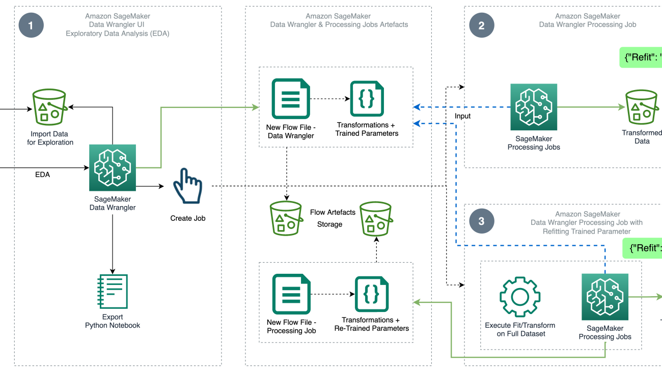
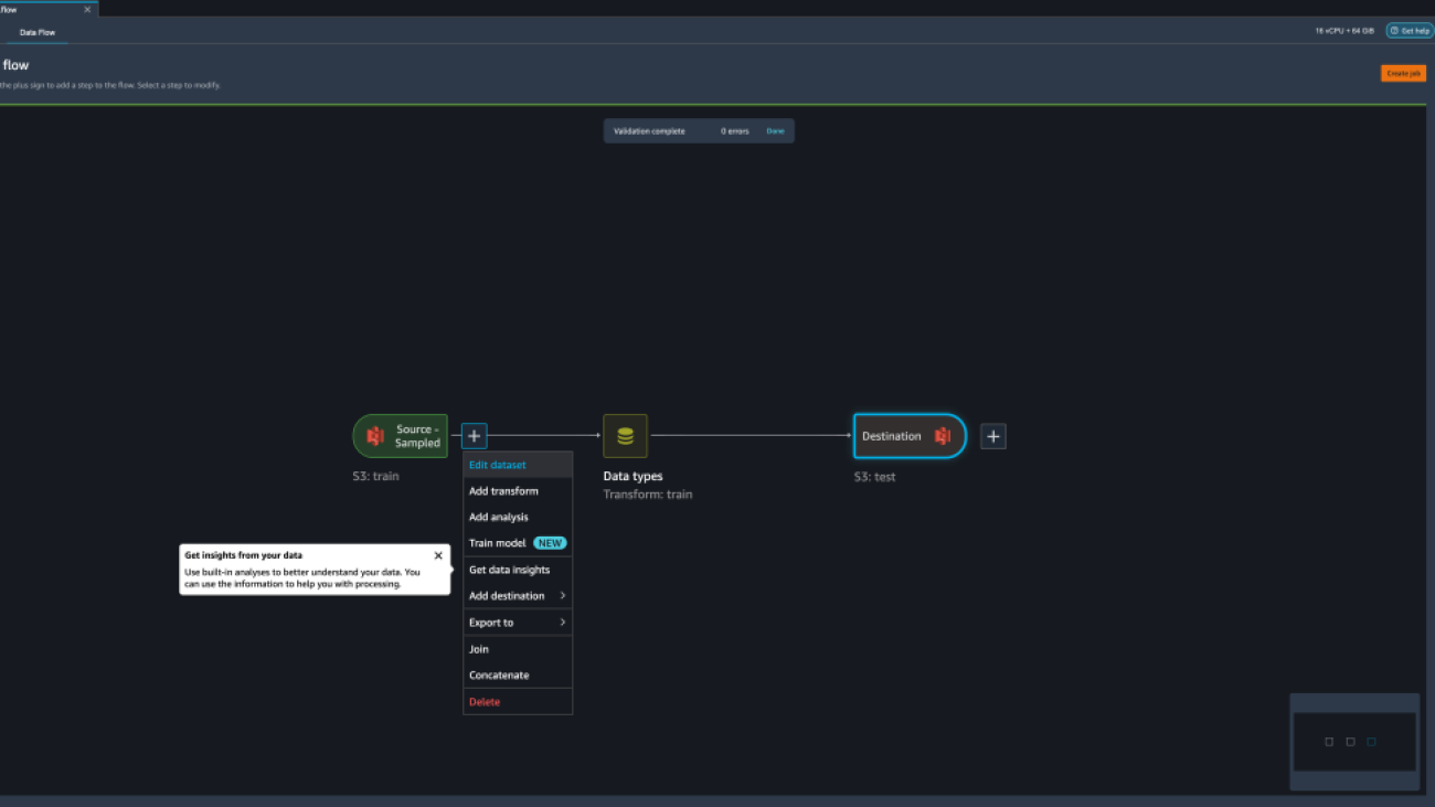
Compare data processing job results

After the Data Wrangler processing jobs are complete, you must create two new Data Wrangler flows with the output generated by the data processing jobs stored in the configured Amazon S3 destination.

You can refer to the configured location in the Amazon S3 destination folder to review the data processing jobs’ outputs.

To inspect the processing job results, create two new Data Wrangler flows using the Data Quality and Insights Report to compare the transformation results.

1. Create a new flow in Amazon SageMaker Data Wrangler.
2. Import the data processing job without refit enabled output file from Amazon S3.
3. Add a new analysis.
4. For Analysis type, choose Data Quality and Insights Report.
5. Choose Create.

Repeat the above steps and create new data wrangler flow to analyze the data processing job output with refit enabled.

Now let’s look at the outputs of processing jobs for the feature property_type using the Data Quality and Insights Reports. Scroll to the feature details on the Data and Insights Reports listing feature_type.

The refit trained parameter processing job has refitted the trained parameters on the entire dataset and encoded the new value APARTMENT with seven distinct values on the full dataset.

The normal processing job applied the sample dataset trained parameters, which have only six distinct values for the property_type feature. For data with feature_type APARTMENT, the invalid handling strategy Skip is applied and the data processing job doesn’t learn this new category. The one-hot encoding has skipped this new category present on the new data, and the encoding skips the category APARTMENT.

Let’s now focus on another feature, city. The refit trained parameter processing job has relearned all the values available for the city feature, considering the new data.

As shown in the Feature Summary section of the report, the new encoded feature column e_city has 100% valid parameters by using the refit trained parameter feature.

In contrast, the normal processing job has 82.4% of missing values in the new encoded feature column e_city. This phenomenon is because only the sample set of learned trained parameters are applied on the full dataset and no refitting is applied by the data processing job.

The following histograms depict the ordinal encoded feature e_city. The first histogram is of the feature transformed with the refit option.

The next histogram is of the feature transformed without the refit option. The orange column shows missing values (NaN) in the Data Quality and Insights Report. The new values that aren’t learned from the sample dataset are replaced as Not a Number (NaN) as configured in the Data Wrangler UI’s invalid handling strategy.

The data processing job with the refit trained parameter relearned the property_type and city features considering the new values from the entire dataset. Without the refit trained parameter, the data processing job only uses the sampled dataset’s pre-learned trained parameters. It then applies them to the new data, but the new values aren’t considered for encoding. This will have implications on the model accuracy.

Clean up

When you’re not using Data Wrangler, it’s important to shut down the instance on which it runs to avoid incurring additional fees.

To avoid losing work, save your data flow before shutting Data Wrangler down.

1. To save your data flow in Amazon SageMaker Studio, choose File, then choose Save Data Wrangler Flow. Data Wrangler automatically saves your data flow every 60 seconds.
2. To shut down the Data Wrangler instance, in Studio, choose Running Instances and Kernels.
3. Under RUNNING APPS, choose the shutdown icon next to the sagemaker-data-wrangler-1.0 app.

4. Choose Shut down all to confirm.

Data Wrangler runs on an ml.m5.4xlarge instance. This instance disappears from RUNNING INSTANCES when you shut down the Data Wrangler app.

After you shut down the Data Wrangler app, it has to restart the next time you open a Data Wrangler flow file. This can take a few minutes.

Conclusion

In this post, we provided an overview of the refit trained parameter feature in Data Wrangler. With this new feature, you can store the trained parameters in the Data Wrangler flow, and the data processing jobs use the trained parameters to apply the learned transformations on large datasets or reinforcement datasets. You can apply this option to vectorizing text features, numerical data, and handling outliers.

Preserving trained parameters throughout the data processing of the ML lifecycle simplifies and reduces the data processing steps, supports robust feature engineering, and supports model training and reinforcement training on new data.

We encourage you to try out this new feature for your data processing requirements.

About the authors

Hariharan Suresh is a Senior Solutions Architect at AWS. He is passionate about databases, machine learning, and designing innovative solutions. Prior to joining AWS, Hariharan was a product architect, core banking implementation specialist, and developer, and worked with BFSI organizations for over 11 years. Outside of technology, he enjoys paragliding and cycling.

Santosh Kulkarni is an Enterprise Solutions Architect at Amazon Web Services who works with sports customers in Australia. He is passionate about building large-scale distributed applications to solve business problems using his knowledge in AI/ML, big data, and software development.

Vishaal Kapoor is a Senior Applied Scientist with AWS AI. He is passionate about helping customers understand their data in Data Wrangler. In his spare time, he mountain bikes, snowboards, and spends time with his family.

Aniketh Manjunath is a Software Development Engineer at Amazon SageMaker. He helps support Amazon SageMaker Data Wrangler and is passionate about distributed machine learning systems. Outside of work, he enjoys hiking, watching movies, and playing cricket.

Read More

Today, we are launching Amazon SageMaker inference on AWS Graviton to enable you to take advantage of the price, performance, and efficiency benefits that come from Graviton chips.

Graviton-based instances are available for model inference in SageMaker. This post helps you migrate and deploy a machine learning (ML) inference workload from x86 to Graviton-based instances in SageMaker. We provide a step-by-step guide to deploy your SageMaker trained model to Graviton-based instances, cover best practices when working with Graviton, discuss the price-performance benefits, and demo how to deploy a TensorFlow model on a SageMaker Graviton instance.

Brief overview of Graviton

AWS Graviton is a family of processors designed by AWS that provide the best price-performance and are more energy efficient than their x86 counterparts. AWS Graviton 3 processors are the latest in the Graviton processor family and are optimized for ML workloads, including support for bfloat16, and twice the Single Instruction Multiple Data (SIMD) bandwidth. When these two features are combined, Graviton 3 can deliver up to three times better performance vs. Graviton 2 instances. Graviton 3 also uses up to 60% less energy for the same performance as comparable Amazon Elastic Compute Cloud (Amazon EC2) instances. This is a great feature if you want to reduce your carbon footprint and achieve your sustainability goals.

Solution overview

To deploy your models to Graviton instances, you either use AWS Deep Learning Containers or bring your own containers compatible with Arm v8.2 architecture.

The migration (or new deployment) of your models from x86 powered instances to Graviton instances is simple because AWS provides containers to host models with PyTorch, TensorFlow, Scikit-learn, and XGBoost, and the models are architecture agnostic. Nevertheless, if you’re willing to bring your own libraries, you can also do so, just ensure that your container is built with an environment that supports Arm64 architecture. For more information, see Building your own algorithm container.

You need to complete three steps to deploy your model:

1. Create a SageMaker model: This will contain, among other parameters, the information about the model file location, the container that will be used for the deployment, and the location of the inference script. (If you have an existing model already deployed in an x86 based inference instance, you can skip this step.)
2. Create an endpoint configuration: This will contain information about the type of instance you want for the endpoint (for example, ml.c7g.xlarge for Graviton3), the name of the model you created in the step 1, and the number of instances per endpoint.
3. Launch the endpoint with the endpoint configuration created in the step 2.

Prerequisites

Before starting, consider the following prerequisites:

1. Complete the prerequisites as listed in Prerequisites.
2. Your model should be either a PyTorch, TensorFlow, XGBoost, or Scikit-learn based model. The following table summarizes the versions currently supported as of this writing. For the latest updates, refer to SageMaker Framework Containers (SM support only).
   

   .	Python	TensorFlow	PyTorch	Scikit-learn	XGBoost
   Versions supported	3.8	2.9.1	1.12.1	1.0-1	1.3-1 to 1.5-1

3. The inference script is stored in Amazon Simple Storage Service (Amazon S3).

In the following sections, we walk you through the deployment steps.

Create a SageMaker model

If you have an existing model already deployed in an x86-based inference instance, you can skip this step. Otherwise, complete the following steps to create a SageMaker model:

1. Locate the model that you stored in an S3 bucket. Copy the URI.
   You use the model URI later in the MODEL_S3_LOCATION.
2. Identify the framework version and Python version that was used during model training.
   You need to select a container from the list of available AWS Deep Learning Containers per your framework and Python version. For more information, refer to Introducing multi-architecture container images for Amazon ECR.
3. Locate the inference Python script URI in the S3 bucket (the common file name is inference.py).
   The inference script URI is needed in the INFERENCE_SCRIPT_S3_LOCATION.
4. With these variables, you can then call the SageMaker API with the following command:

   client = boto3.client("sagemaker")
   
   client.create_model(
       ModelName="Your model name",
       PrimaryContainer={
           "Image": <AWS_DEEP_LEARNING_CONTAINER_URI>,
           "ModelDataUrl": <MODEL_S3_LOCATION>,
           "Environment": {
           "SAGEMAKER_PROGRAM": "inference.py",
           "SAGEMAKER_SUBMIT_DIRECTORY": <INFERENCE_SCRIPT_S3_LOCATION>,
           "SAGEMAKER_CONTAINER_LOG_LEVEL": "20",
           "SAGEMAKER_REGION": <REGION>
           }
       },
       ExecutionRoleArn= <ARN for AmazonSageMaker-ExecutionRole>
   )

You can also create multi-architecture images, and use the same image but with different tags. You can indicate on which architecture your instance will be deployed. For more information, refer to Introducing multi-architecture container images for Amazon ECR.

Create an endpoint config

After you create the model, you have to create an endpoint configuration by running the following command (note the type of instance we’re using):

client.create_endpoint_config(
    EndpointConfigName= <Your endpoint config name>,
    ProductionVariants=[
        {
         "VariantName": "v0",
         "ModelName": "Your model name",
         "InitialInstanceCount": 1,
         "InstanceType": "ml.c7g.xlarge",
        },
    ]
)

The following screenshot shows the endpoint configuration details on the SageMaker console.

Launch the endpoint

With the endpoint config created in the previous step, you can deploy the endpoint:

client.create_endpoint(
    EndpointName = "<Your endpoint name>",
    EndpointConfigName = "<Your endpoint config name>"
    )

Wait until your model endpoint is deployed. Predictions can be requested in the same way you request predictions for your endpoints deployed in x86-based instances.

The following screenshot shows your endpoint on the SageMaker console.

What is supported

SageMaker provides performance-optimized Graviton deep containers for TensorFlow and PyTorch frameworks. These containers support computer vision, natural language processing, recommendations, and generic deep and wide model-based inference use cases. In addition to deep learning containers, SageMaker also provides containers for classical ML frameworks such as XGBoost and Scikit-learn. The containers are binary compatible across c6g/m6g and c7g instances, therefore migrating the inference application from one generation to another is seamless.

C6g/m6g supports fp16 (half-precision float) and for compatible models provides equivalent or better performance compared to c5 instances. C7g substantially increases the ML performance by doubling the SIMD width and supporting bfloat-16 (bf16), which is the most cost-efficient platform for running your models.

Both c6g/m6g and c7g provide good performance for classical ML (for example, XGBoost) compared to other CPU instances in SageMaker. Bfloat-16 support on c7g allows efficient deployment of bf16 trained or AMP (Automatic Mixed Precision) trained models. The Arm Compute Library (ACL) backend on Graviton provides bfloat-16 kernels that can accelerate even the fp32 operators via fast math mode, without the model quantization.

Recommended best practices

On Graviton instances, every vCPU is a physical core. There is no contention for the common CPU resources (unlike SMT), and the workload performance scaling is linear with every vCPU addition. Therefore, it’s recommended to use batch inference whenever the use case allows. This will enable efficient use of the vCPUs by parallel processing the batch on each physical core. If the batch inference isn’t possible, the optimal instance size for a given payload is required to ensure OS thread scheduling overhead doesn’t outweigh the compute power that comes with the additional vCPUs.

TensorFlow comes with Eigen kernels by default, and it’s recommended to switch to OneDNN with ACL to get the most optimized inference backend. The OneDNN backend and the bfloat-16 fast math mode can be enabled while launching the container service:

docker run -p 8501:8501 --name tfserving_resnet 
--mount type=bind,source=/tmp/resnet,target=/models/resnet 
-e MODEL_NAME=resnet -e TF_ENABLE_ONEDNN_OPTS=1 
-e DNNL_DEFAULT_FPMATH_MODE=BF16 -e -t tfs:mkl_aarch64

The preceding serving command hosts a standard resnet50 model with two important configurations:

-e TF_ENABLE_ONEDNN_OPTS=1
-e DNNL_DEFAULT_FPMATH_MODE=BF16

These can be passed to the inference container in the following way:

client.create_model(
    ModelName="Your model name",
    PrimaryContainer={
    "Image": <AWS_DEEP_LEARNING_CONTAINER_URI>,
    "ModelDataUrl": <MODEL_S3_LOCATION>,
    "Environment": {
        "SAGEMAKER_PROGRAM": "inference.py",
        "SAGEMAKER_SUBMIT_DIRECTORY": "<INFERENCE_SCRIPT_S3_LOCATION>",
        "SAGEMAKER_CONTAINER_LOG_LEVEL": "20",
        "SAGEMAKER_REGION": <REGION>,
        "TF_ENABLE_ONEDNN_OPTS": "1",
        "DNNL_DEFAULT_FPMATH_MODE": "BF16"
         }
     },
     ExecutionRoleArn='ARN for AmazonSageMaker-ExecutionRole'
)

Deployment example

In this post, we show you how to deploy a TensorFlow model, trained in SageMaker, on a Graviton-powered SageMaker inference instance.

You can run the code sample either in a SageMaker notebook instance, an Amazon SageMaker Studio notebook, or a Jupyter notebook in local mode. You need to retrieve the SageMaker execution role if you use a Jupyter notebook in local mode.

The following example considers the CIFAR-10 dataset. You can follow the notebook example from the SageMaker examples GitHub repo to reproduce the model that is used in this post. We use the trained model and the cifar10_keras_main.py Python script for inference.

The model is stored in an S3 bucket: s3://aws-ml-blog/artifacts/run-ml-inference-on-graviton-based-instances-with-amazon-sagemaker/model.tar.gz

The cifar10_keras_main.py script, which can be used for the inference, is stored at:s3://aws-ml-blog/artifacts/run-ml-inference-on-graviton-based-instances-with-amazon-sagemaker/script/cifar10_keras_main.py

We use the us-east-1 Region and deploy the model on an ml.c7g.xlarge Graviton-based instance. Based on this, the URI of our AWS Deep Learning Container is 763104351884.dkr.ecr.us-east-1.amazonaws.com/tensorflow-inference-graviton:2.9.1-cpu-py38-ubuntu20.04-sagemaker

1. Set up with the following code:

   import sagemaker
   import boto3
   import datetime
   import json
   import gzip
   import os
   
   sagemaker_session = sagemaker.Session()
   bucket = sagemaker_session.default_bucket()
   role = sagemaker.get_execution_role()
   region = sagemaker_session.boto_region_name

2. Download the dataset for endpoint testing:

   from keras.datasets import cifar10
   (x_train, y_train), (x_test, y_test) = cifar10.load_data()

3. Create the model and endpoint config, and deploy the endpoint:

   timestamp = "{:%Y-%m-%d-%H-%M-%S}".format(datetime.datetime.now())
   
   client = boto3.client("sagemaker")
   
   MODEL_NAME = f"graviton-model-{timestamp}"
   ENDPOINT_NAME = f"graviton-endpoint-{timestamp}"
   ENDPOINT_CONFIG_NAME = f"graviton-endpoint-config-{timestamp}"
   
   # create sagemaker model
   create_model_response = client.create_model(
       ModelName=MODEL_NAME,
       PrimaryContainer={
       "Image":  "763104351884.dkr.ecr.us-east-1.amazonaws.com/tensorflow-inference-graviton:2.9.1-cpu-py38-ubuntu20.04-sagemaker ",
       "ModelDataUrl":  "s3://aws-ml-blog/artifacts/run-ml-inference-on-graviton-based-instances-with-amazon-sagemaker/model.tar.gz",
       "Environment": {
           "SAGEMAKER_CONTAINER_LOG_LEVEL": "20",
           "SAGEMAKER_REGION": region
           }
       },
       ExecutionRoleArn=role
   )
   print ("create_model API response", create_model_response)

4. Optionally, you can add your inference script to Environment in create_model if you didn’t originally add it as an artifact to your SageMaker model during training:

   "SAGEMAKER_PROGRAM": "inference.py",
   "SAGEMAKER_SUBMIT_DIRECTORY": <INFERENCE_SCRIPT_S3_LOCATION>,
   		
   # create sagemaker endpoint config
   create_endpoint_config_response = client.create_endpoint_config(
       EndpointConfigName=ENDPOINT_CONFIG_NAME,
       ProductionVariants=[
           {
            "VariantName": "v0",
            "ModelName": MODEL_NAME,
            "InitialInstanceCount": 1,
            "InstanceType": "ml.c7g.xlarge" 
           },
       ]
   )
   print ("ncreate_endpoint_config API response", create_endpoint_config_response)
   
   # create sagemaker endpoint
   create_endpoint_response = client.create_endpoint(
       EndpointName = ENDPOINT_NAME,
       EndpointConfigName = ENDPOINT_CONFIG_NAME,
   )
   print ("ncreate_endpoint API response", create_endpoint_response)   
   

   You have to wait a couple of minutes for the deployment to take place.

5. Verify the endpoint status with the following code:

   describe_response = client.describe_endpoint(EndpointName=ENDPOINT_NAME)
   print(describe_response["EndpointStatus"]

   You can also check the AWS Management Console to see when your model is deployed.

6. Set up the runtime environment to invoke the endpoints:

   runtime = boto3.Session().client(service_name="runtime.sagemaker")

   Now we prepare the payload to invoke the endpoint. We use the same type of images used for the training of the model. These were downloaded in previous steps.

7. Cast the payload to tensors and set the correct format that the model is expecting. For this example, we only request one prediction.

   input_image = x_test[0].reshape(1,32,32,3)

   We get the model output as an array.

8. We can turn this output into probabilities if we apply a softmax to it:

   CONTENT_TYPE = 'application/json'
   ACCEPT = 'application/json'
   PAYLOAD = json.dumps(input_image.tolist())
   
   response = runtime.invoke_endpoint(
       EndpointName=ENDPOINT_NAME, 
       ContentType=CONTENT_TYPE,
       Accept=ACCEPT,
       Body=PAYLOAD
   )
       
   print(response['Body'].read().decode())

Clean up resources

The services involved in this solution incur costs. When you’re done using this solution, clean up the following resources:

client.delete_endpoint(EndpointName=ENDPOINT_NAME)
client.delete_endpoint_config(EndpointConfigName=ENDPOINT_CONFIG_NAME)
client.delete_model(ModelName=MODEL_NAME)

Price-performance comparison

Graviton-based instances offer the lowest price and the best price-performance when compared to x86-based instances. Similar to EC2 instances, the SageMaker inference endpoints with ml.c6g instances (Graviton 2) offer a 20% lower price compared to ml.c5, and the Graviton 3 ml.c7g instances are 15% cheaper than ml.c6 instances. For more information, refer to Amazon SageMaker Pricing.

Conclusion

In this post, we showcased the newly launched SageMaker capability to deploy models in Graviton-powered inference instances. We gave you guidance on best practices and briefly discussed the price-performance benefits of the new type of inference instances.

To learn more about Graviton, refer to AWS Graviton Processor. You can get started with AWS Graviton-based EC2 instances on the Amazon EC2 console and by referring to AWS Graviton Technical Guide. You can deploy a Sagemaker model endpoint for inference on Graviton with the sample code in this blog post.

About the authors

Victor Jaramillo, PhD, is a Senior Machine Learning Engineer in AWS Professional Services. Prior to AWS, he was a university professor and research scientist in predictive maintenance. In his free time, he enjoys riding his motorcycle and DIY motorcycle mechanics.

Zmnako Awrahman, PhD, is a Practice Manager, ML SME, and Machine Learning Technical Field Community (TFC) member at Amazon Web Services. He helps customers leverage the power of the cloud to extract value from their data with data analytics and machine learning.

Sunita Nadampalli is a Software Development Manager at AWS. She leads Graviton software performance optimizations for machine leaning, HPC, and multimedia workloads. She is passionate about open-source development and delivering cost-effective software solutions with Arm SoCs.

Johna Liu is a Software Development Engineer in the Amazon SageMaker team. Her current work focuses on helping developers efficiently host machine learning models and improve inference performance. She is passionate about spatial data analysis and using AI to solve societal problems.

Alan Tan is a Senior Product Manager with SageMaker, leading efforts on large model inference. He’s passionate about applying machine learning to the area of analytics. Outside of work, he enjoys the outdoors.

Read More