Posts in category: Amazon AWS

Amazon SageMaker is a fully-managed service that provides every developer and data scientist with the ability to quickly build, train, and deploy machine learning (ML) models at scale. ML is realized in inference. SageMaker offers four Inference options:

1. Real-Time Inference
2. Serverless Inference
3. Asynchronous Inference
4. Batch Transform

These four options can be broadly classified into Online and Batch inference options. In Online Inference, requests are expected to be processed as they arrive, and the consuming application expects a response after each request is processed. This can either happen synchronously (real-time Inference, serverless) or asynchronously (asynchronous inference). In a synchronous pattern, the consuming application is blocked and can’t proceed until it receives a response. These workloads tend to be real-time applications, such as online credit card fraud detection, where responses are expected in the order of milliseconds to seconds and request payloads are small (a few MB). In the asynchronous pattern, the application experience isn’t blocked (for example, submitting an insurance claim via a mobile app), and usually requires larger payload sizes and/or longer processing times. In Offline inference, an aggregation (batch) of inference requests are processed together, and responses are provided only after the entire batch has been processed. Usually, these workloads aren’t latency sensitive, involve large volumes (multiple GBs) of data, and are scheduled at a regular cadence (for example, run object detection on security camera footage at the end of the day or process payroll data at the end of the month).

At the bare bones, SageMaker Real-Time Inference consists of a model(s), the framework/container with which you’re working, and the infrastructure/instances that are backing your deployed endpoint. In this post, we’ll explore how you can create and invoke a Single Model Endpoint.

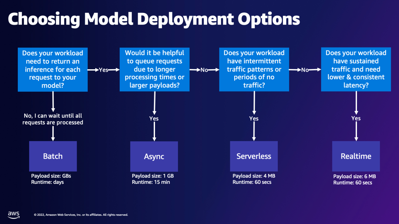
Choosing model deployment option

Choosing the right inference type can be difficult, and the following simple guide can help you. It’s not a strict flow chart, so if you find that another option works better for you, then feel free to use those. In particular, Real-Time Inference is a great option for hosting your models when you have low and consistent latency (in the order of milliseconds or seconds) and throughput sensitive workloads. You can control the instance type and count behind your endpoint while also configuring AutoScaling policy to handle traffic. There are two other SageMaker Inference options that you can also use to create an endpoint. Asynchronous Inference is when you have large payload sizes and near real-time latency bandwidth. This is a good option, especially for NLP and Computer Vision models that have longer preprocessing times. Serverless Inference is a great option when you have intermittent traffic and don’t want to manage infrastructure scaling. The recipe for creating an endpoint remains the same regardless of the Inference type that you choose. In this post, we’ll focus on creating a real-time instance-based endpoint, but you can easily adapt it to either of the other Inference Options based on your use-case. Lastly, Batch inference takes place offline, so you can provide a set of data that you want to get inference from and we’ll run it. This is similarly instance-based, so you can select the optimal instance for your workload. As there is no endpoint up and running, you only pay for the duration of the job. It is good for processing gigabytes of data and the job duration can be days. There are built-in features to make working with structured data easier and optimizations to automatically distribute structured data. Some example use cases are propensity modeling, predictive maintenance, and churn prediction. All of these can take place offline in bulk because it doesn’t have to react to a specific event.

Hosting a model on SageMaker Endpoints

At the crux, SageMaker Real-Time Endpoints consists of a model and the infrastructure with which you choose to back the Endpoint. SageMaker uses containers to host models, which means that you need a container that properly sets up the environment for the framework that you use for each model that you provide. For example, if you’re working with a Sklearn model, you must pass in your model scripts/data within a container that properly sets up Sklearn. Luckily, SageMaker provides managed images for popular frameworks, such as TensorFlow, PyTorch, Sklearn, and HuggingFace. You can retrieve and utilize these images using the high-level SageMaker Python SDK and inject your model scripts and data into these containers. In the case that SageMaker doesn’t have a supported container, you can also Build Your Own Container and push your own custom image, installing the dependencies that are necessary for your model.

SageMaker supports both trained and pre-trained models. In the previous paragraph when we’re talking about model scripts/data, we’re referencing this matter. You can either mount a script on your container, or if you have a pre-trained model artifact (for example, `model.joblib` for SKLearn), then you can provide this along with your image to SageMaker. To understand SageMaker Inference, there are three main entities that you’ll create in the process of Endpoint creation:

1. SageMaker Model Entity – Here you can pass in your trained model data/model script and your image that you’re working with, whether it’s owned by AWS or built by you.
2. Endpoint configuration creation – Here you define your infrastructure, meaning that you select the instance type, count, etc.
3. Endpoint creation – This is the REST Endpoint that hosts your model that you’re invoking to get a response. Let’s look at how you can utilize a managed SageMaker Image and your own custom-built image to deploy an endpoint.

Real-time endpoint requirements

1. Before creating an Endpoint, you must understand what type of Model you want to host. If it’s a Framework model, such as TensorFlow, PyTorch, or MXNet, then you can utilize one of the prebuilt Framework images.
   If it’s a custom model, or you would like full flexibility in creating the container that SageMaker will run for inference, then you can build your own container.

SageMaker Endpoints are made up of a SageMaker Model and Endpoint Configuration.
If you’re using Boto3, then you would create both objects. Otherwise, if you’re utilizing the SageMaker Python SDK, then the Endpoint Configuration is created on your behalf when you use the .deploy(..) function.

SageMaker entities:

• SageMaker Model:
  • Contains the details of the inference image, location of the model artifacts in Amazon Simple Storage Service (Amazon S3), network configuration, and AWS Identity and Access Management (IAM) role to be used by the Endpoint.
    • SageMaker requires your model artifacts to be compressed in a .tar.gz file. SageMaker automatically extracts this .tar.gz file into the /opt/ml/model/ directory in your container. If you’re utilizing one of the framework containers, such as TensorFlow, PyTorch, or MXNet, then the container expects your TAR structure to be as follows:
      • TensorFlow
        

        model.tar.gz/
        |--[model_version_number]/
        |--variables
        |--saved_model.pb
        code/
        |--inference.py
        |--requirements.txt

      • PyTorch
        

        model.tar.gz/
        |- model.pth
        |- code/
        |- inference.py
        |- requirements.txt # only for versions 1.3.1 and higher

      • MXNet
        

        model.tar.gz/
        |- model-symbol.json
        |- model-shapes.json
        |- model-0000.params
        |- code/
            |- inference.py
            |- requirements.txt # only for versions 1.6.0 and higher

      • Sklearn
        

        model.tar.gz/
        |- model.joblib
        | code/ 
        |- inference.py

    • When utilizing a Framework image, we can provide a custom entry-point script, where we can implement our own pre and post processing. In our case, the inference script is packaged in the model.tar.gz under the /code directory.

• • Endpoint Configuration
    • Contains the infrastructure information required to deploy the SageMaker Model to the Endpoint.
    • For example, the SageMaker Model we created is specified here as well as the Instance Type and Initial Instance count.

Frameworks and BYOC

• • Retrieving SageMaker images
    • This portion isn’t always necessary and abstracted out by the SageMaker Python SDK via estimators. However, if you would like to be able to retrieve a SageMaker managed image to extend on it, then you can get the images that are available via the SDK. The following is an example of retreiving a TF 2.2 image for inference.

      import sagemaker
      tf_image = sagemaker.image_uris.retreive(framework="tensorflow", region="us-east-1",
      image_scope = "inference", version = "2.2", instance_type = "ml.c5.xlarge)
      print(tf_image)

  • Frameworks
    • In the case that you want to deploy a Framework Model, such as TensorFlow, PyTorch, or MXNet, then all you need is the model artifacts.
    • See the documentation for deploying models directly from model artifacts for TensorFlow, PyTorch, or MXNet.

• • Choosing between 1P and BYOC
    • The SageMaker SDK also abstracts handling the image out, as you saw in the previous Frameworks section. It has ready-made estimators for Sklearn, TensorFlow, and PyTorch that automatically select the image for you based off of the version that you’ve selected. Then you can pass in a training/inference script through Script Mode into these estimators.

      from sagemaker.pytorch import PyTorch #PyTorch Estimator within SageMaker SDK
      estimator_parameters = {"entry_point": "train_deploy_pytorch_without_dependencies.py",
      "source_dir": "pytorch_script","instance_type": train_instance_type,
      "instance_count": 1,"hyperparameters": hyperparameters,
      "role": role,"base_job_name": "pytorch-model","framework_version": "1.5",
      "py_version": "py3",}
      
      ## Model Training
      estimator = PyTorch(**estimator_parameters)estimator.fit(inputs)
      
      ## Deploy Trained model
      pytorch_predictor = estimator.deploy(initial_instance_count=1, instance_type="ml.m5.xlarge", endpoint_name=pytorch_endpoint_name)

    • Not all packages and images are supported by SageMaker, and in this case you must bring your own container (BYOC). This means building a Dockerfile that will setup the proper environment for your model serving. An example of this is the Spacy NLP module, and there are no managed SageMaker containers for this framework. Therefore, you must provide a Dockerfile that installs Spacy. Within the container you also mount your model inference scripts. Let’s quickly discuss the components that you provide in a Bring Your Own Container format, as these stay consistent for most examples.
      • “nginx.conf“ is the configuration file for the nginx front-end. You won’t have to edit this file, unless you would like to tune these portions.
      • “predictor.py“ is the program that actually implements the Flask web server and model code for your application. You can have further Python files or functions in your container that you can call in this file.
      • “serve“ is the program started when the container is started for hosting. It simply launches the gunicorn server, which runs multiple instances of the Flask app defined in predictor.py. Like nginx.conf, you don’t have to edit this file unless there’s further tuning that you would like to perform.
      • “train“ is the program that is invoked when the container is run for training. You’ll modify this program to implement your training algorithm. If you’re bringing a pre-trained model or framework like Spacy, then you don’t need this file.
      • “wsgi.py“ is a small wrapper used to invoke the Flask app. You should be able to take this file as-is, unless you’ve changed the name of your predictor.py file. In that case, make sure that maps properly here.

• • Custom inference script
    • SageMaker Framework containers give you the flexibility to handle pre/post processing of the request and model loading using a custom entry point script/inference.py.
    • See the documentation for creating a custom inference.py script for TensorFlow, PyTorch and MXNet.
  • Custom container
    • Custom containers allow you full autonomy in using your own inference code to host your model. Your container is required to comply with certain API contracts. For example, it must respond to /invocations and /ping on port 8080. This Scikit Bring Your Own Container example showcases a common hosting pattern of NGINXGunicornFlask.

Different ways that you can interact with SageMaker Endpoints

There are many options for using SageMaker programmatically so that you can call your deployed models to get inference. The AWS Command Line Interface (AWS CLI), REST APIs, AWS CloudFormation, AWS Cloud Development Kit (AWS CDK), and AWS SDKs are common tools offered by AWS and widely supported by other AWS services. For SageMaker, we also have a SageMaker Python SDK. Now, let’s compare the different options to create, invoke, and manage SageMaker Endpoints.

In addition to SageMaker CLI, there are two ways programmatically that you can interact with Endpoints in SageMaker through the SDKs. Let’s look at some differences between SageMaker Python SDK and Boto3 Python SDK:

1. High-level SageMaker “Python” SDK – This SDK is an open-source library that provides higher level abstraction specifically meant for calling SageMaker APIs programmatically using Python. The Good part of this SDK is that it’s very easy to call sagemaker APIs, lots of heavy lifting is done already like calling the APIs synchronously/async mode (helps to avoid polling), simpler request/response schema, much less code, and much simpler code. SageMaker Python SDK provides several high-level abstractions for working with SageMaker. The package is meant to simplify different ML processes on SageMaker.
2. Low-level AWS SDK (Boto3 SDK) – This SDK works at the lower level by allowing the user to choose from the supported programming languages and call any AWS services programmatically. This isn’t just specific to SageMaker but can be used in general for all AWS services. The low-level AWS SDKs are available in various programming languages, such as .NET, Python, Java, Node.js, etc. One of the popular SDKs used is boto3 python SDK, which is popular in the data scientist community for ML. The good part of this SDK is that it’s very lightweight and available by default installed on AWS Lambda Runtime. Furthermore, you can use this SDK to interact with any AWS service outside of SageMaker.

Both of these SDKs can be utilized for the same tasks, but in some cases it’s more intuitive to use one more than the other. SageMaker Python SDK is recommended for easy testing while AWS SDK/Boto3 is recommended for production use cases for better control on performance. For example, SageMaker as a service provides pre-built and maintained images for popular frameworks, such as Sklearn, PyTorch, and TensorFlow. It can be particularly useful to use SageMaker SDK to retrieve deep learning images, train models using Estimators, and easily deploy the model using a simple API call. An example to showcase this in action can be found here.

On the other hand, sometimes you have pre-trained models or different frameworks that you may be using. This requires a greater deal of customization and the SageMaker SDK doesn’t always offer that. We have three important steps and corresponding boto3 API calls that we need to execute to deploy an endpoint: Model Creation, Endpoint Configuration Creation, and Endpoint Creation. The first two entities were abstracted out with the SageMaker SDK with our supported frameworks, but we see those details with the Boto3 SDK. An extensive example to showcase the steps involved in using a Boto3 SDK to create and manage an endpoint can be found here.

Considerations of SageMaker hosting

SageMaker Real-Time Inference has two main optimizations that you can consider: 1/ Performance optimization, and 2/ Cost optimization. Let’s first look at performance optimization, as when we’re dealing with latency sensitive workloads, every millisecond is crucial. There are different knobs that you can tune to optimize your latency and throughput. At the instance level, you can use Inference Recommender, our built-in load testing tool, to help you select the right instance type and count for your workload. Utilizing the proper combination of compute will help you with both performance and cost. You can also tune at the container and framework level.
Questions to ask yourself include:

1. What framework are you using?
2. Are there any environment variables that you can tune within your container?

An example of this is maximizing TensorFlow performance with SageMaker containers. Another example of container level optimizations is utilizing gRPC rather than REST behind your endpoint. Lastly, you can also optimize at the script level. Is your inference code taking extra time at certain blocks? Timing each and every line of your script will help you capture any bottlenecks within your code.

There are three ways to look at improving the utilization of your Real Time endpoint:

1. Multi-model Endpoints (MME)
   • You can host thousands of models behind a single endpoint. This is perfect for use cases where you don’t need a dedicated endpoint for each one of your models. MME works best when the models are similarly sized and latency and belong to the same ML framework. These can be typically used when you don’t need to call the same model at all times. You can dynamically load the respective model onto the SageMaker Endpoint to serve your request. An example that showcases MME in action can be found here. If you want to learn more about the different caveats and best practices for hosting models on MME, then refer to the post here.
2. Multi-Container Endpoints (MCE)
   • Instead of utilizing multiple endpoints to host multiple containers, you can look at hosting up to 15 containers on a single endpoint. Each one of these containers can be invoked directly. Therefore, you can look at hosting disparate models of different frameworks all on a single endpoint. This option is best when containers exhibit similar usage and performance characteristics. An example that showcases MCE can be found here. If you want to learn more about the different caveats and best practices for hosting models on MCE, then refer to the post here.
3. Serial Inference Pipeline (SIP)
   • If you have a pipeline of steps in your inference logic, then you might utilize Serial Inference Pipeline (SIP). SIP lets you chain 2-15 containers together behind a single endpoint. SIP works well when you have preprocessing and post-processing steps. If you want to learn more about the design patterns for serial inference pipelines, then refer to the post here.

The second main optimization to keep in mind is cost. Real-Time Inference is one of three options within creating SageMaker Endpoints. SageMaker Endpoints are running at all times unless deleted. Therefore, you must look at improving the utilization of the endpoint which in turn provides a cost benefit.

SageMaker also offers Savings Plans. Savings Plans can reduce your costs by up to 64%. This is a 1 or 3-year term commitment to a consistent amount of usage ($/hour). See this link for more information. And see this link for best to optimize costs for Inference on Amazon SageMaker.

Conclusion

In this post, we showed you some of the best practices to choose between different model hosting options on SageMaker. We discussed the SageMaker Endpoint requirements, and also contrasted Framework and BYOC requirements and functionality. Furthermore, we talked about the different ways that you can leverage Real-Time Endpoints to host your ML models in production. in a cost-effective way, and have high performance.

See the corresponding GitHub repository and try out the examples.

About the authors

Raghu Ramesha is an ML Solutions Architect with the Amazon SageMaker Service team. He focuses on helping customers build, deploy, and migrate ML production workloads to SageMaker at scale. He specializes in machine learning, AI, and computer vision domains, and holds a master’s degree in Computer Science from UT Dallas. In his free time, he enjoys traveling and photography.

Ram Vegiraju is a ML Architect with the SageMaker Service team. He focuses on helping customers build and optimize their AI/ML solutions on Amazon SageMaker. In his spare time, he loves traveling and writing.

Marc Karp is a ML Architect with the SageMaker Service team. He focuses on helping customers design, deploy and manage ML workloads at scale. In his spare time, he enjoys traveling and exploring new places.

Dhawal Patel is a Principal Machine Learning Architect at AWS. He has worked with organizations ranging from large enterprises to mid-sized startups on problems related to distributed computing and artificial intelligence. He focuses on deep learning, including NLP and computer vision domains. He helps customers achieve high-performance model inference on Amazon SageMaker.

Saurabh Trikande is a Senior Product Manager for Amazon SageMaker Inference. He is passionate about working with customers and is motivated by the goal of democratizing machine learning. He focuses on core challenges related to deploying complex ML applications, multi-tenant ML models, cost optimizations, and making deployment of deep learning models more accessible. In his spare time, Saurabh enjoys hiking, learning about innovative technologies, following TechCrunch, and spending time with his family.

Read More

Non-small cell lung cancer (NSCLC) is the most common type of lung cancer, and is composed of tumors with significant molecular heterogeneity resulting from differences in intrinsic oncogenic signaling pathways [1]. Enabling precision medicine, anticipating patient preferences, detecting disease, and improving care quality for NSCLC patients are important topics among healthcare and life sciences (HCLS) communities.

Applying machine learning (ML) to diverse health datasets, known as multimodal machine learning (multimodal ML), is an active area of research and development. Analyzing linked patient-level data from diverse data modalities, such as genomics and medical imaging, promises to accelerate improvements in patient care. However, performing analyses of multiple modalities at scale has been challenging in on-premises or cloud environments due to the distinct infrastructure requirements of each modality. With Amazon SageMaker, you can create purpose-built pipelines and scale them to meet your needs easily, paying only for what you use.

We’re announcing a new solution on lung cancer survival prediction in Amazon SageMaker JumpStart, based on the blog posts Building Scalable Machine Learning Pipelines for Multimodal Health Data on AWS and Training Machine Learning Models on Multimodal Health Data with Amazon SageMaker. JumpStart provides pre-trained, open-source models and pre-built solution templates for a wide range of problem types to help data scientists and ML practitioners get started on training and deploying ML models quickly. This is the first HCLS solution offered by JumpStart.

The solution builds a multimodal ML model for predicting survival outcome of patients diagnosed with NSCLC. The multimodal model is trained on data derived from different modalities or domains, including medical imaging, genomic, and clinical data. Multimodal ML has been adopted in HCLS for personalized treatment, clinical decision support, and drug response prediction. In this post, we demonstrate how you can create a scalable, purpose-built ML pipeline easily with one-click deployment from JumpStart.

What’s in the dataset

Non–small cell lung cancer is the leading cause for cancer death [2]. However, no two cancer diagnoses are alike, because tumors contain significant molecular heterogeneity resulting from differences in intrinsic oncogenic signaling pathways [1]. In addition, different clinical information collected from patients may impact prognosis and treatment options. Therefore, enabling precision medicine, anticipating patient preferences, detecting disease, and improving care quality for NSCLC patients is of utmost importance in the oncology and HCLS communities.

The Non-Small Cell Lung Cancer (NSCLC) Radiogenomic dataset [3] comprises medical imaging, clinical, and genomic data collected from a cohort of early-stage NSCLC patients referred for surgical treatment. It includes Computed Tomography (CT), Positron Emission Tomography (PET)/CT images, semantic annotations of the tumors as observed on the medical images using a controlled vocabulary, segmentation maps of tumors in the CT scans, and quantitative values obtained from the PET/CT scans. The genomic data contains gene mutation and RNA sequencing data from samples of surgically excised tumor tissue. It also consists of clinical data reflective of electronic health records (EHR) such as age, gender, weight, ethnicity, smoking status, Tumor Node Metastasis (TNM) stage, histopathological grade, and survival outcome. Each data modality presents a different view of a patient.

Medical imaging data

Medical imaging biomarkers of cancer promise improvements in patient care through advances in precision medicine. Compared to genomic biomarkers, imaging biomarkers provide the advantages of being non-invasive, and characterizing a heterogeneous tumor in its entirety, as opposed to limited tissue available via biopsy [3]. In this dataset, CT and PET/CT imaging sequences were acquired for patients prior to surgical procedures. Segmentation of tumor regions were annotated by two expert thoracic radiologists. The following image is an example overlay of a tumor segmentation onto a lung CT scan (case R01-093 in the dataset).

Genomic data

Samples of surgically excised tumor tissues were analyzed with RNA sequencing technology. The dataset file that is available from the source was preprocessed using open-source tools, including STAR v.2.3 for alignment and Cufflinks v.2.0.2 for expression calls [4]. The original dataset (GSE103584_R01_NSCLC_RNAseq.txt.gz) can be found on the NCBI website. Although the original data contains more than 22,000 genes, for the purpose of demonstration, we used 21 genes from 10 highly co-expressed gene clusters (metagenes) that were identified, validated in publicly available gene-expression cohorts, and correlated with prognosis [4].

The following table shows the tabular representation of the gene expression data. Each row corresponds to a patient, and the columns represent a subset of genes selected for demonstration. The value denotes the expression level of a gene for a patient. A higher value means the corresponding gene is highly expressed in that specific tumor sample.

Clinical data

Clinical data was collected from medical records. It included demographics, smoking history, survival, recurrence status, histology, histopathological grading, Pathological TNM staging, and survival outcome of patients. The data is stored in CSV format, as shown in the following table.

Solution overview

Working with multimodal healthcare data for ML purposes often requires dedicated data processing pipelines and compute resources to extract relevant biomarkers and features. Collecting, storing, and managing extracted features can be challenging. In this JumpStart solution, we show you how to process each modality in separate notebooks, use Amazon SageMaker Processing for compute intensive 3D image construction, use Amazon SageMaker Feature Store to centrally store extracted features for ML modeling, run SageMaker experiments to enhance ML lineage, implement the SageMaker built-in algorithm to train an ML model without sophisticated coding, and deploy a model for real-time prediction with SageMaker deployment.

The architecture for the solution is illustrated in the following diagram.

The key services involved are as follows:

• Amazon SageMaker JumpStart – JumpStart provides pre-trained, open-source models for a wide range of problem types to help you get started. JumpStart also provides solution templates that set up infrastructure for common use cases, and notebooks for ML with SageMaker. This service is where we launch our solution.
• Amazon Simple Storage Service – Amazon S3 is an object storage service that offers scalability, data availability, security, and performance. Amazon S3 allows you to store data to be used by SageMaker.
• Amazon SageMaker Studio notebooks – You can launch these collaborative notebooks quickly because you don’t need to set up compute instances and file storage beforehand. This is the environment you can build in.
• SageMaker Processing jobs – These jobs enable you to analyze data and evaluate ML models. This managed experience helps you run your data processing workloads, such as feature engineering, data validation, and model interpretation. This service allows you to process the data that is stored in Amazon S3.
• Amazon SageMaker Feature Store – You can create, share, and manage features for ML development. This is where you store processed features to use for training.
• Amazon SageMaker Experiments – You can organize, track, compare, and evaluate ML experiments.
• Built-in XGBoost algorithm (eXtreme gradient boosting) – This is a popular and efficient open-source implementation of the gradient boosting algorithm that is used for training the.
• SageMaker training jobs – You create a managed training job in SageMaker using four attributes: the URL of the S3 bucket you’ve stored the training data, compute resources, the URL of the S3 bucket where you want to store the output of the job, and the Amazon Elastic Container Registry (Amazon ECR) path where the training code is stored.
• SageMaker real-time endpoints – These endpoints are ideal for inference workloads where you have real-time, interactive, low-latency requirements. You deploy the model to SageMaker hosting services and get an endpoint that can be used for inference.

With this JumpStart solution, you can easily spin up the solution in Amazon SageMaker Studio, and follow the post to explore, train, and deploy a lung cancer survival status prediction model for learning purposes.

Prerequisites

To use the Lung Cancer Survival Prediction solution provided by JumpStart, you need to have a Studio domain. A SageMaker project and JumpStart must also be enabled.

If you don’t have a Studio domain, refer to Onboard to Amazon SageMaker Domain Using Quick Setup.

If you have a SageMaker domain, make sure that the project and JumpStart features have been enabled by following these steps:

1. On the SageMaker console, choose the gear icon next to Domain.
2. Choose Next.
3. In the SageMaker Projects and JumpStart section, select Enable Amazon SageMaker project templates and Amazon SageMaker JumpStart for this account and Enable Amazon SageMaker project templates and Amazon SageMaker JumpStart for Studio users.

We have completed the prerequisites needed to use JumpStart.

Deploy the solution and example demo notebook

To start using the Lung Cancer Survival Prediction solution, complete the following steps:

1. Open Studio.
2. Choose Go to SageMaker JumpStart under Jumpstart models, algorithms, and solutions.
   
3. To find the solution within JumpStart, choose Explore All Solutions.
   
4. Search for and choose Lung Cancer Survival Prediction.
   
5. Under Launch Solution, choose Launch.
   Note that you can specify custom execution roles to be used throughout this solution, otherwise execution roles are created for you.
   It should take a few moments for the solution to launch. You can follow along as a number of resources are launched.

   Wait until the endpoint and model statuses show as Complete. You may need to refresh the page.

   

   This solution generates a model, endpoint configuration, endpoint, and five notebooks.

6. To navigate to the first notebook, under Open solution in Studio, choose Open Notebook.
7. To navigate to other notebooks, select the folder icon and open the S3Downloads folder.
8. Open the jumpstart-prod-lcsp_****** folder.

Form here, you can access the following notebooks:

• 0_demo.ipynb – Demonstrates how to send inference requests to a pre-deployed endpoint and receive a model response.
• 1_preprocess_genomic_data.ipynb – Showcases how to read and process genomic data (in tabular format).
• 2_preprocess_clinical_data.ipynb – Demonstrates how to read and process health insurance claims data (in tabular format).
• 3_preprocess_imaging_data.ipynb – Showcases how to read and process medical imagining data in DICOM file format and convert to NIfTI neuroimaging format. Therefore, it takes medical imagining data in volumetric format. Note that in notebooks 1, 2, and 3, we store the output of each processing job in Feature Store.
• 4_train_test_model.ipynb – Demonstrates how to access multimodal features from Feature Store, train an XGBoost model, and predict the survival status of patients diagnosed with non-small cell lung cancer.

After the solution is deployed in Studio, you can start building a lung cancer survival status prediction using multimodal health data. To start, let’s look at the 0_demo.ipynb notebook, which demonstrates how to send inference requests to a pre-deployed endpoint, and get the model response (survived vs. dead).

In this notebook, you can see a preview of the datasets (which we cover in a later section), and the steps needed to make predictions with an endpoint that has already been deployed. A predictor is instantiated to begin making real-time predictions against a SageMaker endpoint. We can use the predictor’s predict function to invoke the endpoint with test data.

The endpoint returns the predicted survival status, which is used to assess model performance, as shown in the following screenshot.

Feature engineering

As described earlier, genomic, clinical, and medical imaging data is available in the NSCLC dataset for us to create a comprehensive view of a patient. To process and compute the features that later help us build a ML model, let’s start with the genomic data pipeline in 1_preprocess_genomic_data.ipynb and step through 2_preprocess_clinical_data.ipynb and 3_preprocess_imaging_data.ipynb for the clinical data pipeline and medical imaging pipeline, respectively.

Genomic

For genomic data, we read the RNA sequence data from the JumpStart solution bucket into the notebook 1_preprocess_genomic_data.ipynb:

file_name = "GSE103584_R01_NSCLC_RNAseq.txt"
input_data_bucket = f"s3://{SOLUTION_BUCKET}-{REGION}/{SOLUTION_NAME}/data"
input_data = f"{input_data_bucket}/{file_name}"
!aws s3 cp $input_data .

We then keep 21 genes from 10 highly co-expressed gene clusters (metagenes) that were identified, validated in publicly available gene-expression cohorts, and correlated with prognosis [4]:

selected_columns = ['Case_ID','LRIG1', 'HPGD', 'GDF15', 'CDH2', 'POSTN', 'VCAN', 'PDGFRA',
                    'VCAM1', 'CD44', 'CD48', 'CD4', 'LYL1', 'SPI1', 'CD37', 'VIM', 'LMO2',
                    'EGR2', 'BGN', 'COL4A1', 'COL5A1', 'COL5A2']
gen_data_t = gen_data_t[selected_columns]
data_gen = gen_data_t.fillna(0)

With the genomic features ready for analysis, we ingest the features into Feature Store as a feature group. Having the features in the Feature Store allows us to repeatedly source the important genomic features in the downstream analysis with governance.

genomic_feature_group = FeatureGroup(name=genomic_feature_group_name, 
                                     sagemaker_session=feature_store_session)
# Load feature definitions to the feature group. SageMaker FeatureStore Python SDK will auto-detect the data schema based on input data.
genomic_feature_group.load_feature_definitions(data_frame=data_gen)
genomic_feature_group.create(s3_uri=f"s3://{BUCKET}/{prefix}",
                             record_identifier_name=record_identifier_feature_name,
                             event_time_feature_name=event_time_feature_name, 
                             role_arn=sagemaker.get_execution_role(),
                             enable_online_store=True)
genomic_feature_group.ingest(data_frame=data_gen, max_workers=3, wait=True)

To see the recently ingested features in the Feature Store UI, under SageMaker resources, choose Feature Store.

From here, you can find the most recently ingested features into Feature Store. The feature group name should be sagemaker-soln-lcsp-js-******-genomic-feature-group.

Clinical

For clinical data, we perform data cleaning and processing on the data hosted on the JumpStart solution bucket and ingest into the Feature Store, as shown in 2_preprocess_clinical_data.ipynb:

file_name = "NSCLCR01Radiogenomic_DATA_LABELS_2018-05-22_1500-shifted.csv"
input_data_bucket = f"s3://{SOLUTION_BUCKET}-{REGION}/{SOLUTION_NAME}/data"
input_data = f"{input_data_bucket}/{file_name}"
!aws s3 cp $input_data .

We run one-hot encoding to convert categorical attributes to numerical attributes. We then remove columns that don’t provide useful information (such as dates), and remove rows with missing values. Afterwards, we create another feature group in Feature Store to store the clinical features, similarly to how we did in the genomic notebook.

Medical imaging

For medical imaging data, we create patient-level 3-dimensional radiomic features that explain the size, shape, and visual attributes of the tumors observed in the CT scans, and store them in a feature group in Feature Store. For each patient study, the following steps are performed. Details can be found in 3_preprocess_imaging_data.ipynb.

1. Read the 2D DICOM slice files for both the CT scan and tumor segmentation, combine them to 3D volumes, and save the volumes in NIfTI format.
2. Align CT volume and tumor segmentation so we can focus the computation inside the tumor.
3. Compute radiomic features describing the tumor region using the pyradiomics library. We extract 120 radiomic features of eight classes such as statistical representations of the distribution and co-occurrence of the intensity within the tumorous region of interest, and shape-based measurements describing the tumor morphologically.

It’s worth mentioning how the medical imaging pipeline is done at scale. Processing hundreds of large, high-resolution 3D images requires the right compute resource. Parallelizing the tasks can further reduce the total processing time and help you get the results sooner. We use SageMaker Processing, an on-demand, scalable feature for data processing need in SageMaker, to run DICOM to 3D volume construction, CT/tumor segmentation alignment, radiomic feature extract, and feature store ingestion. We parallelize the processing to one job per patient data, as shown in the following figure.

To launch the SageMaker Processing jobs for multiple patients in parallel efficiently, we run the utility function launch_processing_job(), which submits a configured SageMaker Processing job on one ml.r5.large instance, in a for loop.

In this case, we need to work with the service quota for the instance cleverly. The default service quota for the number of instances across processing jobs and number of ml.r5.large instances is four. If your account has a higher limit, you may run a higher number of simultaneous processing jobs (therefore a faster completion time). To request a quota increase, refer to AWS service quotas. We implemented the function wait_for_instance_quota() to check for the current job count that is in InProgress state and limit the total count in this experiment to the value set in job_limit. If the total running job count is at the limit, the function waits the number of seconds specified in the wait argument and checks the job count again. This is to account for the account-level SageMaker quota that may cause errors in the for loop.

Another challenge when we work with a large amount of processing and training jobs is keeping track of the details and the lineage of all the jobs in an experiment. We use SageMaker Experiments to achieve this. Setting up the experiment tracking is simple. When each SageMaker Processing job is submitted within launch_processing_job(), an experiment configuration is set up and is provided to run the job. See the following code:

experiment_config={'ExperimentName': experiment_name,
                   'TrialName': trial_name,
                   'TrialComponentDisplayName': f'ImageProcessing-{subject}'}
script_processor = ScriptProcessor(...)
script_processor.run(..., experiment_config=experiment_config)

We can then find the status and details of each job on the Experiments and trials menu.

Note that medical imaging processing and feature store offline store synchronization takes some time to complete for all patients, and imaging features may not be available in the offline store immediately for model training in the next section. To make sure the medical imaging features are available for training, a check of total entry count is implemented before proceeding to the next notebook 4_train_test_model.ipynb.

Modeling

As described earlier, we process the data of each modality in three separate notebooks, and create and ingest features into per-modality feature groups. At the time of training, we flexibly choose multimodal features using a SQL query against the offline store in Feature Store. We then preprocess the data and apply dimensionality reduction prior to training an XGBoost model from the SageMaker built-in algorithm for the binary classification task of predicting the survival outcome of patients. After the model is trained, we host the XGBoost model in a SageMaker real-time endpoint for testing and inference purposes.

To create a multimodal view of a patient for model training, we join the feature vectors from three modalities. This includes the following steps:

1. Normalize the range of independent features using feature scaling.
2. For ML training, run a query against the three feature groups to join the data stored in the offline store. For the given dataset, this integration results in 119 data samples, where each sample is a 215-dimensional vector.

   genomic_table = <GENOMIC-TABLE-NAME>
   clinical_table = <CLINICAL-TABLE-NAME>
   imaging_table = <IMAGING-TABLE-NAME>
   
   query = <FEATURE-GROUP-NAME>.athena_query()
   
   query_string = 'SELECT '+genomic_table+'.*, '+clinical_table+'.*, '+imaging_table+'.* 
   FROM '+genomic_table+' LEFT OUTER JOIN '+clinical_table+' ON '+clinical_table+'.case_id = '+genomic_table+'.case_id 
   LEFT OUTER JOIN '+imaging_table+' ON '+clinical_table+'.case_id = '+imaging_table+'.subject 
   ORDER BY '+clinical_table+'.case_id ASC;'
   
   query.run(query_string=query_string, output_location='s3://'+<BUCKET>+'/'+prefix+'/query_results/')
   
   imaging_query.wait()
   
   multimodal_features = query.as_dataframe()

3. Perform principal component analysis (PCA) on the features to reduce the dimensionality and identify the most discriminative features that contribute to 95% variance in the data. This results in a dimensionality reduction from 215 features down to 45 principal components, which constitute features for the supervised learner.

   from sklearn.decomposition import PCA
   
   # Set variance threshold for PCA to 99%
   pca_threshold = 0.99
   pca = PCA(n_components = pca_threshold)
   X_trainval_pca = pca.fit_transform(X_trainval_scaled)
   X_test_pca = pca.transform(X_test_scaled)

4. Randomly shuffle this data and divide it into 80% for training and 20% for testing the model.
5. Further split the training data into 80% for training and 20% for validating the model.

To train the ML model, construct an estimator of the gradient boosting library XGBoost through a SageMaker XGBoost container. Because our objective is to train a baseline model with multimodal data, we consider default hyperparameters and don’t perform any hyperparameter tuning. The model predicts NSCLC patients’ survival status (dead or alive) in a form of probability. In addition to the model and prediction, we also generate reports to explain the model. The medical imaging pipeline produces 3D lung CT volumes and tumor segmentation for visualization purposes. See the following code

container = retrieve("xgboost", region=region, version='1.2-1')

xgb = sagemaker.estimator.Estimator(container,
                                    role, 
                                    instance_count=1, 
                                    instance_type='ml.m4.xlarge',
                                    output_path='s3://{}/{}/training-output'.format(bucket, prefix),
                                    sagemaker_session=sm_session)

xgb.set_hyperparameters(eta=0.1, objective='reg:logistic', num_round=10) 

# Train model
xgb.fit({'train': train_data, 'validation': validation_data})

After we train the model, we can deploy the model to a SageMaker endpoint to give us the ability to make predictions in real time in the next step.

Inference

To deploy the endpoint, we use the deploy() method from the trained estimator. The deploy method uses several parameters. We provide the deploy method with an instance_count, which specifies the number of compute instances to launch initially, and instance_type, which specifies the compute instance type. We then use a CSVSerilizer to serialize the incoming data of various formats to a CSV-formatted string for our endpoint. See the following code:

from sagemaker.serializers import CSVSerializer

predictor = xgb.deploy(initial_instance_count = 1, 
                       instance_type = 'ml.m5.xlarge', 
                       serializer = CSVSerializer(),
                       endpoint_name=endpoint_name)

After the endpoint has been deployed, we can make requests and receive predictions in real time. To make predictions, we use the predict() method to pass in data from the test_data data frame:

predictions = predictor.predict(test_data.to_numpy()[:,1:]).decode('utf-8')
# Predictions come back as str. Below transforms stings to float and the probability to binary label (1: dead, 0: alive)
y_predict = [1 if float(pred) > 0.5 else 0 for pred in predictions.split(',')]

The predictor returns a probability. If the probability is greater than 0.5, the patient is less likely to survive NSCLC. If the probability is less than 0.5, the patient is more likely to survive NSCLC.

Finally, we evaluate the prediction with the ground truth in the test_data using accuracy, F1 score, precision, recall, and a confusion matrix. We see that the model can accurately predict 19 out of 25 patients in the test_data, with a balanced precision and recall (and F1 score).

Clean up

After completing this solution, we delete resources instantiated from the solution to avoid incurring further charges. To delete the endpoint and model resources, run the Clean up step in 4_train_test_model.ipynb.

To delete the full JumpStart solution, go to the launched solution you deployed by choosing the JumpStart icon. Under Your launched solutions, select Lung Cancer Survival Prediction, and scroll to the bottom of the solution page. Under Delete solution, choose Delete all resources. This will delete the launched resources including the notebooks that were created.

If you now go back to the S3Downloads folder, you will notice that the Studio notebooks have been deleted.

To delete your SageMaker domain, refer to Delete an Amazon SageMaker Domain.

Conclusion

In this post, we announced a new JumpStart solution that predicts the survival status of non-small cell lung cancer patients using multimodal data. We walked you through the diverse multimodal dataset (medical imaging, genomic, and clinical records); discussed our solution that uses SageMaker features such as SageMaker Processing, Feature Store, the built-in XGBoost algorithm, and SageMaker real-time endpoints; and showed you how to easily run the solution in JumpStart, where cloud resources are managed and deployed for you with just one click.

We encourage you to launch the solution in Studio and step through the notebooks in detail to learn how to process complex healthcare multimodal data, build a survival status prediction model, and make inference on the data using SageMaker. You will then have the knowledge to build an ML solution using SageMaker for your own healthcare and life sciences datasets and use cases.

To learn more about other solutions, pre-built models, and algorithms in JumpStart, visit SageMaker JumpStart.

To learn more about multimodal and multi-omics analysis on AWS, visit Simplifying Multi-modal & Multi-omics Analysis with AWS for Health.

Disclaimer

This solution is for demonstrative purposes only. It is not for clinical use and is not a substitute for professional medical advice, diagnosis, or treatment. The associated notebooks, including the trained model and sample data, are not intended for production. It is each customers’ responsibility to determine whether they are subject to HIPAA, and if so, how best to comply with HIPAA and its implementing regulations. Before using AWS in connection with protected health information, customers must enter an AWS Business Associate Addendum (BAA) and follow its configuration requirements.

References

About the Authors

Michael Hsieh is a Principal AI/ML Specialist Solutions Architect. He focuses on solving business challenges using AI/ML for customers in the healthcare and life sciences industry. As a Seattle transplant, he loves exploring the great Mother Nature the city has to offer, such as the hiking trails, scenery kayaking in the SLU, and the sunset at Shilshole Bay. As a former long-time resident of Philadelphia, he has been rooting for the Philadelphia Eagles and Philadelphia Phillies.

Olivia Choudhury, PhD, is a Senior Partner Solutions Architect at AWS. She helps partners in the healthcare and life sciences domain design, develop, and scale state-of-the-art solutions using AWS. She has a background in genomics, healthcare analytics, federated learning, and privacy-preserving machine learning. Outside of work, she plays board games, paints landscapes, and collects manga.

Curt Lockhart is an AI/ML Specialist Solutions Architect at AWS. He comes from a non-traditional background of working in the arts before his move to tech, and enjoys making machine learning approachable for each customer. Based in Seattle, you can find him venturing to local art museums, catching a concert, and wandering throughout the cities and outdoors of the Pacific Northwest.

Read More

Amazon SageMaker Data Wrangler is a capability of Amazon SageMaker that makes it faster for data scientists and engineers to prepare high-quality features for machine learning (ML) applications via a visual interface. Data Wrangler reduces the time it takes to aggregate and prepare data for ML from weeks to minutes. With Data Wrangler, you can simplify the process of data preparation and feature engineering, and complete each step of the data preparation workflow, including data selection, cleansing, exploration, and visualization from a single visual interface.

In this post, we dive into different aspects of data preparation and the associated features of Data Wrangler to understand the cost components of data preparation and how Data Wrangler offers a cost-effective approach to data preparation. We also cover cost optimization best practices to further reduce data preparation costs in Data Wrangler.

Overview of exploratory data analysis (EDA) and data preparation in Data Wrangler

To understand the cost-effectiveness of Data Wrangler, it’s important to look at different aspects of EDA and data preparation phase of ML. This blog will not compare different platforms or services for EDA, but understand different steps in EDA, their cost considerations, and how Data Wrangler facilitates EDA in a cost-effective way.

The typical EDA experience of a data scientist consists of the following steps:

1. Launch a Jupyter notebook instance to carry out EDA.
2. Import required packages for data analysis and visualization.
3. Import the data from multiple sources.
4. Carry out transformations such as handling missing values and outliers, one-hot encoding, balancing data, and more to clean the data and make it ready for modeling.
5. Visualize the data.
6. Create mechanisms to repeat the steps.
7. Export processed data for downstream analytics or ML.

These steps are complex, and require flexibility in compute and memory requirements so you can run each step with appropriate compute and memory. You also need an integrated system that can import data from multiple sources and mechanisms to repeat or reuse so that you can apply the same EDA steps you already built to larger, similar, or different datasets as required by your downstream ML pipeline.

EDA cost considerations

The following are some of the cost considerations for EDA:

Compute

• Some EDA environments require data in a certain format. In such cases, you need to process the data to the format accepted by the EDA environment. For example, if the environment accepts only CSV format but you have data in Parquet or another format, you have to convert your dataset to CSV format. Reformatting data requires compute.
• Not all environments have the flexibility to change compute or memory configuration with the click of a button. You may need to have the highest compute capacity and memory footprint as applicable to each transformation you’re performing.

Storage and data transfer

• Data in multiple sources has to be collected. If only selected sources are supported by the EDA environment, you may have to move your data from different sources to that single supported source, which increases both storage and data transfer cost.

Labor cost and expertise

• Managing the EDA platform and the underlying compute infrastructure involves expertise, effort, and cost. When you manage the infrastructure, you have the operational burden of managing operating systems and applications such as provisioning, patching, and upgrading. Make sure to identify issues quickly. If you don’t validate the data before building your model, you have wasted a lot of resources as well as engineer time.
• Note that EDA requires data science and data experience expertise.
• Additionally, some EDA environments don’t offer a point-and-click interface and require you to write code to explore, visualize, and transform data, which involves labor cost.

Operations cost

• To move the data from the source to carry out transformations and then to downstream ML pipelines, you may have to carry out the repetitive EDA steps again from the beginning of fetching the data in each phase of EDA, which is time consuming and carries a cumulative labor cost. If you can use the transformed data from the previous step, it doesn’t cumulatively increase cost.
• Having an easy mechanism to repeat the same set of EDA steps on similar or incremental datasets saves time as well as cost from a people and compute resources perspective.

Let’s see how Data Wrangler facilitates EDA or data preparation in a cost-effective manner in regards to these different areas.

Compute

When you carry out EDA on a notebook, you may not have the flexibility to scale the compute or memory on demand, which may force you to run the transformation and visualizations in an oversized environment. If you have an undersized environment, you may run into out of memory issues. In Data Wrangler, you can choose a smaller instance type for certain transformations or analysis and then upscale the instance to a larger type and carry out complex transformations. When the complex transformation is complete, you can downscale the Data Wrangler instance to a smaller instance type. This gives you the flexibility to scale your compute based on the transformation requirements.

Data Wrangler supports a variety of instance types, and you can choose the right one for your workload, thereby eliminating the costs of oversized or undersized environments.

Storage and data transfer

In this section, we discuss some of the cost considerations for storage and data transfer.

Import

Data for ML is often available from multiple sources and in different formats. With Data Wrangler, you can import data from the following data sources: Amazon Simple Storage Service (Amazon S3), Amazon Athena, Amazon Redshift, AWS Lake Formation, Amazon SageMaker Feature Store and Snowflake. Data can be in any of the following formats: CSV, Parquet, JSON, and Optimized Row Columnar (ORC), and more data formats will be added based on customer demand. Because the important data sources are already supported in Data Wrangler, data can be directly imported from the respective sources, and you only pay for the GB-month of provisioned storage. For more information, refer to Amazon SageMaker Pricing.

All the iterative data exploration, data transformation, and visualization can be carried out within Data Wrangler itself. This eliminates further data movement compared to other environments where you may have to move the data to different locations for ingestion, transformation, and processing. From a cost perspective, this eliminates duplicate data storage as well as reduced data movement.

Data quality cost

If you don’t identify bad data and correct it early, it will become a costly problem to solve later. The Data Quality and Insights Report helps you eliminate this problem. You can use the Data Quality and Insights Report to perform an analysis of your data to gain insights into your dataset, such as the number of missing values and the number of outliers. If you have issues with your data, such as target leakage or imbalance, the insights report can bring those issues to your attention. As soon as you import your data, you can run an insights report with a click of a button. This reduces the effort of importing libraries and writing code to get the required insights on the dataset, which reduces the labor cost and expertise required.

When you create the Data Quality and Insights Report, Data Wrangler gives you the option to select a target column (the column that you’re trying to predict). When you choose a target column, Data Wrangler automatically creates a target column analysis. It also ranks the features in the order of their predictive power (see the following screenshot). This contributes to the direct business benefit of high-quality features for the downstream ML process.

Transformation

If your EDA tool supports only certain transformations, you may need to move the data to a different environment to carry out the custom transformations such as Spark jobs. Data Wrangler supports custom transformations, which can be written in PySpark, Pandas, and SQL (see the following screenshot for an example). They’re developer friendly and all seamlessly packaged into one place, reducing data movement and saving cost associated with data transfer and storage.

You may also need to carry out mathematical operations on your datasets, such as taking an absolute value of a column. If your EDA tool doesn’t support mathematical operations, you may have to carry out the operations externally, which requires additional effort and cost. Some tools might support mathematical operations on the dataset but require you to import libraries, which involves additional effort. In Data Wrangler, you can also use a custom formula to define a new column using a Spark SQL expression to query data in the current data frame without incurring any additional cost for custom transformations or custom queries.

Labor cost and expertise

Managing the EDA platform and the underlying compute infrastructure involves expertise, effort, and cost. Data Wrangler offers a selection of over 300 preconfigured data transformations written in PySpark, so you can process datasets up to hundreds of gigabytes efficiently without having to worry about writing code to transform the data. You can use transformations such as convert column type, one hot encoding, impute missing data with mean or median, rescale columns, and data/time embeddings to transform your data into formats that the models can use without even writing a single line of code. This reduces time and effort, thereby reducing labor cost.

Data Wrangler offers a point-and-click interface to visualize and validate data (see the following screenshot). No expertise is required on data engineering or analytics because all the data preparation can be done via simple point and click.

Visualization

Data Wrangler helps you understand your data and identify potential errors and extreme values with a set of robust preconfigured visualization templates. You don’t need familiarity or to spend additional time to import any external libraries or dependencies to carry out the visualizations. Histograms, scatter plots, box and whisker plots, line plots, and bar charts are all available (see the following screenshots for some examples). Templates such as histograms make it simple to create and edit your own visualizations without writing code.

Validation

Data Wrangler enables you to quickly identify inconsistencies in your data preparation workflow and diagnose issues before models are deployed into production (see the following screenshot). You can quickly identify if your prepared data will result in an accurate model so you can determine if additional feature engineering is needed to improve performance. All of this occurs before the model building phase, so there is no additional labor cost for building a model that’s not performing as expected (low performance metrics) that would result in additional transformations after the model build. The validation also results in the business benefit of better quality features.

Build scalable data preparation pipelines

When you carry out EDA you have to build data preparation pipelines that can scale with datasets (see the following screenshot). This is important for repetition as well as downstream ML processes. Typically, customers use Spark for its distributed, scalable, and in-memory processing nature; however, this requires a lot of expertise on Spark. Setting up a Spark environment is time consuming and requires expertise for optimal configuration. With Data Wrangler, you can create data processing jobs and export to Amazon S3 and Amazon feature store purely via the visual interface without having to generate, run, or manage Jupyter notebooks, which facilitates scalable data preparation pipelines without any Spark expertise. For more information, refer to Launch processing jobs with a few clicks using Amazon SageMaker Data Wrangler.

Operations cost

Integration may not be a direct cost benefit; however, there are indirect cost benefits when you work in an integrated environment such as SageMaker. Because Data Wrangler is integrated with AWS services, you can export your data preparation workflow to a Data Wrangler job notebook, and launch Amazon SageMaker Autopilot training experiment, Amazon SageMaker Pipelines notebook, or code script. You can also create a Data Wrangler processing job with one click without needing to set up and manage infrastructure to carry out repetitive steps or automation in an ML workflow.

In your Data Wrangler flow, you can export some or all of the transformations that you made to your data processing pipelines. When you export your data flow, you’re charged for the AWS resources that you use. From a cost perspective, exporting the transformation gives you the ability to repeat the transformation on additional datasets with no incremental effort.

With Data Wrangler, you can export all the transformations that you made to a dataset to a destination node with just a few clicks. This allows you to create data processing jobs and export to Amazon S3 purely via the visual interface without having to generate, run, or manage Jupyter notebooks, thereby enhancing the low-code experience.

Data Wrangler allows you to export your data preparation steps or data flow into different environments. Data Wrangler has seamless integration with other AWS services and features, such as the following:

• SageMaker Feature Store – You can engineer your model features using Data Wrangler and then ingest into your feature store, which is a centralized store for features and their associated metadata
• SageMaker Pipelines – You can use the data flow exported from Data Wrangler in SageMaker pipelines, which are used to build and deploy large-scale ML workflows
• Amazon S3 – You can export the data to Amazon S3 and use it to create Data Wrangler jobs
• Python – Finally, you can export all the steps in your data flow to a Python file, which you can manually integrate into any data processing workflow.

Such tight integration helps reduce effort, time, expertise, and cost.

Cost optimization best practices

In this section, we discuss best practices to further optimize cost in Data Wrangler.

Update Data Wrangler to the latest release

When you update Data Wrangler to the latest release, you get all the latest features, security, and overall optimizations made to Data Wrangler, which may improve its cost-effectiveness.

Use built-in Data Wrangler transformers

Use the built-in Data Wrangler transformers over custom Pandas transforms when processing larger and wider datasets.

Choose the right instance type for your Data Wrangler flow

There are two families of ml instance types supported for Data Wrangler: m5 and r5. m5 instances are general purpose instances that provide a balance between compute and memory, whereas r5 instances are designed to deliver fast performance to process large datasets in memory.

We recommend choosing an instance that is best optimized around your workloads. For example, the r5.8xlarge might have a higher price than the m5.4xlarge, but the r5.8xlarge might be better optimized for your workloads. With better optimized instances, you can run your data flows in less time at lower cost.

Process larger and wider datasets

For datasets larger than tens of gigabytes, we recommend using built-in transforms, or sampling data on import to run custom Pandas transforms interactively. In the post, we share our findings from two benchmark tests to demonstrate how to do this.

Shut down unused instances

You are charged for all running instances. To avoid incurring additional charges, shut down the instances that you aren’t using manually. To shut down an instance that is running, complete the following steps:

1. On your data flow page, choose the instance icon in the navigation pane under Running instances.
2. Choose Shut down.

If you shut down an instance used to run a flow, you can’t access the flow temporarily. If you get an error in opening the flow running an instance you previously shut down, wait for approximately 5 minutes and try opening it again.

When you’re not using Data Wrangler, it’s important to shut down the instance on which it runs to avoid incurring additional fees. For more information, refer to Shut Down Data Wrangler.

For information about shutting down Data Wrangler resources automatically, refer to Save costs by automatically shutting down idle resources within Amazon SageMaker Studio.

Export

When you export your Data Wrangler flow or transformations, you can use cost allocation tags to organize and manage the costs of those resources. You create these tags for your user profile and Data Wrangler automatically applies them to the resources used to export the data flow. For more information, see Using Cost Allocation Tags.

Pricing

Data Wrangler pricing has three components: Data Wrangler instances, Data Wrangler jobs, and ML storage. You can perform all the steps for EDA or data preparation within Data Wrangler and you pay for the instance, jobs, and storage pricing based on usage or consumption, with no upfront or licensing fees. For more information, refer to On-Demand Pricing.

Conclusion

In this post, we reviewed different cost aspects of EDA and data preparation to discover how feature-rich and integrated Data Wrangler reduces the time it takes to aggregate and prepare data for ML use cases from weeks to minutes, thereby facilitating cost-effective data preparation for ML. We also inspected the pricing components of Data Wrangler and best practices for cost optimization when using Data Wrangler for your ML data preparation requirements.

For more information, see the following resources:

• Prepare ML Data with Amazon SageMaker Data Wrangler
• Accelerate data preparation with data quality and insights in Amazon SageMaker Data Wrangler
• Amazon SageMaker Studio
• Save costs by automatically shutting down idle resources within Amazon SageMaker Studio
• Process larger and wider datasets with Amazon SageMaker Data Wrangler
• Using Cost Allocation Tags

About the Authors

Rajakumar Sampathkumar is a Principal Technical Account Manager at AWS, providing customer guidance on business-technology alignment and supporting the reinvention of their cloud operation models and processes. He is passionate about cloud and machine learning. Raj is also a machine learning specialist and works with AWS customers to design, deploy, and manage their AWS workloads and architectures.

Rahul Nabera is a Data Analytics Consultant in AWS Professional Services. His current work focuses on enabling customers build their data and machine learning workloads on AWS. In his spare time, he enjoys playing cricket and volleyball.

Read More

In December 2020, AWS announced the general availability of Amazon SageMaker JumpStart, a capability of Amazon SageMaker that helps you quickly and easily get started with machine learning (ML). JumpStart provides one-click fine-tuning and deployment of a wide variety of pre-trained models across popular ML tasks, as well as a selection of end-to-end solutions that solve common business problems. These features remove the heavy lifting from each step of the ML process, making it easier to develop high-quality models and reducing time to deployment.

This post is the fifth in a series on using JumpStart for specific ML tasks. In the first post, we showed how you can run image classification use cases on JumpStart. In the second post, we demonstrated how to run text classification use cases. In the third post, we discussed image segmentation use cases. In the fourth post, we showed how you can run text generation use cases.

In this post, we provide a step-by-step walkthrough on how to deploy pre-trained stable diffusion models for generating images from text. We explore two ways of obtaining the same result: via JumpStart’s graphical interface on Amazon SageMaker Studio, and programmatically through JumpStart APIs.

If you want to jump straight into the JumpStart API code we go through in this post, you can refer to the following sample Jupyter notebook: Introduction to JumpStart – Text to Image.

JumpStart overview

JumpStart helps you get started with ML models for a variety of tasks without writing a single line of code. Currently, JumpStart enables you to do the following:

• Deploy pre-trained models for common ML tasks – JumpStart enables you to address common ML tasks with no development effort by providing easy deployment of models pre-trained on large, publicly available datasets. The ML research community has put a large amount of effort into making a majority of recently developed models publicly available for use. JumpStart hosts a collection of over 300 models, spanning the 15 most popular ML tasks such as object detection, text classification, and text generation, making it easy for beginners to use them. These models are drawn from popular model hubs such as TensorFlow, PyTorch, Hugging Face, and MXNet.
• Fine-tune pre-trained models – JumpStart allows you to fine-tune pre-trained models without needing to write your own training algorithm. In ML, the ability to transfer the knowledge learned in one domain to another domain is called transfer learning. You can use transfer learning to produce accurate models on your smaller datasets, with much lower training costs than the ones involved in training the original model. JumpStart also includes popular training algorithms based on LightGBM, CatBoost, XGBoost, and Scikit-learn, which you can train from scratch for tabular regression and classification.
• Use pre-built solutions – JumpStart provides a set of 17 solutions for common ML use cases, such as demand forecasting and industrial and financial applications, which you can deploy with just a few clicks. Solutions are end-to-end ML applications that string together various AWS services to solve a particular business use case. They use AWS CloudFormation templates and reference architectures for quick deployment, which means they’re fully customizable.
• Refer to notebook examples for SageMaker algorithms – SageMaker provides a suite of built-in algorithms to help data scientists and ML practitioners get started with training and deploying ML models quickly. JumpStart provides sample notebooks that you can use to quickly use these algorithms.
• Review training videos and blogs – JumpStart also provides numerous blog posts and videos that teach you how to use different functionalities within SageMaker.

JumpStart accepts custom VPC settings and AWS Key Management Service (AWS KMS) encryption keys, so you can use the available models and solutions securely within your enterprise environment. You can pass your security settings to JumpStart within Studio or through the SageMaker Python SDK.

Text-to-image and stable diffusion models

Text-to-image is the task of generating realistic images describing a raw input text. Stable diffusion is a popular model for this task. It’s a latent diffusion model where input text is first embedded into a latent space via a language model. Then, a series of noise addition and removal operations are performed in the latent space with U-Net architecture. Finally, denoised output is decoded into the pixel space.

For example, with the input “Garden painted in impressionist style,” we get the following output image.

Although primarily used to generate images conditioned on text, stable diffusion models can also be used for other tasks such as inpainting, outpainting, and generating image-to-image translations guided by text.

Solution overview

The following sections provide a step-by-step demo to perform inference, both via the Studio UI and via JumpStart APIs. We walk through the following steps:

1. Access JumpStart through the Studio UI to deploy and run inference on the pre-trained model.
2. Use JumpStart programmatically with the SageMaker Python SDK to deploy the pre-trained model and run inference.

Access JumpStart through the Studio UI and run inference with a pre-trained model

In this section, we demonstrate how to train and deploy JumpStart models through the Studio UI.

The following video shows you how to find a pre-trained text-to-image model on JumpStart and deploy it. The model page contains valuable information about the model and how to use it. You can deploy any of the pre-trained models available in JumpStart. For inference, we pick the ml.p3.2xlarge instance type, because it provides the GPU acceleration needed for low inference latency at a low price point. After you configure the SageMaker hosting instance, choose Deploy. It may take 5–10 minutes until your persistent endpoint is up and running.

After a few minutes, your endpoint is operational and ready to respond to inference requests!

To accelerate your time to inference, JumpStart provides a sample notebook that shows you how to run inference on your freshly deployed endpoint. Choose Open Notebook under Use Endpoint from Studio.

Use JumpStart programmatically with the SageMaker SDK

In the preceding section, we showed how you can use the JumpStart UI to deploy a pre-trained model interactively, in a matter of a few clicks. However, you can also use JumpStart’s models programmatically by using APIs that are integrated into the SageMaker SDK.

In this section, we go over a quick example of how you can replicate the preceding process with the SageMaker SDK. We choose an appropriate pre-trained model in JumpStart, deploy this model to a SageMaker endpoint, and run inference on the deployed endpoint. All the steps in this demo are available in the accompanying notebook Introduction to JumpStart – Text to Image.

Deploy the pre-trained model

SageMaker is a platform that makes extensive use of Docker containers for build and runtime tasks. JumpStart uses the available framework-specific SageMaker Deep Learning Containers (DLCs). We first fetch any additional packages, as well as scripts to handle training and inference for the selected task. Finally, the pre-trained model artifacts are separately fetched with model_uris, which provides flexibility to the platform. You can use any number of models pre-trained on the same task with a single inference script. See the following code:

model_id, model_version = "huggingface-txt2img-stable-diffusion-v1-4", "*"

# Retrieve the inference docker container uri
deploy_image_uri = image_uris.retrieve(
    region=None,
    framework=None,  # automatically inferred from model_id
    image_scope="inference",
    model_id=model_id,
    model_version=model_version,
    instance_type=inference_instance_type,
)

# Retrieve the inference script uri
deploy_source_uri = script_uris.retrieve(model_id=model_id, model_version=model_version, script_scope="inference")

base_model_uri = model_uris.retrieve(model_id=model_id, model_version=model_version, model_scope="inference")

Next, we feed the resources into a SageMaker model instance and deploy an endpoint:

# Create the SageMaker model instance
model = Model(
    image_uri=deploy_image_uri,
    source_dir=deploy_source_uri,
    model_data=base_model_uri,
    entry_point="inference.py",  # entry point file in source_dir and present in deploy_source_uri
    role=aws_role,
    predictor_cls=Predictor,
    name=endpoint_name,
)

# deploy the Model. Note that we need to pass Predictor class when we deploy model through Model class,
# for being able to run inference through the sagemaker API.
base_model_predictor = model.deploy(
    initial_instance_count=1,
    instance_type=inference_instance_type,
    predictor_cls=Predictor,
    endpoint_name=endpoint_name,
)

After our model is deployed, we can get predictions from it in real time!

Run inference

The following code snippet gives you a glimpse of what the outputs look like. To send requests to a deployed model, input text needs to be supplied in a utf-8 encoded format.

def query(model_predictor, text):
    """Query the model predictor."""

    encoded_text = json.dumps(text).encode("utf-8")

    query_response = model_predictor.predict(
        encoded_text,
        {
            "ContentType": "application/x-text",
            "Accept": "application/json",
        },
    )
    return query_response

The endpoint response is a JSON object containing the generated image and the prompt:

def parse_response(query_response):
    response_dict = json.loads(query_response['Body'].read())
    return response_dict['generated_image'], response_dict['prompt']
    
text = "Garden painted in impressionist style"
query_response = query(model_predictor, text)
img, prompt = parse_response(query_response)
display_img_prompt(img,prompt)

We get the following image as our output.

Conclusion

In this post, we showed how to deploy a pre-trained text generation model using JumpStart. You can accomplish this without needing to write code. Try out the solution on your own and send us your comments. To learn more about JumpStart and how you can use open-source pre-trained models for a variety of other ML tasks, check out the following AWS re:Invent 2020 video.

About the Authors

Dr. Vivek Madan is an Applied Scientist with the Amazon SageMaker JumpStart team. He got his PhD from University of Illinois at Urbana-Champaign and was a Post Doctoral Researcher at Georgia Tech. He is an active researcher in machine learning and algorithm design and has published papers in EMNLP, ICLR, COLT, FOCS, and SODA conferences.

Santosh Kulkarni is an Enterprise Solutions Architect at Amazon Web Services who works with sports customers in Australia. He is passionate about building large-scale distributed applications to solve business problems using his knowledge in AI/ML, big data, and software development.

Leonardo Bachega is a Senior Scientist and Manager in the Amazon SageMaker JumpStart team. He’s passionate about building AI services for computer vision.

Read More

In December 2020, AWS announced the general availability of Amazon SageMaker JumpStart, a capability of Amazon SageMaker that helps you quickly and easily get started with machine learning (ML). JumpStart provides one-click fine-tuning and deployment of a wide variety of pre-trained models across popular ML tasks, as well as a selection of end-to-end solutions that solve common business problems. These features remove the heavy lifting from each step of the ML process, making it easier to develop high-quality models and reducing time to deployment.

This post is the fourth in a series on using JumpStart for specific ML tasks. In the first post, we showed how to run image classification use cases on JumpStart. In the second post, we demonstrated how to run text classification use cases. In the third post, we ran image segmentation use cases.

In this post, we provide a step-by-step walkthrough on how to deploy pre-trained text generation models. We explore two ways of obtaining the same result: via JumpStart’s graphical interface on Amazon SageMaker Studio, and programmatically through JumpStart APIs.

If you want to jump straight into the JumpStart API code we go through in this post, you can refer to the following sample Jupyter notebook: Introduction to JumpStart – Text Generation.

JumpStart overview

JumpStart helps you get started with ML models for a variety of tasks without writing a single line of code. Currently, JumpStart enables you to do the following:

• Deploy pre-trained models for common ML tasks – JumpStart enables you to address common ML tasks with no development effort by providing easy deployment of models pre-trained on large, publicly available datasets. The ML research community has put a large amount of effort into making a majority of recently developed models publicly available for use. JumpStart hosts a collection of over 300 models, spanning the 15 most popular ML tasks such as object detection, text classification, and text generation, making it easy for beginners to use them. These models are drawn from popular model hubs such as TensorFlow, PyTorch, Hugging Face, and MXNet.
• Fine-tune pre-trained models – JumpStart allows you to fine-tune pre-trained models without needing to write your own training algorithm. In ML, the ability to transfer the knowledge learned in one domain to another domain is called transfer learning. You can use transfer learning to produce accurate models on your smaller datasets, with much lower training costs than the ones involved in training the original model. JumpStart also includes popular training algorithms based on LightGBM, CatBoost, XGBoost, and Scikit-learn, which you can train from scratch for tabular regression and classification.
• Use pre-built solutions – JumpStart provides a set of 17 solutions for common ML use cases, such as demand forecasting and industrial and financial applications, which you can deploy with just a few clicks. Solutions are end-to-end ML applications that string together various AWS services to solve a particular business use case. They use AWS CloudFormation templates and reference architectures for quick deployment, which means they’re fully customizable.
• Refer to notebook examples for SageMaker algorithms – SageMaker provides a suite of built-in algorithms to help data scientists and ML practitioners get started with training and deploying ML models quickly. JumpStart provides sample notebooks that you can use to quickly use these algorithms.
• Review training videos and blogs – JumpStart also provides numerous blog posts and videos that teach you how to use different functionalities within SageMaker.

JumpStart accepts custom VPC settings and AWS Key Management Service (AWS KMS) encryption keys, so you can use the available models and solutions securely within your enterprise environment. You can pass your security settings to JumpStart within Studio or through the SageMaker Python SDK.

Text generation, GPT-2, and Bloom

Text generation is the task of generating text that is fluent and appears indistinguishable from human-written text. It is also known as natural language generation.

GPT-2 is a popular transformer-based text generation model. It’s pre-trained on a large corpus of raw English text with no human labeling. It’s trained on the task where, given a partial sequence (sentence or piece of text), the model needs to predict the next word or token in the sequence.

Bloom is also a transformer-based text generation model and trained similarly to GPT-2. However, Bloom is pre-trained on 46 different languages and 13 programming languages. The following is an example of running text generation with the Bloom model:

Input: "Some people like dogs, some people like cats"
Output: "Some people like dogs, some people like cats some people like birds, some people like fish,"

Solution overview

The following sections provide a step-by-step demo to perform inference, both via the Studio UI and via JumpStart APIs. We walk through the following steps:

1. Access JumpStart through the Studio UI to deploy and run inference on the pre-trained model.
2. Use JumpStart programmatically with the SageMaker Python SDK to deploy the pre-trained model and run inference.

Access JumpStart through the Studio UI and run inference with a pre-trained model

In this section, we demonstrate how to train and deploy JumpStart models through the Studio UI.

The following video shows you how to find a pre-trained text generation model on JumpStart and deploy it. The model page contains valuable information about the model and how to use it. You can deploy any of the pre-trained models available in JumpStart. For inference, we pick the ml.p3.2xlarge instance type, because it provides the GPU acceleration needed for low inference latency at a low price point. After you configure the SageMaker hosting instance, choose Deploy. It may take 20–25 minutes until your persistent endpoint is up and running.

Once your endpoint is operational, it’s ready to respond to inference requests!

To accelerate your time to inference, JumpStart provides a sample notebook that shows you how to run inference on your freshly deployed endpoint. Choose Open Notebook under Use Endpoint from Studio.

Use JumpStart programmatically with the SageMaker SDK

In the preceding section, we showed how you can use the JumpStart UI to deploy a pre-trained model interactively, in a matter of a few clicks. However, you can also use JumpStart’s models programmatically by using APIs that are integrated into the SageMaker SDK.

In this section, we go over a quick example of how you can replicate the preceding process with the SageMaker SDK. We choose an appropriate pre-trained model in JumpStart, deploy this model to a SageMaker endpoint, and run inference on the deployed endpoint. All the steps in this demo are available in the accompanying notebook Introduction to JumpStart – Text Generation.

Deploy the pre-trained model

SageMaker is a platform that makes extensive use of Docker containers for build and runtime tasks. JumpStart uses the available framework-specific SageMaker Deep Learning Containers (DLCs). We first fetch any additional packages, as well as scripts to handle training and inference for the selected task. Finally, the pre-trained model artifacts are separately fetched with model_uris, which provides flexibility to the platform. You can use any number of models pre-trained on the same task with a single inference script. See the following code:

model_id, model_version = "huggingface-textgeneration-bloom-560m", "*"

# Retrieve the inference docker container uri
deploy_image_uri = image_uris.retrieve(
    region=None,
    framework=None,  # automatically inferred from model_id
    image_scope="inference",
    model_id=model_id,
    model_version=model_version,
    instance_type=inference_instance_type,
)

# Retrieve the inference script uri
deploy_source_uri = script_uris.retrieve(model_id=model_id, model_version=model_version, script_scope="inference")

base_model_uri = model_uris.retrieve(model_id=model_id, model_version=model_version, model_scope="inference")

Bloom is a very large model and can take up to 20–25 minutes to deploy. You can also use a smaller model such as GPT-2. To deploy a pre-trained GPT-2 model, you can set model_id = huggingface-textgeneration-gpt2. For a list of other available models in JumpStart, refer to JumpStart Available Model Table.

Next, we feed the resources into a SageMaker model instance and deploy an endpoint:

# Create the SageMaker model instance
model = Model(
    image_uri=deploy_image_uri,
    source_dir=deploy_source_uri,
    model_data=base_model_uri,
    entry_point="inference.py",  # entry point file in source_dir and present in deploy_source_uri
    role=aws_role,
    predictor_cls=Predictor,
    name=endpoint_name,
)

# deploy the Model. Note that we need to pass Predictor class when we deploy model through Model class,
# for being able to run inference through the sagemaker API.
base_model_predictor = model.deploy(
    initial_instance_count=1,
    instance_type=inference_instance_type,
    predictor_cls=Predictor,
    endpoint_name=endpoint_name,
)

After our model is deployed, we can get predictions from it in real time!

Run inference

The following code snippet gives you a glimpse of what the outputs look like. To send requests to a deployed model, input text needs to be supplied in a utf-8 encoded format.

def query(model_predictor, text):
    """Query the model predictor."""

    encoded_text = json.dumps(text).encode("utf-8")

    query_response = model_predictor.predict(
        encoded_text,
        {
            "ContentType": "application/x-text",
            "Accept": "application/json",
        },
    )
    return query_response

The endpoint response is a JSON object containing the input text followed by the generated text:

def parse_response(query_response):
    """Parse response and return the generated text."""

    model_predictions = json.loads(query_response)
    generated_text = model_predictions["generated_text"]
    return generated_text
    
text = "Some people like dogs, some people like cats"
query_response = query(model_predictor, text)
parse_response(query_response)

Our output is as follows:

"Some people like dogs, some people like cats some people like birds, some people like fish,"

Conclusion

In this post, we showed how to deploy a pre-trained text generation model using JumpStart. You can accomplish this without needing to write code. Try out the solution on your own and send us your comments. To learn more about JumpStart and how you can use open-source pre-trained models for a variety of other ML tasks, check out the following AWS re:Invent 2020 video.

About the Authors

Dr. Vivek Madan is an Applied Scientist with the Amazon SageMaker JumpStart team. He got his PhD from University of Illinois at Urbana-Champaign and was a Post Doctoral Researcher at Georgia Tech. He is an active researcher in machine learning and algorithm design and has published papers in EMNLP, ICLR, COLT, FOCS, and SODA conferences.

Santosh Kulkarni is an Enterprise Solutions Architect at Amazon Web Services who works with sports customers in Australia. He is passionate about building large-scale distributed applications to solve business problems using his knowledge in AI/ML, big data, and software development.

Dr. Ashish Khetan is a Senior Applied Scientist with Amazon SageMaker built-in algorithms and helps develop machine learning algorithms. He got his PhD from University of Illinois Urbana Champaign. He is an active researcher in machine learning and statistical inference and has published many papers in NeurIPS, ICML, ICLR, JMLR, ACL, and EMNLP conferences.

Read More

The last few years have seen rapid development in the field of deep learning. Although hardware has improved, such as with the latest generation of accelerators from NVIDIA and Amazon, advanced machine learning (ML) practitioners still regularly encounter issues deploying their large deep learning models for applications such as natural language processing (NLP).

In an earlier post, we discussed capabilities and configurable settings in Amazon SageMaker model deployment that can make inference with these large models easier. Today, we announce a new Amazon SageMaker Deep Learning Container (DLC) that you can use to get started with large model inference in a matter of minutes. This DLC packages some of the most popular open-source libraries for model parallel inference, such as DeepSpeed and Hugging Face Accelerate.

In this post, we use a new SageMaker large model inference DLC to deploy two of the most popular large NLP models: BigScience’s BLOOM-176B and Meta’s OPT-30B from the Hugging Face repository. In particular, we use Deep Java Library (DJL) serving and tensor parallelism techniques from DeepSpeed to achieve 0.1 second latency per token in a text generation use case.

You can find our complete example notebooks in our GitHub repository.

Large model inference techniques

Language models have recently exploded in both size and popularity. With easy access from model zoos such as Hugging Face and improved accuracy and performance in NLP tasks such as classification and text generation, practitioners are increasingly reaching for these large models. However, large models are often too big to fit within the memory of a single accelerator. For example, the BLOOM-176B model can require more than 350 gigabytes of accelerator memory, which far exceeds the capacity of hardware accelerators available today. This necessitates the use of  model parallel techniques from libraries like DeepSpeed and Hugging Face Accelerate to distribute a model across multiple accelerators for inference. In this post, we use the SageMaker large model inference container to generate and compare latency and throughput performance using these two open-source libraries.

DeepSpeed and Accelerate use different techniques to optimize large language models for inference. The key difference is DeepSpeed’s use of optimized kernels. These kernels can dramatically improve inference latency by reducing bottlenecks in the computation graph of the model. Optimized kernels can be difficult to develop and are typically specific to a particular model architecture; DeepSpeed supports popular large models such as OPT and BLOOM with these optimized kernels. In contrast, Hugging Face’s Accelerate library doesn’t include optimized kernels at the time of writing. As we discuss in our results section, this difference is responsible for much of the performance edge that DeepSpeed has over Accelerate.

A second difference between DeepSpeed and Accelerate is the type of model parallelism. Accelerate uses pipeline parallelism to partition a model between the hidden layers of a model, whereas DeepSpeed uses tensor parallelism to partition the layers themselves. Pipeline parallelism is a flexible approach that supports more model types and can improve throughput when larger batch sizes are used. Tensor parallelism requires more communication between GPUs because model layers can be spread across multiple devices, but can improve inference latency by engaging multiple GPUs simultaneously. You can learn more about parallelism techniques in Introduction to Model Parallelism and Model Parallelism.

Solution overview

To effectively host large language models, we need features and support in the following key areas:

• Building and testing solutions – Given the iterative nature of ML development, we need the ability to build, rapidly iterate, and test how the inference endpoint will behave when these models are hosted, including the ability to fail fast. These models can typically be hosted only on larger instances like p4dn or g5, and given the size of the models, it can take a while to spin up an inference instance and run any test iteration. Local testing usually has constraints because you need a similar instance in size to test, and these models aren’t easy to obtain.
• Deploying and running at scale – The model files need to be loaded onto the inference instances, which presents a challenge in itself given the size. Tar / Un-Tar as an example for the Bloom-176B takes about 1 hour to create and another hour to load. We need an alternate mechanism to allow easy access to the model files.
• Loading the model as singleton – For a multi-worker process, we need to ensure the model gets loaded only once so we don’t run into race conditions and further spend unnecessary resources. In this post, we show a way to load directly from Amazon Simple Storage Service (Amazon S3). However, this only works if we use the default settings of the DJL. Furthermore, any scaling of the endpoints needs to be able to spin up in a few minutes, which calls for reconsidering how the models might be loaded and distributed.
• Sharding frameworks – These models typically need to be , usually by a tensor parallelism mechanism or by pipeline sharding as the typical sharding techniques, and we have advanced concepts like ZeRO sharding built on top of tensor sharding. For more information about sharding techniques, refer to Model Parallelism. To achieve this, we can have various combinations and use frameworks from NIVIDIA, DeepSpeed, and others. This needs the ability to test BYOC or use 1P containers and iterate over solutions and run benchmarking tests. You might also want to test various hosting options like asynchronous, serverless, and others.
• Hardware selection – Your choice in hardware is determined by all the aforementioned points and further traffic patterns, use case needs, and model sizes.

In this post, we use DeepSpeed’s optimized kernels and tensor parallelism techniques to host BLOOM-176B and OPT-30B on SageMaker. We also compare results from Accelerate to demonstrate the performance benefits of optimized kernels and tensor parallelism. For more information on DeepSpeed and Accelerate, refer to DeepSpeed Inference: Enabling Efficient Inference of Transformer Models at Unprecedented Scale and Incredibly Fast BLOOM Inference with DeepSpeed and Accelerate.

We use DJLServing as the model serving solution in this example. DJLServing is a high-performance universal model serving solution powered by the Deep Java Library (DJL) that is programming language agnostic. To learn more about the DJL and DJLServing, refer to Deploy large models on Amazon SageMaker using DJLServing and DeepSpeed model parallel inference.

It’s worth noting that optimized kernels can result in precision changes and a modified computation graph, which could theoretically result in changed model behavior. Although this could occasionally change the inference outcome, we do not expect these differences to materially impact the basic evaluation metrics of a model. Nevertheless, practitioners are advised to confirm the model outputs are as expected when using these kernels.

The following steps demonstrate how to deploy a BLOOM-176B model in SageMaker using DJLServing and a SageMaker large model inference container. The complete example is also available in our GitHub repository.

Using the DJLServing SageMaker DLC image

Use the following code to use the DJLServing SageMaker DLC image after replacing the region with your specific region you are running the notebook in:

763104351884.dkr.ecr.<region>.amazonaws.com/djl-inference:0.19.0-deepspeed0.7.3-cu113
# example uri might be like 763104351884.dkr.ecr.us-east-1.amazonaws.com/djl-inference:0.19.0-deepspeed0.7.3-cu113

Create our model file

First, we create a file called serving.properties that contains only one line of code. This tells the DJL model server to use the DeepSpeed engine. The file contains the following code:

engine=DeepSpeed

serving.properties is a file defined by DJLServing that is used to configure per-model configuration.

Next, we create our model.py file, which defines the code needed to load and then serve the model. In our code, we read in the TENSOR_PARALLEL_DEGREE environment variable (the default value is 1). This sets the number of devices over which the tensor parallel modules are distributed. Note that DeepSpeed provides a few built-in partition definitions, including one for BLOOM models. We use it by specifying replace_method and relpace_with_kernel_inject. If you have a customized model and need DeepSpeed to partition effectively, you need to change relpace_with_kernel_inject to false and add injection_policy to make the runtime partition work. For more information, refer to Initializing for Inference. For our example, we used the pre-partitioned BLOOM model on DeepSpeed.

Secondly, in the model.py file, we also load the model from Amazon S3 after the endpoint has been spun up. The model is loaded into the /tmp space on the container because SageMaker maps the /tmp to the Amazon Elastic Block Store (Amazon EBS) volume that is mounted when we specify the endpoint creation parameter VolumeSizeInGB. For instances like p4dn, which come pre-built with the volume instance, we can continue to leverage the /tmp on the container. See the following code:

from djl_python import Input, Output
import os
import deepspeed
import torch
import torch.distributed as dist
import sys
import subprocess
import time
from glob import glob
from transformers import pipeline, AutoModelForCausalLM, AutoTokenizer
from transformers.models.opt.modeling_opt import OPTDecoderLayer

predictor = None

def check_config():
    local_rank = os.getenv('LOCAL_RANK')
    
    if not local_rank:
        return False
    return True
    
def get_model():

    if not check_config():
        raise Exception("DJL:DeepSpeed configurations are not default. This code does not support non default configurations") 
    
    tensor_parallel = int(os.getenv('TENSOR_PARALLEL_DEGREE', '1'))
    local_rank = int(os.getenv('LOCAL_RANK', '0'))
    model_dir = "/tmp/model"
    bucket = os.environ.get("MODEL_S3_BUCKET")
    key_prefix = os.environ.get("MODEL_S3_PREFIX")
    print(f"rank: {local_rank}")
    if local_rank == 0:
        if f"{model_dir}/DONE" not in glob(f"{model_dir}/*"):
            print("Starting Model downloading files")
            try:
                proc_run = subprocess.run(
                    ["aws", "s3", "cp", "--recursive", f"s3://{bucket}/{key_prefix}", model_dir]
                )
                print("Model downloading finished")
                # write file when download complete. Could use dist.barrier() but this makes it easier to check if model is downloaded in case of retry
                with open(f"{model_dir}/DONE", "w") as f:
                    f.write("download_complete")
                    
                proc_run.check_returncode() # to throw the error in case there was one
                
            except subprocess.CalledProcessError as e:
                print ( "Model download failed: Error:nreturn code: ", e.returncode, "nOutput: ", e.stderr )
                raise # FAIL FAST  
                               
    dist.barrier()
                
    
    tokenizer = AutoTokenizer.from_pretrained(model_dir)
    
    # has to be FP16 as Int8 model loading not yet supported
    with deepspeed.OnDevice(dtype=torch.float16, device="meta"):
        model = AutoModelForCausalLM.from_config(
            AutoConfig.from_pretrained(model_dir), torch_dtype=torch.bfloat16
        )
    model = model.eval()
    
    model = deepspeed.init_inference(
        model,
        mp_size=tensor_parallel,
        dtype=torch.int8,
        base_dir = model_dir,
        checkpoint=os.path.join(model_dir, "ds_inference_config.json"),
        replace_method='auto',
        replace_with_kernel_inject=True
    )

    model = model.module
    dist.barrier()
    return model, tokenizer

DJLServing manages the runtime installation on any pip packages defined in requirement.txt. This file will have:

awscli
boto3

We have created a directory called code and the model.py, serving.properties, and requirements.txt files are already created in this directory. To view the files, you can run the following code from the terminal:

mkdir -p code
cat code/model.py 
cat code/serving.properties 
cat code/requirements.txt 

The following figure shows the structure of the model.tar.gz.

Lastly, we create the model file and upload it to Amazon S3:

tar cvfz model.tar.gz code
s3_code_artifact = sess.upload_data("model.tar.gz", bucket, s3_code_prefix)

Download and store the model from Hugging Face (Optional)

We have provided the steps in this section in case you want to download the model to Amazon S3 and use it from there. The steps are provided in the Jupyter file on GitHub. The following screenshot shows a snapshot of the steps.

Create a SageMaker model

We now create a SageMaker model. We use the Amazon Elastic Container Registry (Amazon ECR) image provided by and the model artifact from the previous step to create the SageMaker model. In the model setup, we configure TENSOR_PARALLEL_DEGREE=8, which means the model is partitioned along 8 GPUs. See the following code:

PrimaryContainer={
        "Image": inference_image_uri,
        "ModelDataUrl": s3_code_artifact,
        "Environment": {
            "MODEL_S3_BUCKET": bucket,
            "MODEL_S3_PREFIX": s3_model_prefix,
            "TENSOR_PARALLEL_DEGREE": "8",
},

After you run the preceding cell in the Jupyter file, you see output similar to the following:

{
    "ModelArn": "arn:aws:sagemaker:us-east-1:<account_id>:model/bloom-djl-ds-<date_time>"
}

Create a SageMaker endpoint

You can use any instances with multiple GPUs for testing. In this demo, we use a p4d.24xlarge instance. In the following code, note how we set the ModelDataDownloadTimeoutInSeconds, ContainerStartupHealthCheckTimeoutInSeconds, and VolumeSizeInGB parameters to accommodate the large model size. The VolumeSizeInGB parameter is applicable to GPU instances supporting the EBS volume attachment.

endpoint_config_response = sm_client.create_endpoint_config(
    EndpointConfigName=endpoint_config_name,
    ProductionVariants=[
        {
            "VariantName": "variant1",
            "ModelName": model_name,
            "InstanceType": "ml.p4d.24xlarge",
            "InitialInstanceCount": 1,
            #"VolumeSizeInGB" : 200,
            "ModelDataDownloadTimeoutInSeconds": 2400,
            "ContainerStartupHealthCheckTimeoutInSeconds": 2400,
        },
    ],
)'

Lastly, we create a SageMaker endpoint:

create_endpoint_response = sm_client.create_endpoint(
    EndpointName=f"{endpoint_name}", EndpointConfigName=endpoint_config_name
)

You see it printed out in the following code:

{
    "EndpointArn": "arn:aws:sagemaker:us-east-1:<aws-account-id>:endpoint/bloom-djl-ds-<date_time>"
}

Starting the endpoint might take a while. You can try a few more times if you run into the InsufficientInstanceCapacity error, or you can raise a request to AWS to increase the limit in your account.

Performance tuning

If you intend to use this post and accompanying notebook with a different model, you may want to explore some of the tunable parameters that SageMaker, DeepSpeed, and the DJL offer. Iteratively experimenting with these parameters can have a material impact on the latency, throughput, and cost of your hosted large model. To learn more about tuning parameters such as number of workers, degree of tensor parallelism, job queue size, and others, refer to DJL Serving configurations and Deploy large models on Amazon SageMaker using DJLServing and DeepSpeed model parallel inference.

Results

In this post, we used DeepSpeed to host BLOOM-176B and OPT-30B on SageMaker ML instances. The following table summarizes our performance results, including a comparison with Hugging Face’s Accelerate. Latency reflects the number of milliseconds it takes to produce a 256-token string four times (batch_size=4) from the model. Throughput reflects the number of tokens produced per second for each test. For Hugging Face Accelerate, we used the library’s default loading with GPU memory mapping. For DeepSpeed, we used its faster checkpoint loading mechanism.

From a latency perspective, DeepSpeed is about 3.4 times faster for BLOOM-176B and 5.6 times faster for OPT-30B than Accelerate. DeepSpeed’s optimized kernels are responsible for much of this difference in latency. Given these results, we recommend using DeepSpeed over Accelerate if your model of choice is supported.

It’s also worth noting that model loading times with DeepSpeed were much shorter, making it a better option if you anticipate needing to quickly scale up your number of endpoints. Accelerate’s more flexible pipeline parallelism technique may be a better option if you have models or model precisions that aren’t supported by DeepSpeed.

These results also demonstrate the difference in latency and throughput of different model sizes. In our tests, OPT-30B generates 2.4 times the number of tokens per unit time than BLOOM-176B on an instance type that is more than three times cheaper. On a price per unit throughput basis, OPT-30B on a g5.24xl instance is 8.9 times better than BLOOM-176B on a p4d.24xl instance. If you have strict latency, throughput, or cost limitations, consider using the smallest model possible that will still achieve functional requirements.

Clean up

As part of best practices it is always recommended to delete idle instances. The below code shows you how to delete the instances.

# - Delete the end point
sm_client.delete_endpoint(EndpointName=endpoint_name)

# - In case the end point failed we still want to delete the model
sm_client.delete_endpoint_config(EndpointConfigName=endpoint_config_name)
sm_client.delete_model(ModelName=model_name)

Optionally delete the model check point from your S3

!aws s3 rm --recursive s3://<your_bucket>/{s3_model_prefix}

Conclusion

In this post, we demonstrated how to use SageMaker large model inference containers to host two large language models, BLOOM-176B and OPT-30B. We used DeepSpeed’s model parallel techniques with multiple GPUs on a single SageMaker ML instance.

For more details about Amazon SageMaker and its large model inference capabilities, refer to Amazon SageMaker now supports deploying large models through configurable volume size and timeout quotas and Real-time inference.

About the authors

Simon Zamarin is an AI/ML Solutions Architect whose main focus is helping customers extract value from their data assets. In his spare time, Simon enjoys spending time with family, reading sci-fi, and working on various DIY house projects.

Rupinder Grewal is a Sr Ai/ML Specialist Solutions Architect with AWS. He currently focuses on serving of models and MLOps on SageMaker. Prior to this role he has worked as Machine Learning Engineer building and hosting models. Outside of work he enjoys playing tennis and biking on mountain trails.

Frank Liu is a Software Engineer for AWS Deep Learning. He focuses on building innovative deep learning tools for software engineers and scientists. In his spare time, he enjoys hiking with friends and family.

Alan Tan is a Senior Product Manager with SageMaker leading efforts on large model inference. He’s passionate about applying Machine Learning to the area of Analytics. Outside of work, he enjoys the outdoors.

Dhawal Patel is a Principal Machine Learning Architect at AWS. He has worked with organizations ranging from large enterprises to mid-sized startups on problems related to distributed computing, and Artificial Intelligence. He focuses on Deep learning including NLP and Computer Vision domains. He helps customers achieve high performance model inference on SageMaker.

Qing Lan is a Software Development Engineer in AWS. He has been working on several challenging products in Amazon, including high performance ML inference solutions and high performance logging system. Qing’s team successfully launched the first Billion-parameter model in Amazon Advertising with very low latency required. Qing has in-depth knowledge on the infrastructure optimization and Deep Learning acceleration.

Qingwei Li is a Machine Learning Specialist at Amazon Web Services. He received his Ph.D. in Operations Research after he broke his advisor’s research grant account and failed to deliver the Nobel Prize he promised. Currently he helps customers in the financial service and insurance industry build machine learning solutions on AWS. In his spare time, he likes reading and teaching.

Robert Van Dusen is a Senior Product Manager with Amazon SageMaker. He leads deep learning model optimization for applications such as large model inference.

Siddharth Venkatesan is a Software Engineer in AWS Deep Learning. He currently focusses on building solutions for large model inference. Prior to AWS he worked in the Amazon Grocery org building new payment features for customers world-wide. Outside of work, he enjoys skiing, the outdoors, and watching sports.

Read More

Amazon SageMaker Data Wrangler is a UI-based data preparation tool that helps perform data analysis, preprocessing, and visualization with features to clean, transform, and prepare data faster. Data Wrangler pre-built flow templates help make data preparation quicker for data scientists and machine learning (ML) practitioners by helping you accelerate and understand best practice patterns for data flows using common datasets.

You can use Data Wrangler flows to perform the following tasks:

• Data visualization – Examining statistical properties for each column in the dataset, building histograms, studying outliers
• Data cleaning – Removing duplicates, dropping or filling entries with missing values, removing outliers
• Data enrichment and feature engineering – Processing columns to build more expressive features, selecting a subset of features for training

This post will help you understand Data Wrangler using the following sample pre-built flows on GitHub. The repository showcases tabular data transformation, time series data transformations, and joined dataset transforms. Each requires a different type of transformations because of their basic nature. Standard tabular or cross-sectional data is collected at a specific point in time. In contrast, time series data is captured repeatedly over time, with each successive data point dependent on its past values.

Let’s look at an example of how we can use the sample data flow for tabular data.

Prerequisites

Data Wrangler is an Amazon SageMaker feature available within Amazon SageMaker Studio, so we need to follow the Studio onboarding process to spin up the Studio environment and notebooks. Although you can choose from a few authentication methods, the simplest way to create a Studio domain is to follow the Quick start instructions. The Quick start uses the same default settings as the standard Studio setup. You can also choose to onboard using AWS IAM Identity Center (successor to AWS Single Sign-On) for authentication (see Onboard to Amazon SageMaker Domain Using IAM Identity Center).

Import the dataset and flow files into Data Wrangler using Studio

The following steps outline how to import data into SageMaker to be consumed by Data Wrangler:

Initialize Data Wrangler via the Studio UI by choosing New data flow.

Clone the GitHub repo to download the flow files into your Studio environment.

When the clone is complete, you should be able to see the repository content in the left pane.

Choose the file Hotel-Bookings-Classification.flow to import the flow file into Data Wrangler.

If you use the time series or joined data flow, the flow will appear as a different name.After the flow has been imported, you should see the following screenshot. This shows us errors because we need to make sure that the flow file points to the correct data source in Amazon Simple Storage Service (Amazon S3).

Choose Edit dataset to bring up all your S3 buckets. Next, choose the dataset hotel_bookings.csv from your S3 bucket for running through the tabular data flow.

Note that if you’re using the joined data flow, you may have to import multiple datasets into Data Wrangler

In the right pane, make sure COMMA is chosen as the delimiter and Sampling is set to First K. Our dataset is small enough to run Data Wrangler transformations on the full dataset, but we wanted to highlight how you can import the dataset. If you have a large dataset, consider using sampling. Choose Import to import this dataset to Data Wrangler.

After the dataset is imported, Data Wrangler automatically validates the dataset and detects the data types. You can see that the errors have gone away because we’re pointing to the correct dataset. The flow editor now shows two blocks showcasing that the data was imported from a source and data types recognized. You can also edit the data types if needed.

The following screenshot shows our data types.

Let’s look at some of the transforms done as a part of this tabular flow. If you’re using the time series or joined data flows, check out some common transforms on the GitHub repo. We performed some basic exploratory data analysis using data insights reports that studied the target leakage and feature collinearity in the dataset, table summary analyses, and quick modeling capability. Explore the steps on the GitHub repo.

Now we drop columns based on the recommendations provided by the Data Insights and Quality Report.

• For target leakage, drop reservation_status.
• For redundant columns, drop days_in_waiting_list, hotel, reserved_room_type, arrival_date_month, reservation_status_date, babies, and arrival_date_day_of_month.
• Based on linear correlation results, drop columns arrival_date_week_number and arrival_date_year because the correlation values for these feature (column) pairs are greater than the recommended threshold of 0.90.
• Based on non-linear correlation results, drop reservation_status. This column was already marked to be dropped based on the target leakage analysis.
• Process numeric values (min-max scaling) for lead_time, stays_in_weekend_nights, stays_in_weekday_nights, is_repeated_guest, prev_cancellations, prev_bookings_not_canceled, booking_changes, adr, total_of_specical_requests, and required_car_parking_spaces.
• One-hot encode categorical variables like meal, is_repeated_guest, market_segment, assigned_room_type, deposit_type, and customer_type.
• Balance the target variable Random oversample for class imbalance.Use the quick modeling capability to handle outliers and missing values.

Export to Amazon S3

Now we have gone through the different transforms and are ready to export the data to Amazon S3. This option creates a SageMaker processing job, which runs the Data Wrangler processing flow and saves the resulting dataset to a specified S3 bucket. Follow the next steps to set up the export to Amazon S3:

Choose the plus sign next to a collection of transformation elements and choose Add destination, then Amazon S3.

• For Dataset name, enter a name for the new dataset, for example NYC_export.
• For File type, choose CSV.
• For Delimiter, choose Comma.
• For Compression, choose None.
• For Amazon S3 location, use the same bucket name that we created earlier.
• Choose Add destination.

Choose Create job.

For Job name, enter a name or keep the autogenerated option and choose destination. We have only one destination, S3:testingtabulardata, but you might have multiple destinations from different steps in your workflow. Leave the KMS key ARN field empty and choose Next.

Now you have to configure the compute capacity for a job. You can keep all default values for this example.

• For Instance type, use ml.m5.4xlarge.
• For Instance count, use 2.
• You can explore Additional configuration, but keep the default settings.
• Choose Run.

Now your job has started, and it takes some time to process 6 GB of data according to our Data Wrangler processing flow. The cost for this job will be around $2 USD, because ml.m5.4xlarge costs $0.922 USD per hour and we’re using two of them.

If you choose the job name, you’re redirected to a new window with the job details.

On the job details page, you can see all the parameters from the previous steps.

When the job status changes to Completed, you can also check the Processing time (seconds) value. This processing job takes around 5–10 minutes to complete.

When the job is complete, the train and test output files are available in the corresponding S3 output folders. You can find the output location from the processing job configurations.

After the Data Wrangler processing job is complete, we can check the results saved in our S3 bucket. Don’t forget to update the job_name variable with your job name.

You can now use this exported data for running ML models.

Clean up

Delete your S3 buckets and your Data Wrangler flow in order to delete the underlying resources and prevent unwanted costs after you finish the experiment.

Conclusion

In this post, we showed how you can import the tabular pre-built data flow into Data Wrangler, plug it against our dataset, and export the results to Amazon S3. If your use cases require you to manipulate time series data or join multiple datasets, you can go through the other pre-built sample flows in the GitHub repo.

After you have imported a pre-built data prep workflow, you can integrate it with Amazon SageMaker Processing, Amazon SageMaker Pipelines, and Amazon SageMaker Feature Store to simplify the task of processing, sharing, and storing ML training data. You can also export this sample data flow to a Python script and create a custom ML data prep pipeline, thereby accelerating your release velocity.

We encourage you to check out our GitHub repository to get hands-on practice and find new ways to improve model accuracy! To learn more about SageMaker, visit the Amazon SageMaker Developer Guide.

About the Authors

Isha Dua is a Senior Solutions Architect based in the San Francisco Bay Area. She helps AWS Enterprise customers grow by understanding their goals and challenges, and guides them on how they can architect their applications in a cloud-native manner while making sure they are resilient and scalable. She’s passionate about machine learning technologies and environmental sustainability.

Read More

Amazon SageMaker provides a suite of built-in algorithms, pre-trained models, and pre-built solution templates to help data scientists and machine learning (ML) practitioners get started on training and deploying ML models quickly. You can use these algorithms and models for both supervised and unsupervised learning. They can process various types of input data, including tabular, image, and text.

This post is the second in a series on the new built-in algorithms in SageMaker. In the first post, we showed how SageMaker provides a built-in algorithm for image classification. Today, we announce that SageMaker provides a new built-in algorithm for object detection using TensorFlow. This supervised learning algorithm supports transfer learning for many pre-trained models available in TensorFlow. It takes an image as input and outputs the objects present in the image along with the bounding boxes. You can fine-tune these pre-trained models using transfer learning even when a large number of training images aren’t available. It’s available through the SageMaker built-in algorithms as well as through the SageMaker JumpStart UI in Amazon SageMaker Studio. For more information, refer to Object Detection Tensorflow and the example notebook Introduction to SageMaker Tensorflow – Object Detection.

Object detection with TensorFlow in SageMaker provides transfer learning on many pre-trained models available in TensorFlow Hub. According to the number of class labels in the training data, a new randomly initialized object detection head replaces the existing head of the TensorFlow model. Either the whole network, including the pre-trained model, or only the top layer (object detection head) can be fine-tuned on the new training data. In this transfer learning mode, you can achieve training even with a smaller dataset.

How to use the new TensorFlow object detection algorithm

This section describes how to use the TensorFlow object detection algorithm with the SageMaker Python SDK. For information on how to use it from the Studio UI, see SageMaker JumpStart.

The algorithm supports transfer learning for the pre-trained models listed in TensorFlow models. Each model is identified by a unique model_id. The following code shows how to fine-tune a ResNet50 V1 FPN model identified by model_id tensorflow-od1-ssd-resnet50-v1-fpn-640x640-coco17-tpu-8 on a custom training dataset. For each model_id, in order to launch a SageMaker training job through the Estimator class of the SageMaker Python SDK, you need to fetch the Docker image URI, training script URI, and pre-trained model URI through the utility functions provided in SageMaker. The training script URI contains all the necessary code for data processing, loading the pre-trained model, model training, and saving the trained model for inference. The pre-trained model URI contains the pre-trained model architecture definition and the model parameters. Note that the Docker image URI and the training script URI are the same for all the TensorFlow object detection models. The pre-trained model URI is specific to the particular model. The pre-trained model tarballs have been pre-downloaded from TensorFlow and saved with the appropriate model signature in Amazon Simple Storage Service (Amazon S3) buckets, such that the training job runs in network isolation. See the following code:

from sagemaker import image_uris, model_uris, script_urisfrom sagemaker.estimator import Estimator

model_id, model_version = "tensorflow-od1-ssd-resnet50-v1-fpn-640x640-coco17-tpu-8", "*"
training_instance_type = "ml.p3.2xlarge"
# Retrieve the docker image
train_image_uri = image_uris.retrieve(model_id=model_id,model_version=model_version,image_scope="training",instance_type=training_instance_type,region=None,framework=None)# Retrieve the training script
train_source_uri = script_uris.retrieve(model_id=model_id, model_version=model_version, script_scope="training")# Retrieve the pre-trained model tarball for transfer learning
train_model_uri = model_uris.retrieve(model_id=model_id, model_version=model_version, model_scope="training")

output_bucket = sess.default_bucket()
output_prefix = "jumpstart-example-tensorflow-od-training"
s3_output_location = f"s3://{output_bucket}/{output_prefix}/output"

With these model-specific training artifacts, you can construct an object of the Estimator class:

# Create SageMaker Estimator instance
tf_od_estimator = Estimator(
    role=aws_role,
    image_uri=train_image_uri,
    source_dir=train_source_uri,
    model_uri=train_model_uri,
    entry_point="transfer_learning.py",
    instance_count=1,
    instance_type=training_instance_type,
    max_run=360000,
    hyperparameters=hyperparameters,
    output_path=s3_output_location,)

Next, for transfer learning on your custom dataset, you might need to change the default values of the training hyperparameters, which are listed in Hyperparameters. You can fetch a Python dictionary of these hyperparameters with their default values by calling hyperparameters.retrieve_default, update them as needed, and then pass them to the Estimator class. Note that the default values of some of the hyperparameters are different for different models. For large models, the default batch size is smaller and the train_only_top_layer hyperparameter is set to True. The hyperparameter train_only_top_layer defines which model parameters change during the fine-tuning process. If train_only_top_layer is True, parameters of the classification layers change and the rest of the parameters remain constant during the fine-tuning process. On the other hand, if train_only_top_layer is False, all parameters of the model are fine-tuned. See the following code:

from sagemaker import hyperparameters# Retrieve the default hyper-parameters for fine-tuning the model
hyperparameters = hyperparameters.retrieve_default(model_id=model_id, model_version=model_version)# [Optional] Override default hyperparameters with custom values
hyperparameters["epochs"] = "5"

We provide the PennFudanPed dataset as a default dataset for fine-tuning the models. The dataset comprises images of pedestrians. The following code provides the default training dataset hosted in S3 buckets:

# Sample training data is available in this bucket
training_data_bucket = f"jumpstart-cache-prod-{aws_region}"
training_data_prefix = "training-datasets/PennFudanPed_COCO_format/"

training_dataset_s3_path = f"s3://{training_data_bucket}/{training_data_prefix}"

Finally, to launch the SageMaker training job for fine-tuning the model, call .fit on the object of the Estimator class, while passing the S3 location of the training dataset:

# Launch a SageMaker Training job by passing s3 path of the training data
tf_od_estimator.fit({"training": training_dataset_s3_path}, logs=True)

For more information about how to use the new SageMaker TensorFlow object detection algorithm for transfer learning on a custom dataset, deploy the fine-tuned model, run inference on the deployed model, and deploy the pre-trained model as is without first fine-tuning on a custom dataset, see the following example notebook: Introduction to SageMaker TensorFlow – Object Detection.

Input/output interface for the TensorFlow object detection algorithm

You can fine-tune each of the pre-trained models listed in TensorFlow Models to any given dataset comprising images belonging to any number of classes. The objective is to minimize prediction error on the input data. The model returned by fine-tuning can be further deployed for inference. The following are the instructions for how the training data should be formatted for input to the model:

• Input – A directory with sub-directory images and a file annotations.json.
• Output – There are two outputs. First is a fine-tuned model, which can be deployed for inference or further trained using incremental training. Second is a file which maps class indexes to class labels; this is saved along with the model.

The input directory should look like the following example:

input_directory
      | -- images
            |--abc.png
            |--def.png
      |--annotations.json

The annotations.json file should have information for bounding_boxes and their class labels. It should have a dictionary with the keys "images" and "annotations". The value for the "images" key should be a list of entries, one for each image of the form {"file_name": image_name, "height": height, "width": width, "id": image_id}. The value of the "annotations" key should be a list of entries, one for each bounding box of the form {"image_id": image_id, "bbox": [xmin, ymin, xmax, ymax], "category_id": bbox_label}.

Inference with the TensorFlow object detection algorithm

The generated models can be hosted for inference and support encoded .jpg, .jpeg, and .png image formats as the application/x-image content type. The input image is resized automatically. The output contains the boxes, predicted classes, and scores for each prediction. The TensorFlow object detection model processes a single image per request and outputs only one line in the JSON. The following is an example of a response in JSON:

accept: application/json;verbose

{"normalized_boxes":[[xmin1, xmax1, ymin1, ymax1],....], "classes":[classidx1, class_idx2,...], "scores":[score_1, score_2,...], "labels": [label1, label2, ...], "tensorflow_model_output":<original output of the model>}

If accept is set to application/json, then the model only outputs predicted boxes, classes, and scores. For more details on training and inference, see the sample notebook Introduction to SageMaker TensorFlow – Object Detection.

Use SageMaker built-in algorithms through the JumpStart UI

You can also use SageMaker TensorFlow object detection and any of the other built-in algorithms with a few clicks via the JumpStart UI. JumpStart is a SageMaker feature that allows you to train and deploy built-in algorithms and pre-trained models from various ML frameworks and model hubs through a graphical interface. It also allows you to deploy fully fledged ML solutions that string together ML models and various other AWS services to solve a targeted use case.

Following are two videos that show how you can replicate the same fine-tuning and deployment process we just went through with a few clicks via the JumpStart UI.

Fine-tune the pre-trained model

Here is the process to fine-tune the same pre-trained object detection model.

Deploy the finetuned model

After model training is finished, you can directly deploy the model to a persistent, real-time endpoint with one click.

Conclusion

In this post, we announced the launch of the SageMaker TensorFlow object detection built-in algorithm. We provided example code on how to do transfer learning on a custom dataset using a pre-trained model from TensorFlow using this algorithm.

For more information, check out documentation and the example notebook.

About the authors

Dr. Vivek Madan is an Applied Scientist with the Amazon SageMaker JumpStart team. He got his PhD from University of Illinois at Urbana-Champaign and was a Post Doctoral Researcher at Georgia Tech. He is an active researcher in machine learning and algorithm design and has published papers in EMNLP, ICLR, COLT, FOCS, and SODA conferences.

João Moura is an AI/ML Specialist Solutions Architect at Amazon Web Services. He is mostly focused on NLP use cases and helping customers optimize deep learning model training and deployment. He is also an active proponent of low-code ML solutions and ML-specialized hardware.

Dr. Ashish Khetan is a Senior Applied Scientist with Amazon SageMaker built-in algorithms and helps develop machine learning algorithms. He got his PhD from University of Illinois Urbana Champaign. He is an active researcher in machine learning and statistical inference and has published many papers in NeurIPS, ICML, ICLR, JMLR, ACL, and EMNLP conferences.

Read More

Amazon SageMaker provides a suite of built-in algorithms, pre-trained models, and pre-built solution templates to help data scientists and machine learning (ML) practitioners get started training and deploying ML models quickly. You can use these algorithms and models for both supervised and unsupervised learning. They can process various types of input data, including tabular, image, and text.

This post is the third in a series on the new built-in algorithms in SageMaker. In the first post, we showed how SageMaker provides a built-in algorithm for image classification. In the second post, we showed how SageMaker provides a built-in algorithm for object detection. Today, we announce that SageMaker provides a new built-in algorithm for text classification using TensorFlow. This supervised learning algorithm supports transfer learning for many pre-trained models available in TensorFlow hub. It takes a piece of text as input and outputs the probability for each of the class labels. You can fine-tune these pre-trained models using transfer learning even when a large corpus of text isn’t available. It’s available through the SageMaker built-in algorithms, as well as through the SageMaker JumpStart UI in Amazon SageMaker Studio. For more information, refer to Text Classification and the example notebook Introduction to JumpStart – Text Classification.

Text Classification with TensorFlow in SageMaker provides transfer learning on many pre-trained models available in the TensorFlow Hub. According to the number of class labels in the training data, a classification layer is attached to the pre-trained TensorFlow hub model. The classification layer consists of a dropout layer and a dense layer, fully connected layer, with 2-norm regularizer, which is initialized with random weights. The model training has hyper-parameters for the dropout rate of dropout layer, and L2 regularization factor for the dense layer. Then, either the whole network, including the pre-trained model, or only the top classification layer can be fine-tuned on the new training data. In this transfer learning mode, training can be achieved even with a smaller dataset.

How to use the new TensorFlow text classification algorithm

This section describes how to use the TensorFlow text classification algorithm with the SageMaker Python SDK. For information on how to use it from the Studio UI, see SageMaker JumpStart.

The algorithm supports transfer learning for the pre-trained models listed in Tensorflow models. Each model is identified by a unique model_id. The following code shows how to fine-tune BERT base model identified by model_id tensorflow-tc-bert-en-uncased-L-12-H-768-A-12-2 on a custom training dataset. For each model_id, to launch a SageMaker training job through the Estimator class of the SageMaker Python SDK, you must fetch the Docker image URI, training script URI, and pre-trained model URI through the utility functions provided in SageMaker. The training script URI contains all of the necessary code for data processing, loading the pre-trained model, model training, and saving the trained model for inference. The pre-trained model URI contains the pre-trained model architecture definition and the model parameters. The pre-trained model URI is specific to the particular model. The pre-trained model tarballs have been pre-downloaded from TensorFlow and saved with the appropriate model signature in Amazon Simple Storage Service (Amazon S3) buckets, so that the training job runs in network isolation. See the following code:

from sagemaker import image_uris, model_uris, script_urisfrom sagemaker.estimator import Estimator

model_id, model_version = "tensorflow-tc-bert-en-uncased-L-12-H-768-A-12-2", "*"
training_instance_type = "ml.p3.2xlarge"
# Retrieve the docker image
train_image_uri = image_uris.retrieve(model_id=model_id,model_version=model_version,image_scope="training",instance_type=training_instance_type,region=None,framework=None)# Retrieve the training script
train_source_uri = script_uris.retrieve(model_id=model_id, model_version=model_version, script_scope="training")# Retrieve the pre-trained model tarball for transfer learning
train_model_uri = model_uris.retrieve(model_id=model_id, model_version=model_version, model_scope="training")

output_bucket = sess.default_bucket()
output_prefix = "jumpstart-example-tensorflow-tc-training"
s3_output_location = f"s3://{output_bucket}/{output_prefix}/output"

With these model-specific training artifacts, you can construct an object of the Estimator class:

# Create SageMaker Estimator instance
tf_tc_estimator = Estimator(
    role=aws_role,
    image_uri=train_image_uri,
    source_dir=train_source_uri,
    model_uri=train_model_uri,
    entry_point="transfer_learning.py",
    instance_count=1,
    instance_type=training_instance_type,
    max_run=360000,
    hyperparameters=hyperparameters,
    output_path=s3_output_location,)

Next, for transfer learning on your custom dataset, you might need to change the default values of the training hyperparameters, which are listed in Hyperparameters. You can fetch a Python dictionary of these hyperparameters with their default values by calling hyperparameters.retrieve_default, update them as needed, and then pass them to the Estimator class. Note that the default values of some of the hyperparameters are different for different models. For large models, the default batch size is smaller and the train_only_top_layer hyperparameter is set to True. The hyperparameter Train_only_top_layer defines which model parameters change during the fine-tuning process. If train_only_top_layer is True, then parameters of the classification layers change and the rest of the parameters remain constant during the fine-tuning process. On the other hand, if train_only_top_layer is False, then all of the parameters of the model are fine-tuned. See the following code:

from sagemaker import hyperparameters# Retrieve the default hyper-parameters for fine-tuning the model
hyperparameters = hyperparameters.retrieve_default(model_id=model_id, model_version=model_version)# [Optional] Override default hyperparameters with custom values
hyperparameters["epochs"] = "5"

We provide the SST2 as a default dataset for fine-tuning the models. The dataset contains positive and negative movie reviews. It has been downloaded from TensorFlow under Apache 2.0 License. The following code provides the default training dataset hosted in S3 buckets.

# Sample training data is available in this bucket
training_data_bucket = f"jumpstart-cache-prod-{aws_region}"
training_data_prefix = "training-datasets/SST2/"

training_dataset_s3_path = f"s3://{training_data_bucket}/{training_data_prefix}"

Finally, to launch the SageMaker training job for fine-tuning the model, call .fit on the object of the Estimator class, while passing the Amazon S3 location of the training dataset:

# Launch a SageMaker Training job by passing s3 path of the training data
tf_od_estimator.fit({"training": training_dataset_s3_path}, logs=True)

For more information about how to use the new SageMaker TensorFlow text classification algorithm for transfer learning on a custom dataset, deploy the fine-tuned model, run inference on the deployed model, and deploy the pre-trained model as is without first fine-tuning on a custom dataset, see the following example notebook: Introduction to JumpStart – Text Classification.

Input/output interface for the TensorFlow text classification algorithm

You can fine-tune each of the pre-trained models listed in TensorFlow Models to any given dataset made up of text sentences with any number of classes. The pre-trained model attaches a classification layer to the Text Embedding model and initializes the layer parameters to random values. The output dimension of the classification layer is determined based on the number of classes detected in the input data. The objective is to minimize classification errors on the input data. The model returned by fine-tuning can be further deployed for inference.

The following instructions describe how the training data should be formatted for input to the model:

• Input – A directory containing a data.csv file. Each row of the first column should have integer class labels between 0 and the number of classes. Each row of the second column should have the corresponding text data.
• Output – A fine-tuned model that can be deployed for inference or further trained using incremental training. A file mapping class indexes to class labels is saved along with the models.

The following is an example of an input CSV file. Note that the file should not have any header. The file should be hosted in an S3 bucket with a path similar to the following: s3://bucket_name/input_directory/. Note that the trailing / is required.

|0 |hide new secretions from the parental units|
|0 |contains no wit , only labored gags|
|1 |that loves its characters and communicates something rather beautiful about human nature|
|...|...|

Inference with the TensorFlow text classification algorithm

The generated models can be hosted for inference and support text as the application/x-text content type. The output contains the probability values, class labels for all of the classes, and the predicted label corresponding to the class index with the highest probability encoded in the JSON format. The model processes a single string per request and outputs only one line. The following is an example of a JSON format response:

accept: application/json;verbose
{"probabilities": [prob_0, prob_1, prob_2, ...],
 "labels": [label_0, label_1, label_2, ...],
 "predicted_label": predicted_label}

If accept is set to application/json, then the model only outputs probabilities. For more details on training and inference, see the sample notebook Introduction to Introduction to JumpStart – Text Classification.

Use SageMaker built-in algorithms through the JumpStart UI

You can also use SageMaker TensorFlow text classification and any of the other built-in algorithms with a few clicks via the JumpStart UI. JumpStart is a SageMaker feature that lets you train and deploy built-in algorithms and pre-trained models from various ML frameworks and model hubs through a graphical interface. Furthermore, it lets you deploy fully-fledged ML solutions that string together ML models and various other AWS services to solve a targeted use case.

Following are two videos that show how you can replicate the same fine-tuning and deployment process we just went through with a few clicks via the JumpStart UI.

Fine-tune the pre-trained model

Here is the process to fine-tune the same pre-trained text classification model.

Deploy the finetuned model

After model training is finished, you can directly deploy the model to a persistent, real-time endpoint with one click.

Conclusion

In this post, we announced the launch of the SageMaker TensorFlow text classification built-in algorithm. We provided example code for how to do transfer learning on a custom dataset using a pre-trained model from TensorFlow hub using this algorithm.

For more information, check out the documentation and the example notebook Introduction to JumpStart – Text Classification.

About the authors

Dr. Vivek Madan is an Applied Scientist with the Amazon SageMaker JumpStart team. He got his PhD from University of Illinois at Urbana-Champaign and was a Post Doctoral Researcher at Georgia Tech. He is an active researcher in machine learning and algorithm design and has published papers in EMNLP, ICLR, COLT, FOCS and SODA conferences.

João Moura is an AI/ML Specialist Solutions Architect at Amazon Web Services. He is mostly focused on NLP use-cases and helping customers optimize deep learning model training and deployment. He is also an active proponent of low-code ML solutions and ML-specialized hardware.

Dr. Ashish Khetan is a Senior Applied Scientist with Amazon SageMaker built-in algorithms and helps develop machine learning algorithms. He got his PhD from University of Illinois Urbana Champaign. He is an active researcher in machine learning and statistical inference and has published many papers in NeurIPS, ICML, ICLR, JMLR, ACL, and EMNLP conferences.

Read More

References

[1] Travis, William D., et al. “The 2015 World Health Organization classification of lung tumors: impact of genetic, clinical and radiologic advances since the 2004 classification.” Journal of thoracic oncology 10.9 (2015): 1243-1260.
[2] Jernal, A., et al. “Cancer statistics, 2002.” CA cancer J clin52.1 (2002): 23-47.
[3] Bakr, Shaimaa, et al. “A radiogenomic dataset of non-small cell lung cancer.” Scientific data 5.1 (2018): 1-9.
[4] Zhou, Mu, et al. “Non–small cell lung cancer radiogenomics map identifies relationships between molecular and imaging phenotypes with prognostic implications.” Radiology 286.1 (2018): 307.