New auto-scheduler speeds optimization process sixfold while improving performance of resulting code up to 70%.Read More
Transfer learning for TensorFlow image classification models in Amazon SageMaker
Amazon SageMaker provides a suite of built-in algorithms, pre-trained models, and pre-built solution templates to help data scientists and machine learning (ML) practitioners get started on training and deploying ML models quickly. You can use these algorithms and models for both supervised and unsupervised learning. They can process various types of input data, including tabular, image, and text.
Starting today, SageMaker provides a new built-in algorithm for image classification: Image Classification – TensorFlow. It is a supervised learning algorithm that supports transfer learning for many pre-trained models available in TensorFlow Hub. It takes an image as input and outputs probability for each of the class labels. You can fine-tune these pre-trained models using transfer learning even when a large number of training images aren’t available. It’s available through the SageMaker built-in algorithms as well as through the SageMaker JumpStart UI inside Amazon SageMaker Studio. For more information, refer to its documentation Image Classification – TensorFlow and the example notebook Introduction to SageMaker TensorFlow – Image Classification.
Image classification with TensorFlow in SageMaker provides transfer learning on many pre-trained models available in TensorFlow Hub. According to the number of class labels in the training data, a classification layer is attached to the pre-trained TensorFlow Hub model. The classification layer consists of a dropout layer and a dense layer, which is a fully connected layer with 2-norm regularizer that is initialized with random weights. The model training has hyperparameters for the dropout rate of the dropout layer and the L2 regularization factor for the dense layer. Then either the whole network, including the pre-trained model, or only the top classification layer can be fine-tuned on the new training data. In this transfer learning mode, you can achieve training even with a smaller dataset.
How to use the new TensorFlow image classification algorithm
This section describes how to use the TensorFlow image classification algorithm with the SageMaker Python SDK. For information on how to use it from the Studio UI, see SageMaker JumpStart.
The algorithm supports transfer learning for the pre-trained models listed in TensorFlow Hub Models. Each model is identified by a unique model_id. The following code shows how to fine-tune MobileNet V2 1.00 224 identified by model_id tensorflow-ic-imagenet-mobilenet-v2-100-224-classification-4 on a custom training dataset. For each model_id, in order to launch a SageMaker training job through the Estimator class of the SageMaker Python SDK, you need to fetch the Docker image URI, training script URI, and pre-trained model URI through the utility functions provided in SageMaker. The training script URI contains all the necessary code for data processing, loading the pre-trained model, model training, and saving the trained model for inference. The pre-trained model URI contains the pre-trained model architecture definition and the model parameters. Note that the Docker image URI and the training script URI are the same for all the TensorFlow image classification models. The pre-trained model URI is specific to the particular model. The pre-trained model tarballs have been pre-downloaded from TensorFlow Hub and saved with the appropriate model signature in Amazon Simple Storage Service (Amazon S3) buckets, such that the training job runs in network isolation. See the following code:
With these model-specific training artifacts, you can construct an object of the Estimator class:
Next, for transfer learning on your custom dataset, you might need to change the default values of the training hyperparameters, which are listed in Hyperparameters. You can fetch a Python dictionary of these hyperparameters with their default values by calling hyperparameters.retrieve_default, update them as needed, and then pass them to the Estimator class. Note that the default values of some of the hyperparameters are different for different models. For large models, the default batch size is smaller and the train_only_top_layer hyperparameter is set to True. The hyperparameter Train_only_top_layer defines which model parameters change during the fine-tuning process. If train_only_top_layer is True, parameters of the classification layers change and the rest of the parameters remain constant during the fine-tuning process. On the other hand, if train_only_top_layer is False, all parameters of the model are fine-tuned. See the following code:
The following code provides a default training dataset hosted in S3 buckets. We provide the tf_flowers dataset as a default dataset for fine-tuning the models. The dataset comprises images of five types of flowers. The dataset has been downloaded from TensorFlow under the Apache 2.0 License.
Finally, to launch the SageMaker training job for fine-tuning the model, call .fit on the object of the Estimator class, while passing the S3 location of the training dataset:
For more information about how to use the new SageMaker TensorFlow image classification algorithm for transfer learning on a custom dataset, deploy the fine-tuned model, run inference on the deployed model, and deploy the pre-trained model as is without first fine-tuning on a custom dataset, see the following example notebook: Introduction to SageMaker TensorFlow – Image Classification.
Input/output interface for the TensorFlow image classification algorithm
You can fine-tune each of the pre-trained models listed in TensorFlow Hub Models to any given dataset comprising images belonging to any number of classes. The objective is to minimize prediction error on the input data. The model returned by fine-tuning can be further deployed for inference. The following are the instructions for how the training data should be formatted for input to the model:
- Input – A directory with as many sub-directories as the number of classes. Each sub-directory should have images belonging to that class in .jpg, .jpeg, or .png format.
- Output – A fine-tuned model that can be deployed for inference or can be further trained using incremental training. A preprocessing and postprocessing signature is added to the fine-tuned model such that it takes raw .jpg image as input and returns class probabilities. A file mapping class indexes to class labels is saved along with the models.
The input directory should look like the following example if the training data contains images from two classes: roses and dandelion. The S3 path should look like s3://bucket_name/input_directory/. Note the trailing / is required. The names of the folders and roses, dandelion, and the .jpg filenames can be anything. The label mapping file that is saved along with the trained model on the S3 bucket maps the folder names roses and dandelion to the indexes in the list of class probabilities the model outputs. The mapping follows alphabetical ordering of the folder names. In the following example, index 0 in the model output list corresponds to dandelion, and index 1 corresponds to roses.
Inference with the TensorFlow image classification algorithm
The generated models can be hosted for inference and support encoded .jpg, .jpeg, and .png image formats as the application/x-image content type. The input image is resized automatically. The output contains the probability values, the class labels for all classes, and the predicted label corresponding to the class index with the highest probability, encoded in JSON format. The TensorFlow image classification model processes a single image per request and outputs only one line in the JSON. The following is an example of a response in JSON:
If accept is set to application/json, then the model only outputs probabilities. For more details on training and inference, see the sample notebook Introduction to SageMaker TensorFlow – Image Classification.
Use SageMaker built-in algorithms through the JumpStart UI
You can also use SageMaker TensorFlow image classification and any of the other built-in algorithms with a few clicks via the JumpStart UI. JumpStart is a SageMaker feature that allows you to train and deploy built-in algorithms and pre-trained models from various ML frameworks and model hubs through a graphical interface. It also allows you to deploy fully fledged ML solutions that string together ML models and various other AWS services to solve a targeted use case. Check out Run text classification with Amazon SageMaker JumpStart using TensorFlow Hub and Hugging Face models to find out how to use JumpStart to train an algorithm or pre-trained model in a few clicks.
Conclusion
In this post, we announced the launch of the SageMaker TensorFlow image classification built-in algorithm. We provided example code on how to do transfer learning on a custom dataset using a pre-trained model from TensorFlow Hub using this algorithm. For more information, check out documentation and the example notebook.
About the authors
 Dr. Ashish Khetan is a Senior Applied Scientist with Amazon SageMaker built-in algorithms and helps develop machine learning algorithms. He got his PhD from University of Illinois Urbana-Champaign. He is an active researcher in machine learning and statistical inference, and has published many papers in NeurIPS, ICML, ICLR, JMLR, ACL, and EMNLP conferences.
 Dr. Vivek Madan is an Applied Scientist with the Amazon SageMaker JumpStart team. He got his PhD from University of Illinois Urbana-Champaign and was a Post Doctoral Researcher at Georgia Tech. He is an active researcher in machine learning and algorithm design, and has published papers in EMNLP, ICLR, COLT, FOCS, and SODA conferences.
 João Moura is an AI/ML Specialist Solutions Architect at Amazon Web Services. He is mostly focused on NLP use cases and helping customers optimize deep learning model training and deployment. He is also an active proponent of low-code ML solutions and ML-specialized hardware.
 Raju Penmatcha is a Senior AI/ML Specialist Solutions Architect at AWS. He works with education, government, and nonprofit customers on machine learning and artificial intelligence related projects, helping them build solutions using AWS. When not helping customers, he likes traveling to new places.
Improve transcription accuracy of customer-agent calls with custom vocabulary in Amazon Transcribe
Many AWS customers have been successfully using Amazon Transcribe to accurately, efficiently, and automatically convert their customer audio conversations to text, and extract actionable insights from them. These insights can help you continuously enhance the processes and products that directly improve the quality and experience for your customers.
In many countries, such as India, English is not the primary language of communication. Indian customer conversations contain regional languages like Hindi, with English words and phrases spoken randomly throughout the calls. In the source media files, there can be proper nouns, domain-specific acronyms, words, or phrases that the default Amazon Transcribe model isn’t aware of. Transcriptions for such media files can have inaccurate spellings for those words.
In this post, we demonstrate how you can provide more information to Amazon Transcribe with custom vocabularies to update the way Amazon Transcribe handles transcription of your audio files with business-specific terminology. We show the steps to improve the accuracy of transcriptions for Hinglish calls (Indian Hindi calls containing Indian English words and phrases). You can use the same process to transcribe audio calls with any language supported by Amazon Transcribe. After you create custom vocabularies, you can transcribe audio calls with accuracy and at scale by using our post call analytics solution, which we discuss more later in this post.
Solution overview
We use the following Indian Hindi audio call (SampleAudio.wav) with random English words to demonstrate the process.
We then walk you through the following high-level steps:
- Transcribe the audio file using the default Amazon Transcribe Hindi model.
- Measure model accuracy.
- Train the model with custom vocabulary.
- Measure the accuracy of the trained model.
Prerequisites
Before we get started, we need to confirm that the input audio file meets the transcribe data input requirements.
A monophonic recording, also referred to as mono, contains one audio signal, in which all the audio elements of the agent and the customer are combined into one channel. A stereophonic recording, also referred to as stereo, contains two audio signals to capture the audio elements of the agent and the customer in two separate channels. Each agent-customer recording file contains two audio channels, one for the agent and one for the customer.
Low-fidelity audio recordings, such as telephone recordings, typically use 8,000 Hz sample rates. Amazon Transcribe supports processing mono recorded and also high-fidelity audio files with sample rates between 16,000–48,000 Hz.
For improved transcription results and to clearly distinguish the words spoken by the agent and the customer, we recommend using audio files recorded at 8,000 Hz sample rate and are stereo channel separated.
You can use a tool like ffmpeg to validate your input audio files from the command line:
In the returned response, check the line starting with Stream in the Input section, and confirm that the audio files are 8,000 Hz and stereo channel separated:
When you build a pipeline to process a large number of audio files, you can automate this step to filter files that don’t meet the requirements.
As an additional prerequisite step, create an Amazon Simple Storage Service (Amazon S3) bucket to host the audio files to be transcribed. For instructions, refer to Create your first S3 bucket.Then upload the audio file to the S3 bucket.
Transcribe the audio file with the default model
Now we can start an Amazon Transcribe call analytics job using the audio file we uploaded.In this example, we use the AWS Management Console to transcribe the audio file.You can also use the AWS Command Line Interface (AWS CLI) or AWS SDK.
- On the Amazon Transcribe console, choose Call analytics in the navigation pane.
- Choose Call analytics jobs.
- Choose Create job.

- For Name, enter a name.
- For Language settings, select Specific language.
- For Language, choose Hindi, IN (hi-IN).
- For Model type, select General model.
- For Input file location on S3, browse to the S3 bucket containing the uploaded audio file.
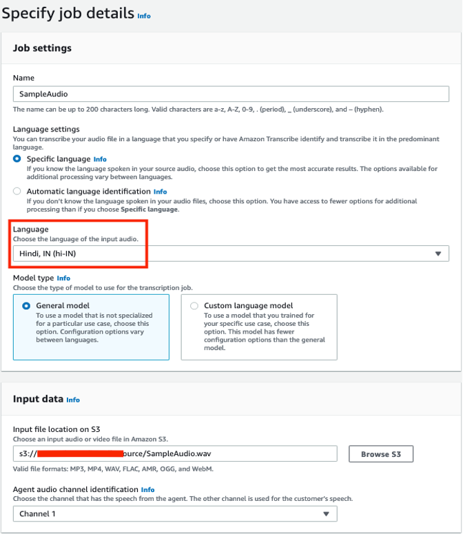
- In the Output data section, leave the defaults.
- In the Access permissions section, select Create an IAM role.
- Create a new AWS Identity and Access Management (IAM) role named HindiTranscription that provides Amazon Transcribe service permissions to read the audio files from the S3 bucket and use the AWS Key Management Service (AWS KMS) key to decrypt.

- In the Configure job section, leave the defaults, including Custom vocabulary deselected.
- Choose Create job to transcribe the audio file.

When the status of the job is Complete, you can review the transcription by choosing the job (SampleAudio).

The customer and the agent sentences are clearly separated out, which helps us identify whether the customer or the agent spoke any specific words or phrases.
Measure model accuracy
Word error rate (WER) is the recommended and most commonly used metric for evaluating the accuracy of Automatic Speech Recognition (ASR) systems. The goal is to reduce the WER as much possible to improve the accuracy of the ASR system.
To calculate WER, complete the following steps. This post uses the open-source asr-evaluation evaluation tool to calculate WER, but other tools such as SCTK or JiWER are also available.
-
Install the
asr-evaluationtool, which makes the wer script available on your command line.
Use a command line on macOS or Linux platforms to run the wer commands shown later in the post. - Copy the transcript from the Amazon Transcribe job details page to a text file named
hypothesis.txt.
When you copy the transcription from the console, you’ll notice a new line character between the wordsAgent :, Customer :,and the Hindi script.
The new line characters have been removed to save space in this post. If you choose to use the text as is from the console, make sure that the reference text file you create also has the new line characters, because the wer tool compares line by line. - Review the entire transcript and identify any words or phrases that need to be corrected:
Customer : हेलो,
Agent : गुड मोर्निग इंडिया ट्रेवल एजेंसी सेम है। लावन्या बात कर रही हूँ किस तरह से मैं आपकी सहायता कर सकती हूँ।
Customer : मैं बहुत दिनों उनसे हैदराबाद ट्रेवल के बारे में सोच रहा था। क्या आप मुझे कुछ अच्छे लोकेशन के बारे में बता सकती हैं?
Agent :हाँ बिल्कुल। हैदराबाद में बहुत सारे प्लेस है। उनमें से चार महीना गोलकुंडा फोर सलार जंग म्यूजियम और बिरला प्लेनेटोरियम मशहूर है।
Customer : हाँ बढिया थैंक यू मैं अगले सैटरडे और संडे को ट्राई करूँगा।
Agent : एक सजेशन वीकेंड में ट्रैफिक ज्यादा रहने के चांसेज है।
Customer : सिरियसली एनी टिप्स चिकन शेर
Agent : आप टेक्सी यूस कर लो ड्रैब और पार्किंग का प्राब्लम नहीं होगा।
Customer : ग्रेट आइडिया थैंक्यू सो मच।The highlighted words are the ones that the default Amazon Transcribe model didn’t render correctly. - Create another text file named
reference.txt, replacing the highlighted words with the desired words you expect to see in the transcription:
Customer : हेलो,
Agent : गुड मोर्निग सौथ इंडिया ट्रेवल एजेंसी से मैं । लावन्या बात कर रही हूँ किस तरह से मैं आपकी सहायता कर सकती हूँ।
Customer : मैं बहुत दिनोंसे हैदराबाद ट्रेवल के बारे में सोच रहा था। क्या आप मुझे कुछ अच्छे लोकेशन के बारे में बता सकती हैं?
Agent : हाँ बिल्कुल। हैदराबाद में बहुत सारे प्लेस है। उनमें से चार मिनार गोलकोंडा फोर्ट सालार जंग म्यूजियम और बिरला प्लेनेटोरियम मशहूर है।
Customer : हाँ बढिया थैंक यू मैं अगले सैटरडे और संडे को ट्राई करूँगा।
Agent : एक सजेशन वीकेंड में ट्रैफिक ज्यादा रहने के चांसेज है।
Customer : सिरियसली एनी टिप्स यू केन शेर
Agent : आप टेक्सी यूस कर लो ड्रैव और पार्किंग का प्राब्लम नहीं होगा।
Customer : ग्रेट आइडिया थैंक्यू सो मच। - Use the following command to compare the reference and hypothesis text files that you created:
You get the following output:
The wer command compares text from the files reference.txt and hypothesis.txt. It reports errors for each sentence and also the total number of errors (WER: 9.848% ( 13 / 132)) in the entire transcript.
From the preceding output, wer reported 13 errors out of 132 words in the transcript. These errors can be of three types:
- Substitution errors – These occur when Amazon Transcribe writes one word in place of another. For example, in our transcript, the word “महीना (Mahina)” was written instead of “मिनार (Minar)” in sentence 4.
- Deletion errors – These occur when Amazon Transcribe misses a word entirely in the transcript.In our transcript, the word “सौथ (South)” was missed in sentence 2.
- Insertion errors – These occur when Amazon Transcribe inserts a word that wasn’t spoken. We don’t see any insertion errors in our transcript.
Observations from the transcript created by the default model
We can make the following observations based on the transcript:
- The total WER is 9.848%, meaning 90.152% of the words are transcribed accurately.
- The default Hindi model transcribed most of the English words accurately. This is because the default model is trained to recognize the most common English words out of the box. The model is also trained to recognize Hinglish language, where English words randomly appear in Hindi conversations. For example:
- गुड मोर्निग – Good morning (sentence 2).
- ट्रेवल एजेंसी – Travel agency (sentence 2).
- ग्रेट आइडिया थैंक्यू सो मच – Great idea thank you so much (sentence 9).
- Sentence 4 has the most errors, which are the names of places in the Indian city Hyderabad:
- हाँ बिल्कुल। हैदराबाद में बहुत सारे प्लेस है। उनमें से चार महीना गोलकुंडा फोर सलार जंग म्यूजियम और बिरला प्लेनेटोरियम मशहूर है।
In the next step, we demonstrate how to correct the highlighted words in the preceding sentence using custom vocabulary in Amazon Transcribe:
- चार महीना (Char Mahina) should be चार मिनार (Char Minar)
- गोलकुंडा फोर (Golcunda Four) should be गोलकोंडा फोर्ट (Golconda Fort)
- सलार जंग (Salar Jung) should be सालार जंग (Saalar Jung)
Train the default model with a custom vocabulary
To create a custom vocabulary, you need to build a text file in a tabular format with the words and phrases to train the default Amazon Transcribe model. Your table must contain all four columns (Phrase, SoundsLike, IPA, and DisplayAs), but the Phrase column is the only one that must contain an entry on each row. You can leave the other columns empty. Each column must be separated by a tab character, even if some columns are left empty. For example, if you leave the IPA and SoundsLike columns empty for a row, the Phrase and DisplaysAs columns in that row must be separated with three tab characters (between Phrase and IPA, IPA and SoundsLike, and SoundsLike and DisplaysAs).
To train the model with a custom vocabulary, complete the following steps:
- Create a file named
HindiCustomVocabulary.txtwith the following content.You can only use characters that are supported for your language. Refer to your language’s character set for details.
The columns contain the following information:
-
Phrase– Contains the words or phrases that you want to transcribe accurately. The highlighted words or phrases in the transcript created by the default Amazon Transcribe model appear in this column. These words are generally acronyms, proper nouns, or domain-specific words and phrases that the default model isn’t aware of. This is a mandatory field for every row in the custom vocabulary table. In our transcript, to correct “गोलकुंडा फोर (Golcunda Four)” from sentence 4, use “गोलकुंडा-फोर (Golcunda-Four)” in this column. If your entry contains multiple words, separate each word with a hyphen (-); do not use spaces. -
IPA– Contains the words or phrases representing speech sounds in the written form. The column is optional; you can leave its rows empty. This column is intended for phonetic spellings using only characters in the International Phonetic Alphabet (IPA). Refer to Hindi character set for the allowed IPA characters for the Hindi language. In our example, we’re not using IPA. If you have an entry in this column, yourSoundsLikecolumn must be empty. -
SoundsLike– Contains words or phrases broken down into smaller pieces (typically based on syllables or common words) to provide a pronunciation for each piece based on how that piece sounds. This column is optional; you can leave the rows empty. Only add content to this column if your entry includes a non-standard word, such as a brand name, or to correct a word that is being incorrectly transcribed. In our transcript, to correct “सलार जंग (Salar Jung)” from sentence 4, use “सा-लार-जंग (Saa-lar-jung)” in this column. Do not use spaces in this column. If you have an entry in this column, yourIPAcolumn must be empty. -
DisplaysAs– Contains words or phrases with the spellings you want to see in the transcription output for the words or phrases in thePhrasefield. This column is optional; you can leave the rows empty. If you don’t specify this field, Amazon Transcribe uses the contents of thePhrasefield in the output file. For example, in our transcript, to correct “गोलकुंडा फोर (Golcunda Four)” from sentence 4, use “गोलकोंडा फोर्ट (Golconda Fort)” in this column.
-
-
Upload the text file (
HindiCustomVocabulary.txt) to an S3 bucket.Now we create a custom vocabulary in Amazon Transcribe. - On the Amazon Transcribe console, choose Custom vocabulary in the navigation pane.
- For Name, enter a name.
- For Language, choose Hindi, IN (hi-IN).
- For Vocabulary input source, select S3 location.
- For Vocabulary file location on S3, enter the S3 path of the
HindiCustomVocabulary.txtfile. - Choose Create vocabulary.

- Transcribe the
SampleAudio.wavfile with the custom vocabulary, with the following parameters:- For Job name , enter
SampleAudioCustomVocabulary. - For Language, choose Hindi, IN (hi-IN).
- For Input file location on S3, browse to the location of
SampleAudio.wav. - For IAM role, select Use an existing IAM role and choose the role you created earlier.
- In the Configure job section, select Custom vocabulary and choose the custom vocabulary
HindiCustomVocabulary.
- For Job name , enter
- Choose Create job.

Measure model accuracy after using custom vocabulary
Copy the transcript from the Amazon Transcribe job details page to a text file named hypothesis-custom-vocabulary.txt:
Customer : हेलो,
Agent : गुड मोर्निग इंडिया ट्रेवल एजेंसी सेम है। लावन्या बात कर रही हूँ किस तरह से मैं आपकी सहायता कर सकती हूँ।
Customer : मैं बहुत दिनों उनसे हैदराबाद ट्रेवल के बारे में सोच रहा था। क्या आप मुझे कुछ अच्छे लोकेशन के बारे में बता सकती हैं?
Agent : हाँ बिल्कुल। हैदराबाद में बहुत सारे प्लेस है। उनमें से चार मिनार गोलकोंडा फोर्ट सालार जंग म्यूजियम और बिरला प्लेनेटोरियम मशहूर है।
Customer : हाँ बढिया थैंक यू मैं अगले सैटरडे और संडे को ट्राई करूँगा।
Agent : एक सजेशन वीकेंड में ट्रैफिक ज्यादा रहने के चांसेज है।
Customer : सिरियसली एनी टिप्स चिकन शेर
Agent : आप टेक्सी यूस कर लो ड्रैब और पार्किंग का प्राब्लम नहीं होगा।
Customer : ग्रेट आइडिया थैंक्यू सो मच।
Note that the highlighted words are transcribed as desired.
Run the wer command again with the new transcript:
You get the following output:
Observations from the transcript created with custom vocabulary
The total WER is 6.061%, meaning 93.939% of the words are transcribed accurately.
Let’s compare the wer output for sentence 4 with and without custom vocabulary. The following is without custom vocabulary:
The following is with custom vocabulary:
There are no errors in sentence 4. The names of the places are transcribed accurately with the help of custom vocabulary, thereby reducing the overall WER from 9.848% to 6.061% for this audio file. This means that the accuracy of transcription improved by nearly 4%.
How custom vocabulary improved the accuracy
We used the following custom vocabulary:
Amazon Transcribe checks if there are any words in the audio file that sound like the words mentioned in the Phrase column. Then the model uses the entries in the IPA, SoundsLike, and DisplaysAs columns for those specific words to transcribe with the desired spellings.
With this custom vocabulary, when Amazon Transcribe identifies a word that sounds like “गोलकुंडा-फोर (Golcunda-Four),” it transcribes that word as “गोलकोंडा फोर्ट (Golconda Fort).”
Recommendations
The accuracy of transcription also depends on parameters like the speakers’ pronunciation, overlapping speakers, talking speed, and background noise. Therefore, we recommend that you to follow the process with a variety of calls (with different customers, agents, interruptions, and so on) that cover the most commonly used domain-specific words for you to build a comprehensive custom vocabulary.
In this post, we learned the process to improve accuracy of transcribing one audio call using custom vocabulary. To process thousands of your contact center call recordings every day, you can use post call analytics, a fully automated, scalable, and cost-efficient end-to-end solution that takes care of most of the heavy lifting. You simply upload your audio files to an S3 bucket, and within minutes, the solution provides call analytics like sentiment in a web UI. Post call analytics provides actionable insights to spot emerging trends, identify agent coaching opportunities, and assess the general sentiment of calls.Post call analytics is an open-source solution that you can deploy using AWS CloudFormation.
Note that custom vocabularies don’t use the context in which the words were spoken, they only focus on individual words that you provide. To further improve the accuracy, you can use custom language models. Unlike custom vocabularies, which associate pronunciation with spelling, custom language models learn the context associated with a given word. This includes how and when a word is used, and the relationship a word has with other words. To create a custom language model, you can use the transcriptions derived from the process we learned for a variety of calls, and combine them with content from your websites or user manuals that contains domain-specific words and phrases.
To achieve the highest transcription accuracy with batch transcriptions, you can use custom vocabularies in conjunction with your custom language models.
Conclusion
In this post, we provided detailed steps to accurately process Hindi audio files containing English words using call analytics and custom vocabularies in Amazon Transcribe. You can use these same steps to process audio calls with any language supported by Amazon Transcribe.
After you derive the transcriptions with your desired accuracy, you can improve your agent-customer conversations by training your agents. You can also understand your customer sentiments and trends. With the help of speaker diarization, loudness detection, and vocabulary filtering features in the call analytics, you can identify whether it was the agent or customer who raised their tone or spoke any specific words. You can categorize calls based on domain-specific words, capture actionable insights, and run analytics to improve your products. Finally, you can translate your transcripts to English or other supported languages of your choice using Amazon Translate.
About the Authors
 Sarat Guttikonda is a Sr. Solutions Architect in AWS World Wide Public Sector. Sarat enjoys helping customers automate, manage, and govern their cloud resources without sacrificing business agility. In his free time, he loves building Legos with his son and playing table tennis.
 Lavanya Sood is a Solutions Architect in AWS World Wide Public Sector based out of New Delhi, India. Lavanya enjoys learning new technologies and helping customers in their cloud adoption journey. In her free time, she loves traveling and trying different foods.
Pinch-grasping robot handles items with precision
Preliminary tests show a prototype pinch-grasping robot achieved a 10-fold reduction in damage on items such as books and boxes.Read More
Detect audio events with Amazon Rekognition
When most people think of using machine learning (ML) with audio data, the use case that usually comes to mind is transcription, also known as speech-to-text. However, there are other useful applications, including using ML to detect sounds.
Using software to detect a sound is called audio event detection, and it has a number of applications. For example, suppose you want to monitor the sounds from a noisy factory floor, listening for an alarm bell that indicates a problem with a machine. In a healthcare environment, you can use audio event detection to passively listen for sounds from a patient that indicate an acute health problem. Media workloads are a good fit for this technique, for example to detect when a referee’s whistle is blown in a sports video. And of course, you can use this technique in a variety of surveillance workloads, like listening for a gunshot or the sound of a car crash from a microphone mounted above a city street.
This post describes how to detect sounds in an audio file even if there are significant background sounds happening at the same time. What’s more, perhaps surprisingly, we use computer vision-based techniques to do the detection, using Amazon Rekognition.
Using audio data with machine learning
The first step in detecting audio events is understanding how audio data is represented. For the purposes of this post, we deal only with recorded audio, although these techniques work with streaming audio.
Recorded audio is typically stored as a sequence of sound samples, which measure the intensity of the sound waves that struck the microphone during recording, over time. There are a wide variety of formats with which to store these samples, but a common approach is to store 10,000, 20,000, or even 40,000 samples per second, with each sample being an integer from 0–65535 (two bytes). Because each sample measures only the intensity of sound waves at a particular moment, the sound data generally isn’t helpful for ML processes because it doesn’t have any useful features in its raw state.
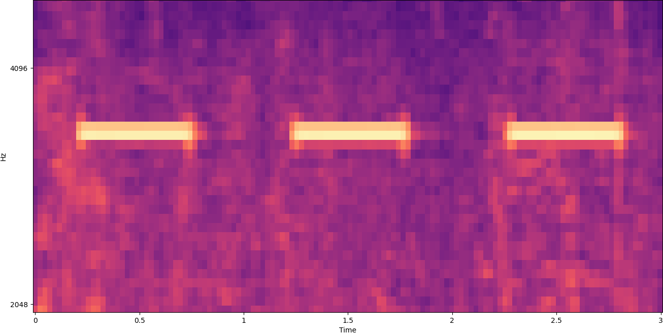
To make that data useful, the sound sample is converted into an image called a spectrogram, which is a representation of the audio data that shows the intensity of different frequency bands over time. The following image shows an example.

The X axis of this image represents time, meaning that the left edge of the image is the very start of the sound, and the right edge of the image is the end. Each column of data within the image represents different frequency bands (indicated by the scale on the left side of the image), and the color at each point represents the intensity of that frequency at that moment in time.
Vertical scaling for spectrograms can be changed to other representations. For example, linear scaling means that the Y axis is evenly divided over frequencies, logarithmic scaling uses a log scale, and so forth. The problem with using these representations is that the frequencies in a sound file are usually not evenly distributed, so most of the information we might be interested in ends up being clustered near the bottom of the image (the lower frequencies).
To solve that problem, our sample image is an example of a Mel spectrogram, which is scaled to closely approximate how human beings perceive sound. Notice the frequency indicators along the left side of the image—they give an idea of how they are distributed vertically, and it’s clear that it’s a non-linear scale.
Additionally, we can modify the measurement of intensity by frequency by time to enhance various features of the audio being measured. As with the Y axis scaling that is implemented by a Mel spectrogram, others emphasize features such as the intensity of the 12 distinctive pitch classes that are used to study music (chroma). Another class emphasizes horizonal (harmonic) features or vertical (percussive) features. The type of sound that is being detected should drive the type of spectrogram used for the detection system.
The earlier example spectrogram represents a music clip that is just over 2 minutes long. Zooming in reveals more detail, as is shown in the following image.

The numbers along the top of the image show the number of seconds from the start of the audio file. You can clearly see a sequence of sounds that seems to repeat more than four times per second, indicated by the bright colors near the bottom of the image.
As you can see, this is one of the benefits of converting audio to a spectrogram—distinct sounds are often easily visible with the naked eye, and even if they aren’t, they can frequently be detected using computer vision object detection algorithms. In fact, this is exactly the process we follow in order to detect sounds.
Looking for discrete sounds in a spectrogram
Depending on the length of the audio file that we’re searching, finding a discrete sound that lasts just a second or two is a challenge. Refer to the first spectrogram we shared—because we’re viewing an entire 3:30 minutes of data, details that last only a second or so aren’t visible. We zoomed in a great deal in order to see the rhythm that is shown in the second image. Clearly, with larger sound files (and therefore much larger spectrograms), we quickly run into problems unless we use a different approach. That approach is called windowing.
Windowing refers to using a sliding window that moves across the entire spectrogram, isolating a few seconds (or less) at a time. By repeatedly isolating portions of the overall image, we get smaller images that are searchable for the presence of the sound to be detected. Because each window could result in only part of the image we’re looking for (as in the case of searching for a sound that doesn’t start exactly at the start of a window), windowing is often performed with succeeding windows being overlapped. For example, the first window starts at 0:00 and extends 2 seconds, then the second window starts at 0:01 and extends 2 seconds, and the third window starts at 0:02 and extends 2 seconds, and so on.
Windowing splits a spectrogram image horizontally. We can improve the effectiveness of the detection process by isolating certain frequency bands by cropping or searching only certain vertical parts of the image. For example, if you know that the alarm bell you want to detect creates sounds that range from one specific frequency to another, you can modify the current window to only consider those frequency ranges. That vastly reduces the amount of data to be manipulated, and results in a much faster search. It also improves accuracy, because it’s eliminating possible false positives matches occurring in frequency bands outside of the desired range. The following images compare a full Y axis (left) with a limited Y axis (right).

Full Y Axis |
Limited Y Axis |
Now that we know how to iterate over a spectrogram with a windowing approach and filter to certain frequency bands, the next step is to do the actual search for the sound. For that, we use Amazon Rekognition Custom Labels. The Rekognition Custom Labels feature builds off of the existing capabilities of Amazon Rekognition, which is already trained on tens of millions of images across many categories. Instead of thousands of images, you simply need to upload a small set of training images (typically a few hundred images, but optimal training dataset size should be arrived at experimentally based on the specific use case to avoid under- or over-training the model) that are specific to your use case via the Rekognition Custom Labels console.
If your images are already labeled, Amazon Rekognition training is accessible with just a few clicks. Alternatively, you can label the images directly within the Amazon Rekognition labeling interface, or use Amazon SageMaker Ground Truth to label them for you. When Amazon Rekognition begins training from your image set, it produces a custom image analysis model for you in just a few hours. Behind the scenes, Rekognition Custom Labels automatically loads and inspects the training data, selects the right ML algorithms, trains a model, and provides model performance metrics. You can then use your custom model via the Rekognition Custom Labels API and integrate it into your applications.
Assembling training data and training a Rekognition Custom Labels model
In the GitHub repo associated with this post, you’ll find code that shows how to listen for the sound of a smoke alarm going off, regardless of background noise. In this case, our Rekognition Custom Labels model is a binary classification model, meaning that the results are either “smoke alarm sound was detected” or “smoke alarm sound was not detected.”
To create a custom model, we need training data. That training data is comprised of two main types: environmental sounds, and the sounds you wish to detect (like a smoke alarm going off).
The environmental data should represent a wide variety of soundscapes that are typical for the environment you want to detect the sound in. For example, if you want to detect a smoke alarm sound in a factory environment, start with sounds recorded in that factory environment under a variety of situations (without the smoke alarm sounding, of course).
The sounds you want to detect should be isolated if possible, meaning the recordings should just be the sound itself without any environmental background sounds. For our example, that’s a sound of a smoke alarm going off.
After you’ve collected these sounds, the code in the GitHub repo shows how to combine the environmental sounds with the smoke alarm sounds in various ways (and then convert them to spectrograms) in order to create a number of images that represent the environmental sounds with and without the smoke alarm sounds overlaid on them. The following image is an example of some environmental sounds with a smoke alarm sound (the bright horizontal bars) overlaid on top of it.

The training and test data is stored in an Amazon Simple Storage Service (Amazon S3) bucket. The following directory structure is a good starting point to organize data within the bucket.

The sample code in the GitHub repo allows you to choose how many training images to create. Rekognition Custom Labels doesn’t require a large number of training images. A training set of 200–500 images should be sufficient.
Creating a Rekognition Custom Labels project requires that you specify the URIs of the S3 folder that contains the training data, and (optionally) test data. When specifying the data sources for the training job, one of the options is Automatic labeling, as shown in the following screenshot.

Using this option means that Amazon Rekognition uses the names of the folders as the label names. For our smoke alarm detection use case, the folder structure inside of the train and test folders looks like the following screenshot.
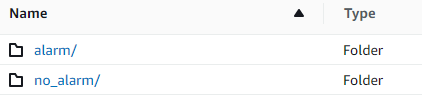
The training data images go into those folders, with spectrograms containing the sound of the smoke alarm going in the alarm folder, and spectrograms that don’t contain the smoke alarm sound in the no_alarm folder. Amazon Rekognition uses those names as the output class names for the custom labels model.
Training a custom label model usually takes 30–90 minutes. At the end of that training, you must start the trained model so it becomes available for use.
End-to-end architecture for sound detection
After we create our model, the next step is to set up an inference pipeline, so we can use the model to detect if a smoke alarm sound is present in an audio file. To do this, the input sound must be turned into a spectrogram and then windowed and filtered by frequency, as was done for the training process. Each window of the spectrogram is given to the model, which returns a classification that indicates if the smoke alarm sounded or not.
The following diagram shows an example architecture that implements this inference pipeline.

This architecture waits for an audio file to be placed into an S3 bucket, which then causes an AWS Lambda function to be invoked. Lambda is a serverless, event-driven compute service that lets you run code for virtually any type of application or backend service without provisioning or managing servers. You can trigger a Lambda function from over 200 AWS services and software as a service (SaaS) applications, and only pay for what you use.
The Lambda function receives the name of the bucket and the name of the key (or file name) of the audio file. The file is downloaded from Amazon S3 to the function’s memory, which then converts it into a spectrogram and performs windowing and frequency filtering. Each windowed portion of the spectrogram is then sent to Amazon Rekognition, which uses the previously-trained Amazon Custom Labels model to detect the sound. If that sound is found, the Lambda function signals that by using an Amazon Simple Notification Service (Amazon SNS) notification. Amazon SNS offers a pub/sub approach where notifications can be sent to Amazon Simple Queue Service (Amazon SQS) queues, Lambda functions, HTTPS endpoints, email addresses, mobile push, and more.
Conclusion
You can use machine learning with audio data to determine when certain sounds occur, even when other sounds are occurring at the same time. Doing so requires converting the sound into a spectrogram image, and then homing in on different parts of that spectrogram by windowing and filtering by frequency band. Rekognition Custom Labels makes it easy to train a custom model for sound detection.
You can use the GitHub repo containing the example code for this post as a starting point for your own experiments. For more information about audio event detection, refer to Sound Event Detection: A Tutorial.
About the authors
 Greg Sommerville is a Senior Prototyping Architect on the AWS Prototyping and Cloud Engineering team, where he helps AWS customers implement innovative solutions to challenging problems with machine learning, IoT and serverless technologies. He lives in Ann Arbor, Michigan and enjoys practicing yoga, catering to his dogs, and playing poker.
 Jeff Harman is a Senior Prototyping Architect on the AWS Prototyping and Cloud Engineering team, where he helps AWS customers implement innovative solutions to challenging problems. He lives in Unionville, Connecticut and enjoys woodworking, blacksmithing, and Minecraft.
A quick guide to Amazon’s 40-plus papers at Interspeech 2022
Speech recognition and text-to-speech predominate, but other topics include audio watermarking, automatic dubbing, and compression.Read More
How The Chefz serves the perfect meal with Amazon Personalize
This is a guest post by Ramzi Alqrainy, Chief Technology Officer, The Chefz.
The Chefz is a Saudi-based online food delivery startup, founded in 2016. At the core of The Chefz’s business model is enabling its customers to order food and sweets from top elite restaurants, bakeries, and chocolate shops. In this post, we explain how The Chefz uses Amazon Personalize filters to apply business rules on recommendations to end-users, increasing revenue by 35%.
Food delivery is a growing industry but at the same time is extremely competitive. The biggest challenge in the industry is maintaining customer loyalty. This requires a comprehensive understanding of the customer’s preferences, the ability to provide excellent response time in terms of on-time delivery, and good food quality. These three factors determine the most important metric for The Chefz’s customer satisfaction. The Chefz’s demands fluctuate, especially with spikes in order volumes at lunch and dinner times. Demand also fluctuates during special days such as Mother’s Day, the football final, Ramadan dusk (Suhoor) and sundown (Iftaar) times, or Eid festive holidays. During these times, the demand can increase by up to 300%, adding one more critical challenge to recommend the perfect meal based on time of the day, especially in Ramadan.
The perfect meal at the right time
To make the ordering process more deterministic and to cater to peak demand times, The Chefz team decided to divide the day into different periods. For example, during Ramadan season, days are divided into Iftar and Suhoor. On regular days, days consist of four periods: breakfast, lunch, dinner, and dessert. The technology that underpins this deterministic ordering process is Amazon Personalize, a powerful recommendation engine. Amazon Personalize takes these grouped periods along with the location of the customer to provide a perfect recommendation.
This ensures the customer receives restaurant and meal recommendations based on their preference and from a nearby location so that it arrives quickly at their doorstep.
This recommendation engine based on Amazon Personalize is the key ingredient in how The Chefz’s customers enjoy personalized restaurant meal recommendations, rather than random recommendations for categories of favorites.
The personalization journey
The Chefz started its personalization journey by offering restaurant recommendations for customers using Amazon Personalize based on previous interactions, user metadata (such as age, nationality, and diet), restaurant metadata like category and food types offered, along with live tracking for customer interactions on the Chefz mobile application and web portal. The initial deployment phases of Amazon Personalize led to a 10% increase in customer interactions with the portal.
Although that was a milestone step, delivery time was still a problem that many customers encountered. One of the main difficulties customers had was delivery time during rush hour. To address this, the data scientist team added location as an additional feature to user metadata so recommendations would take into consideration both user preference and location for improved delivery time.
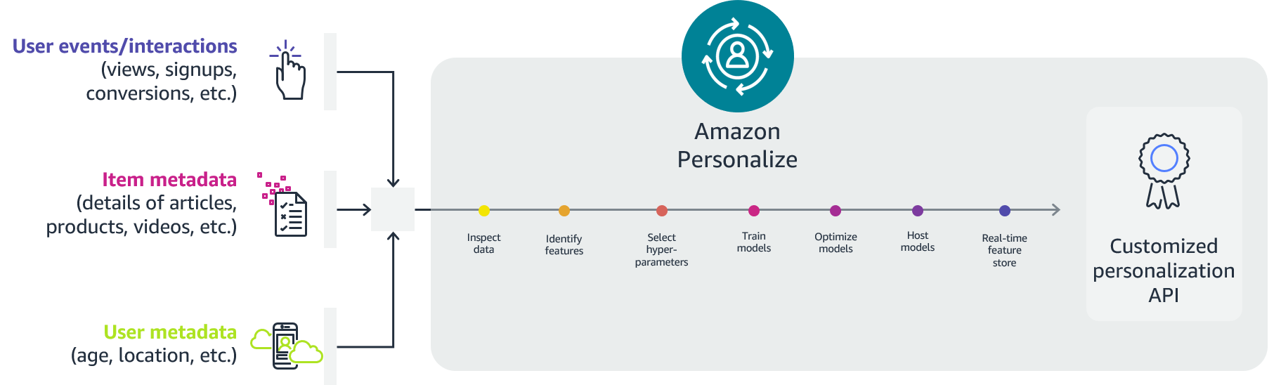
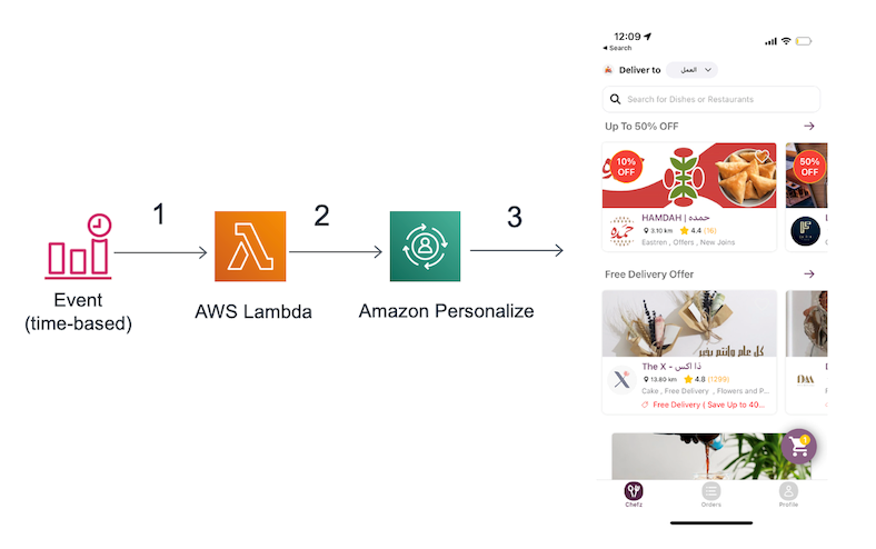
The next step in the recommendation journey was to consider annual timing, especially Ramadan, and the time of day. These considerations ensured The Chefz could recommend heavy meals or restaurants that provide Iftaar meals during Ramadan sundown, and lighter meals in the late evening. To solve this challenge, the data scientist team used Amazon Personalize filters updated by AWS Lambda functions, which were triggered by an Amazon CloudWatch cron job.
The following architecture shows the automated process for applying the filters:
- A CloudWatch event uses a cron expression to schedule when a Lambda function is invoked.
- When the Lambda function is triggered, it attaches the filter to the recommendation engine to apply business rules.
- Recommended meals and restaurants are delivered to end-users on the application.
Conclusion
Amazon Personalize enabled The Chefz to apply context about individual customers and their circumstances, and deliver customized recommendations based on business rules such as special deals and offers through our mobile application. This increased revenue by 35% per month and doubled customer orders at recommended restaurants.
“The customer is at the heart of everything we do at The Chefz, and we’re working tirelessly to improve and enhance their experience. With Amazon Personalize, we are able to achieve personalization at scale across our entire customer base, which was previously impossible.”
-Ramzi Algrainy, CTO at The Chefz.
About the authors
 Ramzi Alqrainy is Chief Technology Officer at The Chefz. Ramzi is a contributor to Apache Solr and Slack and technical reviewer, and has published many papers in IEEE focusing on search and data functions.
 Mohamed Ezzat is a Senior Solutions Architect at AWS with a focus in machine learning. He works with customers to address their business challenges using cloud technologies. Outside of work, he enjoys playing table tennis.
Distributed training with Amazon EKS and Torch Distributed Elastic
Distributed deep learning model training is becoming increasingly important as data sizes are growing in many industries. Many applications in computer vision and natural language processing now require training of deep learning models, which are growing exponentially in complexity and are often trained with hundreds of terabytes of data. It then becomes important to use a vast cloud infrastructure to scale the training of such large models.
Developers can use open-source frameworks such as PyTorch to easily design intuitive model architectures. However, scaling the training of these models across multiple nodes can be challenging due to increased orchestration complexity.
Distributed model training mainly consists of two paradigms:
- Model parallel – In model parallel training, the model itself is so large that it can’t fit in the memory of a single GPU, and multiple GPUs are needed to train the model. The Open AI’s GPT-3 model with 175 billion trainable parameters (approximately 350 GB in size) is a good example of this.
- Data parallel – In data parallel training, the model can reside in a single GPU, but because the data is so large, it can take days or weeks to train a model. Distributing the data across multiple GPU nodes can significantly reduce the training time.
In this post, we provide an example architecture to train PyTorch models using the Torch Distributed Elastic framework in a distributed data parallel fashion using Amazon Elastic Kubernetes Service (Amazon EKS).
Prerequisites
To replicate the results reported in this post, the only prerequisite is an AWS account. In this account, we create an EKS cluster and an Amazon FSx for Lustre file system. We also push container images to an Amazon Elastic Container Registry (Amazon ECR) repository in the account. Instructions to set up these components are provided as needed throughout the post.
EKS clusters
Amazon EKS is a managed container service to run and scale Kubernetes applications on AWS. With Amazon EKS, you can efficiently run distributed training jobs using the latest Amazon Elastic Compute Cloud (Amazon EC2) instances without needing to install, operate, and maintain your own control plane or nodes. It is a popular orchestrator for machine learning (ML) and AI workflows. A typical EKS cluster in AWS looks like the following figure.

We have released an open-source project, AWS DevOps for EKS (aws-do-eks), which provides a large collection of easy-to-use and configurable scripts and tools to provision EKS clusters and run distributed training jobs. This project is built following the principles of the Do Framework: Simplicity, Flexibility, and Universality. You can configure your desired cluster by using the eks.conf file and then launch it by running the eks-create.sh script. Detailed instructions are provided in the GitHub repo.
Train PyTorch models using Torch Distributed Elastic
Torch Distributed Elastic (TDE) is a native PyTorch library for training large-scale deep learning models where it’s critical to scale compute resources dynamically based on availability. The TorchElastic Controller for Kubernetes is a native Kubernetes implementation for TDE that automatically manages the lifecycle of the pods and services required for TDE training. It allows for dynamically scaling compute resources during training as needed. It also provides fault-tolerant training by recovering jobs from node failure.
In this post, we discuss the steps to train PyTorch EfficientNet-B7 and ResNet50 models using ImageNet data in a distributed fashion with TDE. We use the PyTorch DistributedDataParallel API and the Kubernetes TorchElastic controller, and run our training jobs on an EKS cluster containing multiple GPU nodes. The following diagram shows the architecture diagram for this model training.
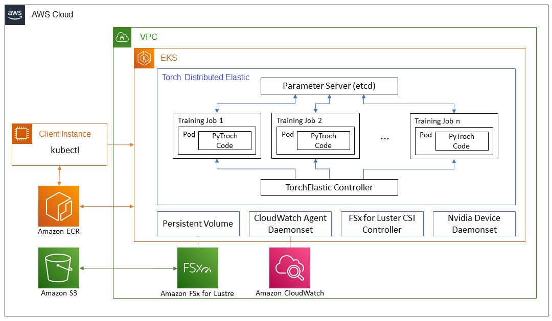
TorchElastic for Kubernetes consists mainly of two components: the TorchElastic Kubernetes Controller (TEC) and the parameter server (etcd). The controller is responsible for monitoring and managing the training jobs, and the parameter server keeps track of the worker nodes for distributed synchronization and peer discovery.
In order for the training pods to access the data, we need a shared data volume that can be mounted by each pod. Some options for shared volumes through Container Storage Interface (CSI) drivers included in AWS DevOps for EKS are Amazon Elastic File System (Amazon EFS) and FSx for Lustre.
Cluster setup
In our cluster configuration, we use one c5.2xlarge instance for system pods. We use three p4d.24xlarge instances as worker pods to train an EfficientNet model. For ResNet50 training, we use p3.8xlarge instances as worker pods. Additionally, we use an FSx shared file system to store our training data and model artifacts.
AWS p4d.24xlarge instances are equipped with Elastic Fabric Adapter (EFA) to provide networking between nodes. We discuss EFA more later in the post. To enable communication through EFA, we need to configure the cluster setup through a .yaml file. An example file is provided in the GitHub repository.
After this .yaml file is properly configured, we can launch the cluster using the script provided in the GitHub repo:
Refer to the GitHub repo for detailed instructions.
There is practically no difference between running jobs on p4d.24xlarge and p3.8xlarge. The steps described in this post work for both. The only difference is the availability of EFA on p4d.24xlarge instances. For smaller models like ResNet50, standard networking compared to EFA networking has minimal impact on the speed of training.
FSx for Lustre file system
FSx is designed for high-performance computing workloads and provides sub-millisecond latency using solid-state drive storage volumes. We chose FSx because it provided better performance as we scaled to a large number of nodes. An important detail to note is that FSx can only exist in a single Availability Zone. Therefore, all nodes accessing the FSx file system should exist in the same Availability Zone as the FSx file system. One way to achieve this is to specify the relevant Availability Zone in the cluster .yaml file for the specific node groups before creating the cluster. Alternatively, we can modify the network part of the auto scaling group for these nodes after the cluster is set up, and limit it to using a single subnet. This can be easily done on the Amazon EC2 console.
Assuming that the EKS cluster is up and running, and the subnet ID for the Availability Zone is known, we can set up an FSx file system by providing the necessary information in the fsx.conf file as described in the readme and running the deploy.sh script in the fsx folder. This sets up the correct policy and security group for accessing the file system. The script also installs the CSI driver for FSx as a daemonset. Finally, we can create the FSx persistent volume claim in Kubernetes by applying a single .yaml file:
This creates an FSx file system in the Availability Zone specified in the fsx.conf file, and also creates a persistent volume claim fsx-pvc, which can be mounted by any of the pods in the cluster in a read-write-many (RWX) fashion.
In our experiment, we used complete ImageNet data, which contains more that 12 million training images divided into 1,000 classes. The data can be downloaded from the ImageNet website. The original TAR ball has several directories, but for our model training, we’re only interested in ILSVRC/Data/CLS-LOC/, which includes the train and val subdirectories. Before training, we need to rearrange the images in the val subdirectory to match the directory structure required by the PyTorch ImageFolder class. This can be done using a simple Python script after the data is copied to the persistent volume in the next step.
To copy the data from an Amazon Simple Storage Service (Amazon S3) bucket to the FSx file system, we create a Docker image that includes scripts for this task. An example Dockerfile and a shell script are included in the csi folder within the GitHub repo. We can build the image using the build.sh script and then push it to Amazon ECR using the push.sh script. Before using these scripts, we need to provide the correct URI for the ECR repository in the .env file in the root folder of the GitHub repo. After we push the Docker image to Amazon ECR, we can launch a pod to copy the data by applying the relevant .yaml file:
The pod automatically runs the script data-prep.sh to copy the data from Amazon S3 to the shared volume. Because the ImageNet data has more than 12 million files, the copy process takes a couple of hours. The Python script imagenet_data_prep.py is also run to rearrange the val dataset as expected by PyTorch.
Network acceleration
We can use Elastic Fabric Adapter (EFA) in combination with supported EC2 instance types to accelerate network traffic between the GPU nodes in your cluster. This can be useful when running large distributed training jobs where standard network communication may be a bottleneck. Scripts to deploy and test the EFA device plugin in the EKS cluster that we use here are included in the efa-device-plugin folder in the GitHub repo. To enable a job with EFA in your EKS cluster, in addition to the cluster nodes having the necessary hardware and software, the EFA device plugin needs to be deployed to the cluster, and your job container needs to have compatible CUDA and NCCL versions installed.
To demonstrate running NCCL tests and evaluating the performance of EFA on p4d.24xlarge instances, we first must deploy the Kubeflow MPI operator by running the corresponding deploy.sh script in the mpi-operator folder. Then we run the deploy.sh script and update the test-efa-nccl.yaml manifest so limits and requests for resource vpc.amazonaws.com are set to 4. The four available EFA adapters in the p4d.24xlarge nodes get bundled together to provide maximum throughput.
Run kubectl apply -f ./test-efa-nccl.yaml to apply the test and then display the logs of the test pod. The following line in the log output confirms that EFA is being used:
The test results should look similar to the following output:
We can observe in the test results that the max throughput is about 42 GB/sec and average bus bandwidth is approximately 8 GB.
We also conducted experiments with a single EFA adapter enabled as well as no EFA adapters. All results are summarized in the following table.
| Number of EFA Adapters | Net/OFI Selected Provider | Avg. Bandwidth (GB/s) | Max. Bandwith (GB/s) |
| 4 | efa | 8.24 | 42.04 |
| 1 | efa | 3.02 | 5.89 |
| 0 | socket | 0.97 | 2.38 |
We also found that for relatively small models like ImageNet, the use of accelerated networking reduces the training time per epoch only with 5–8% at batch size of 64. For larger models and smaller batch sizes, when increased network communication of weights is needed, the use of accelerated networking has greater impact. We observed a decrease of epoch training time with 15–18% for training of EfficientNet-B7 with batch size 1. The actual impact of EFA on your training will depend on the size of your model.
GPU monitoring
Before running the training job, we can also set up Amazon CloudWatch metrics to visualize the GPU utilization during training. It can be helpful to know whether the resources are being used optimally or potentially identify resource starvation and bottlenecks in the training process.
The relevant scripts to set up CloudWatch are located in the gpu-metrics folder. First, we create a Docker image with amazon-cloudwatch-agent and nvidia-smi. We can use the Dockerfile in the gpu-metrics folder to create this image. Assuming that the ECR registry is already set in the .env file from the previous step, we can build and push the image using build.sh and push.sh. After this, running the deploy.sh script automatically completes the setup. It launches a daemonset with amazon-cloudwatch-agent and pushes various metrics to CloudWatch. The GPU metrics appear under the CWAgent namespace on the CloudWatch console. The rest of the cluster metrics show under the ContainerInsights namespace.
Model training
All the scripts needed for PyTorch training are located in the elasticjob folder in the GitHub repo. Before launching the training job, we need to run the etcd server, which is used by the TEC for worker discovery and parameter exchange. The deploy.sh script in the elasticjob folder does exactly that.
To take advantage of EFA in p4d.24xlarge instances, we need to use a specific Docker image available in the Amazon ECR Public Gallery that supports NCCL communication through EFA. We just need to copy our training code to this Docker image. The Dockerfile under the samples folder creates an image to be used when running training job on p4d instances. As always, we can use the build.sh and push.sh scripts in the folder to build and push the image.
The imagenet-efa.yaml file describes the training job. This .yaml file sets up the resources needed for running the training job and also mounts the persistent volume with the training data set up in the previous section.
A couple of things are worth pointing out here. The number of replicas should be set to the number of nodes available in the cluster. In our case, we set this to 3 because we had three p4d.24xlarge nodes. In the imagenet-efa.yaml file, the nvidia.com/gpu parameter under resources and nproc_per_node under args should be set to the number of GPUs per node, which in the case of p4d.24xlarge is 8. Also, the worker argument for the Python script sets the number of CPUs per process. We chose this to be 4 because, in our experiments, this provides optimal performance when running on p4d.24xlarge instances. These settings are necessary in order to maximize the use of all the hardware resources available in the cluster.
When the job is running, we can observe the GPU usage in CloudWatch for all the GPUs in the cluster. The following is an example from one of our training jobs with three p4d.24xlarge nodes in the cluster. Here we’ve selected one GPU from each node. With the settings mentioned earlier, the GPU usage is close to 100% during the training phase of the epoch for all of the nodes in the cluster.

For training a ResNet50 model using p3.8xlarge instances, we need exactly the same steps as described for the EfficientNet training using p4d.24xlarge. We can also use the same Docker image. As mentioned earlier, p3.8xlarge instances aren’t equipped with EFA. However, for the ResNet50 model, this is not a significant drawback. The imagenet-fsx.yaml script provided in the GitHub repository sets up the training job with appropriate resources for the p3.8xlarge node type. The job uses the same dataset from the FSx file system.
GPU scaling
We ran some experiments to observe how the training time scales for the EfficientNet-B7 model by increasing the number of GPUs. To do this, we changed the number of replicas from 1 to 3 in our training .yaml file for each training run. We only observed the time for a single epoch while using the complete ImageNet dataset. The following figure shows the results for our GPU scaling experiment. The red dotted line represents how the training time should go down from a run using 8 GPUs by increasing the number of GPUs. As we can see, the scaling is quite close to what is expected.

Similarly, we obtained the GPU scaling plot for ResNet50 training on p3.8xlarge instances. For this case, we changed the replicas in our .yaml file from 1 to 4. The results of this experiment are shown in the following figure.

Clean up
It’s important to spin down resources after model training in order to avoid costs associated with running idle instances. With each script that creates resources, the GitHub repo provides a matching script to delete them. To clean up our setup, we must delete the FSx file system before deleting the cluster because it’s associated with a subnet in the cluster’s VPC. To delete the FSx file system, we just need to run the following command (from inside the fsx folder):
Note that this will not only delete the persistent volume, it will also delete the FSx file system, and all the data on the file system will be lost. When this step is complete, we can delete the cluster by using the following script in the eks folder:
This will delete all the existing pods, remove the cluster, and delete the VPC created in the beginning.
Conclusion
In this post, we detailed the steps needed for running PyTorch distributed data parallel model training on EKS clusters. This task may seem daunting, but the AWS DevOps for EKS project created by the ML Frameworks team at AWS provides all the necessary scripts and tools to simplify the process and make distributed model training easily accessible.
For more information on the technologies used in this post, visit Amazon EKS and Torch Distributed Elastic. We encourage you to apply the approach described here to your own distributed training use cases.
Resources
- Amazon EC2 Instance Types
- Machine Learning on Amazon EKS
- Running TorchServe on Amazon Elastic Kubernetes Service
- Distributed Model Training Workshop for AWS EKS
About the authors
 Imran Younus is a Principal Solutions Architect for ML Frameworks team at AWS. He focuses on large scale machine learning and deep learning workloads across AWS services like Amazon EKS and AWS ParallelCluster. He has extensive experience in applications of Deep Leaning in Computer Vision and Industrial IoT. Imran obtained his PhD in High Energy Particle Physics where he has been involved in analyzing experimental data at peta-byte scales.
 Alex Iankoulski is a full-stack software and infrastructure architect who likes to do deep, hands-on work. He is currently a Principal Solutions Architect for Self-managed Machine Learning at AWS. In his role he focuses on helping customers with containerization and orchestration of ML and AI workloads on container-powered AWS services. He is also the author of the open source Do framework and a Docker captain who loves applying container technologies to accelerate the pace of innovation while solving the world’s biggest challenges. During the past 10 years, Alex has worked on combating climate change, democratizing AI and ML, making travel safer, healthcare better, and energy smarter.
Model assesses the validity of tips offered in product reviews
Method would enable customers to evaluate supporting evidence for tip reliability.Read More
Learn How Amazon SageMaker Clarify Helps Detect Bias
Bias detection in data and model outcomes is a fundamental requirement for building responsible artificial intelligence (AI) and machine learning (ML) models. Unfortunately, detecting bias isn’t an easy task for the vast majority of practitioners due to the large number of ways in which it can be measured and different factors that can contribute to a biased outcome. For instance, an imbalanced sampling of the training data may result in a model that is less accurate for certain subsets of the data. Bias may also be introduced by the ML algorithm itself—even with a well-balanced training dataset, the outcomes might favor certain subsets of the data as compared to the others.
To detect bias, you must have a thorough understanding of different types of bias and the corresponding bias metrics. For example, at the time of this writing, Amazon SageMaker Clarify offers 21 different metrics to choose from.
In this post, we use an income prediction use case (predicting user incomes from input features like education and number of hours worked per week) to demonstrate different types of biases and the corresponding metrics in SageMaker Clarify. We also develop a framework to help you decide which metrics matter for your application.
Introduction to SageMaker Clarify
ML models are being increasingly used to help make decisions across a variety of domains, such as financial services, healthcare, education, and human resources. In many situations, it’s important to understand why the ML model made a specific prediction and also whether the predictions were impacted by bias.
SageMaker Clarify provides tools for both of these needs, but in this post we only focus on the bias detection functionality. To learn more about explainability, check out Explaining Bundesliga Match Facts xGoals using Amazon SageMaker Clarify.
SageMaker Clarify is a part of Amazon SageMaker, which is a fully managed service to build, train, and deploy ML models.
Examples of questions about bias
To ground the discussion, the following are some sample questions that ML builders and their stakeholders may have regarding bias. The list consists of some general questions that may be relevant for several ML applications, as well as questions about specific applications like document retrieval.
You might ask, given the groups of interest in the training data (for example, men vs. women) which metrics should I use to answer the following questions:
- Does the group representation in the training data reflect the real world?
- Do the target labels in the training data favor one group over the other by assigning it more positive labels?
- Does the model have different accuracy for different groups?
- In a model whose purpose is to identify qualified candidates for hiring, does the model have the same precision for different groups?
- In a model whose purpose is to retrieve documents relevant to an input query, does the model retrieve relevant documents from different groups in the same proportion?
In the rest of this post, we develop a framework for how to consider answering these questions and others through the metrics available in SageMaker Clarify.
Use case and context
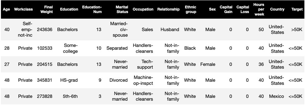
This post uses an existing example of a SageMaker Clarify job from the Fairness and Explainability with SageMaker Clarify notebook and explains the generated bias metric values. The notebook trains an XGBoost model on the UCI Adult dataset (Dua, D. and Graff, C. (2019). UCI Machine Learning Repository. Irvine, CA: University of California, School of Information and Computer Science).
The ML task in this dataset is to predict whether a person has a yearly income of more or less than $50,000. The following table shows some instances along with their features. Measuring bias in income prediction is important because we could use these predictions to inform decisions like discount offers and targeted marketing.
Bias terminology
Before diving deeper, let’s review some essential terminology. For a complete list of terms, see Amazon SageMaker Clarify Terms for Bias and Fairness.
- Label – The target feature that the ML model is trained to predict. An observed label refers to the label value observed in the data used to train or test the model. A predicted label is the value predicted by the ML model. Labels could be binary, and are often encoded as 0 and 1. We assume 1 to represent a favorable or positive label (for example, income more than or equal to $50,000), and 0 to represent an unfavorable or negative label. Labels could also consist of more than two values. Even in these cases, one or more of the values constitute favorable labels. For the sake of simplicity, this post only considers binary labels. For details on handling labels with more than two values and labels with continuous values (for example, in regression), see Amazon AI Fairness and Explainability Whitepaper.
-
Facet – A column or feature with respect to which bias is measured. In our example, the facet is
sexand takes two values:womanandman, encoded asfemaleandmalein the data (this data is extracted from the 1994 Census and enforces a binary option). Although the post considers a single facet with only two values, for more complex cases involving multiple facets or facets with more than two values, see Amazon AI Fairness and Explainability Whitepaper. -
Bias – A significant imbalance in the input data or model predictions across different facet values. What constitutes “significant” depends on your application. For most metrics, a value of 0 implies no imbalance. Bias metrics in SageMaker Clarify are divided into two categories:
- Pretraining – When present, pretraining bias indicates imbalances in the data only.
- Posttraining – Posttraining bias additionally considers the predictions of the models.
Let’s examine each category separately.
Pretraining bias
Pretraining bias metrics in SageMaker Clarify answer the following question: Do all facet values have equal (or similar) representation in the data? It’s important to inspect the data for pretraining bias because it may translate into posttraining bias in the model predictions. For instance, a model trained on imbalanced data where one facet value appears very rarely can exhibit substantially worse accuracy for that facet value. Equal representation can be calculated over the following:
- The whole training data irrespective of the labels
- The subset of the training data with positive labels only
- Each label separately
The following figure provides a summary of how each metric fits into each of the three categories.
Some categories consist of more than one metric. The basic metrics (grey boxes) answer the question about bias in that category in the simplest form. Metrics in white boxes additionally cover special cases (for example, Simpson’s paradox) and user preferences (for example, focusing on certain parts of the population when computing predictive performance).
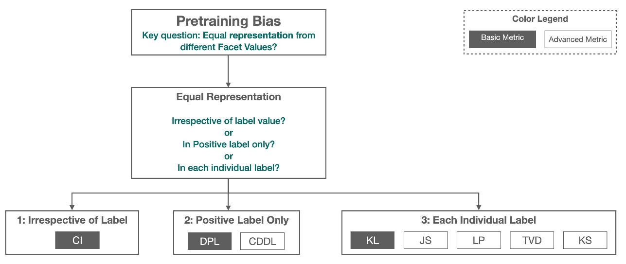
Facet value representation irrespective of labels
The only metric in this category is Class Imbalance (CI). The goal of this metric is to measure if all the facet values have equal representation in the data.
CI is the difference in the fraction of the data constituted by the two facet values. In our example dataset, for the facet sex, the breakdown (shown in the pie chart) shows that women constitute 32.4% of the training data, whereas men constitute 67.6%. As a result:
CI = 0.676 - 0.324 = 0.352
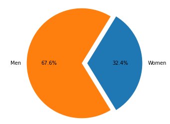
A severely high class imbalance could lead to worse predictive performance for the facet value with smaller representation.
Facet value representation at the level of positive labels only
Another way to measure equal representation is to check whether all facet values contain a similar fraction of samples with positive observed labels. Positive labels consist of favorable outcomes (for example, loan granted, selected for the job), so analyzing positive labels separately helps assess if the favorable decisions are distributed evenly.
In our example dataset, the observed labels break down into positive and negative values, as shown in the following figure.
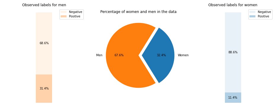
11.4% of all women and 31.4% of all men have the positive label (dark shaded region in the left and right bars). The Difference in Positive Proportions in Labels (DPL) measures this difference.
DPL = 0.314 - 0.114 = 0.20
The advanced metric in this category, Conditional Demographic Disparity in Labels (CDDL), measures the differences in the positive labels, but stratifies them with respect to another variable. This metric helps control for the Simpson’s paradox, a case where a computation over the whole data shows bias, but the bias disappears when grouping the data with respect to some side-information.
The 1973 UC Berkeley Admissions Study provides an example. According to the data, men were admitted at a higher rate than women. However, when examined at the level of individual university departments, women were admitted at similar or higher rate at each department. This observation can be explained by the Simpson’s paradox, which arose here because women applied to schools that were more competitive. As a result, fewer women were admitted overall compared to men, even though school by school they were admitted at a similar or higher rate.
For more detail on how CDDL is computed, see Amazon AI Fairness and Explainability Whitepaper.
Facet value representation at the level of each label separately
Equality in representation can also be measured for each individual label, not just the positive label.
Metrics in this category compute the difference in the label distribution of different facet values. The label distribution for a facet value contains all the observed label values, along with the fraction of samples with that label’s value. For instance, in the figure showing labels distributions, 88.6% of women have a negative observed label and 11.4% have a positive observed label. So the label distribution for women is [0.886, 0.114] and for men is [0.686, 0.314].
The basic metric in this category, Kullback-Leibler divergence (KL), measures this difference as:
KL = [0.686 x log(0.686/0.886)] + [0.314 x log(0.314/0.114)] = 0.143
The advanced metrics in this category, Jensen-Shannon divergence (JS), Lp-norm (LP), Total Variation Distance (TVD), and Kolmogorov-Smirnov (KS), also measure the difference between the distributions but have different mathematical properties. Barring special cases, they will deliver insights similar to KL. For example, although the KL value can be infinity when a facet value contains no samples with a certain labels (for example, no men with a negative label), JS avoids these infinite values. For more detail into these differences, see Amazon AI Fairness and Explainability Whitepaper.
Relationship between DPL (Category 2) and distribution-based metrics of KL/JS/LP/TVD/KS (Category 3)
Distribution-based metrics are more naturally applicable to non-binary labels. For binary labels, owing to the fact that imbalance in the positive label can be used to compute the imbalance in negative label, the distribution metrics deliver the same insights as DPL. Therefore, you can just use DPL in such cases.
Posttraining bias
Posttraining bias metrics in SageMaker Clarify help us answer two key questions:
- Are all facet values represented at a similar rate in positive (favorable) model predictions?
- Does the model have similar predictive performance for all facet values?
The following figure shows how the metrics map to each of these questions. The second question can be further broken down depending on which label the performance is measured with respect to.
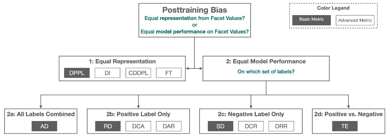
Equal representation in positive model predictions
Metrics in this category check if all facet values contain a similar fraction of samples with positive predicted label by the model. This class of metrics is very similar to the pretraining metrics of DPL and CDDL—the only difference is that this category considers predicted labels instead of observed labels.
In our example dataset, 4.5% of all women are assigned the positive label by the model, and 13.7% of all men are assigned the positive label.
The basic metric in this category, Difference in Positive Proportions in Predicted Labels (DPPL), measures the difference in the positive class assignments.
DPPL = 0.137 - 0.045 = 0.092
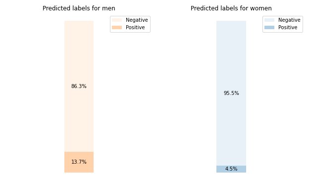
Notice how in the training data, a higher fraction of men had a positive observed label. In a similar manner, a higher fraction of men are assigned a positive predicted label.
Moving on to the advanced metrics in this category, Disparate Impact (DI) measures the same disparity in positive class assignments, but instead of the difference, it computes the ratio:
DI = 0.045 / 0.137 = 0.328
Both DI and DPPL convey qualitatively similar insights but differ at some corner cases. For instance, ratios tend to explode to very large numbers if the denominator is small. Take an example of the numbers 0.1 and 0.0001. The ratio is 0.1/0.0001 = 10,000 whereas the difference is 0.1 – 0.0001 ≈ 0.1. Unlike the other metrics where a value of 0 implies no bias, for DI, no bias corresponds to a value of 1.
Conditional Demographic Disparity in Predicted Labels (CDDPL) measures the disparity in facet value representation in the positive label, but just like the pretraining metric of CDDL, it also controls for the Simpson’s paradox.
Counterfactual Fliptest (FT) measures if similar samples from the two facet values receive similar decisions from the model. A model assigning different decisions to two samples that are similar to each other but differ in the facet values could be considered biased against the facet value being assigned the unfavorable (negative) label. Given the first facet value (women), it assesses whether similar members with the other facet value (men) have a different model prediction. Similar members are chosen based on the k-nearest neighbor algorithm.
Equal performance
The model predictions might have similar representation in positive labels from different facet values, yet the model performance on these groups might significantly differ. In many applications, having a similar predictive performance across different facet values can be desirable. The metrics in this category measure the difference in predictive performance across facet values.
Because the data can be sliced in many different ways based on the observed or predicted labels, there are many different ways to measure predictive performance.
Equal predictive performance irrespective of labels
You could consider the model performance on the whole data, irrespective of the observed or the predicted labels – that is, the overall accuracy.
The following figures shows how the model classifies inputs from the two facet values in our example dataset. True negatives (TN) are cases where both the observed and predicted label were 0. False positives (FP) are misclassifications where the observed label was 0 but the predicted label was 1. True positives (TP) and false negatives (FN) are defined similarly.
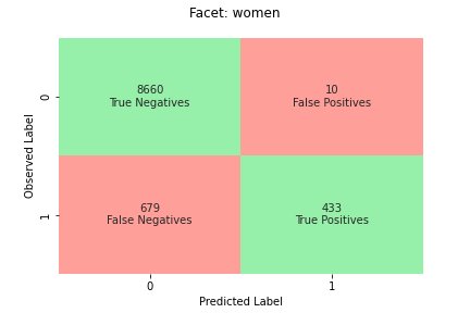 |
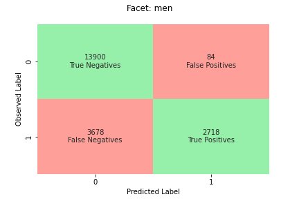 |
For each facet value, the overall model performance, that is, the accuracy for that facet value, is:
Accuracy = (TN + TP) / (TN + FP + FN + TP)
With this formula, the accuracy for women is 0.930 and for men is 0.815. This leads to the only metric in this category, Accuracy Difference (AD):
AD = 0.815 - 0.930 = -0.115
AD = 0 means that the accuracy for both groups is the same. Larger (positive or negative) values indicate larger differences in accuracy.
Equal performance on positive labels only
You could restrict the model performance analysis to positive labels only. For instance, if the application is about detecting defects on an assembly line, it may be desirable to check that non-defective parts (positive label) of different kinds (facet values) are classified as non-defective at the same rate. This quantity is referred to as recall, or true positive rate:
Recall = TP / (TP + FN)
In our example dataset, the recall for women is 0.389, and the recall for men is 0.425. This leads to the basic metric in this category, the Recall Difference (RD):
RD = 0.425 - 0.389 = 0.036
Now let’s consider the three advanced metrics in this category, see which user preferences they encode, and how they differ from the basic metric of RD.
First, instead of measuring the performance on the positive observed labels, you could measure it on the positive predicted labels. Given a facet value, such as women, and all the samples with that facet value that are predicted to be positive by the model, how many are actually correctly classified as positive? This quantity is referred to as acceptance rate (AR), or precision:
AR = TP / (TP + FP)
In our example, the AR for women is 0.977, and the AR for men is 0.970. This leads to the Difference in Acceptance Rate (DAR):
DAR = 0.970 - 0.977 = -0.007
Another way to measure bias is by combining the previous two metrics and measuring how many more positive predictions the models assign to a facet value as compared to the observed positive labels. SageMaker Clarify measures this advantage by the model as the ratio between the number of observed positive labels for that facet value, and the number of predicted positive labels, and refers to it as conditional acceptance (CA):
CA = (TP + FN) / (TP + FP)
In our example, the CA for women is 2.510 and for men is 2.283. The difference in CA leads to the final metric in this category, Difference in Conditional Acceptance (DCA):
DCA = 2.283 - 2.510 = -0.227
Equal performance on negative labels only
In a manner similar to positive labels, bias can also be computed as the performance difference on the negative labels. Considering negative labels separately can be important in certain applications. For instance, in our defect detection example, we might want to detect defective parts (negative label) of different kinds (facet value) at the same rate.
The basic metric in this category, specificity, is analogous to the recall (true positive rate) metric. Specificity computes the accuracy of the model on samples with this facet value that have an observed negative label:
Specificity = TN / (TN + FP)
In our example (see the confusion tables), the specificity for women and men is 0.999 and 0.994, respectively. Consequently, the Specificity Difference (SD) is:
SD = 0.994 - 0.999 = -0.005
Moving on, just like the acceptance rate metric, the analogous quantity for negative labels—the rejection rate (RR)—is:
RR = TN / (TN + FN)
The RR for women is 0.927 and for men is 0.791, leading to the Difference in Rejection Rate (DRR) metric:
DRR = 0.927 - 0.791 = -0.136
Finally, the negative label analogue of conditional acceptance, the conditional rejection (CR), is the ratio between the number of observed negative labels for that facet value, and the number of predicted negative labels:
CR = (TN + FP) / (TN + FN)
The CR for women is 0.928 and for men is 0.796. The final metric in this category is Difference in Conditional Rejection (DCR):
DCR = 0.796 - 0.928 = 0.132
Equal performance on positive vs. negative labels
SageMaker Clarify combines the previous two categories by considering the model performance ratio on the positive and negative labels. Specifically, for each facet value, SageMaker Clarify computes the ration between false negatives (FN) and false positives (FP). In our example, the FN/FP ratio for women is 679/10 = 67.9 and for men is 3678/84 = 43.786. This leads to the Treatment Equality (TE) metric, which measures the difference between the FP/FN ratio:
TE = 67.9 - 43.786 = 24.114
The following screenshot shows how you can use SageMaker Clarify with Amazon SageMaker Studio to show the values as well as ranges and short descriptions of different bias metrics.
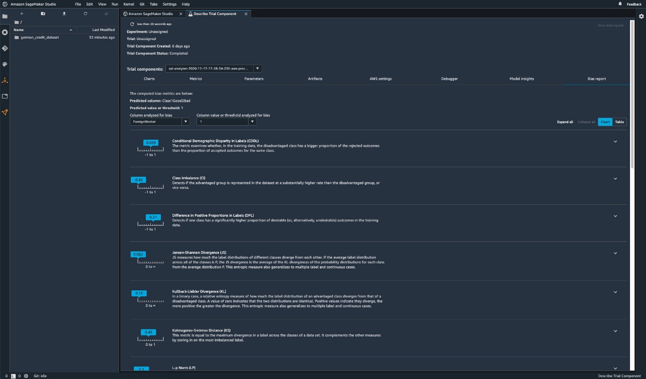
Questions about bias: Which metrics to start with?
Recall the sample questions about bias at the start of this post. Having gone through the metrics from different categories, consider the questions again. To answer the first question, which concerns the representations of different groups in the training data, you could start with the Class Imbalance (CI) metric. Similarly, for the remaining questions, you can start by looking into Difference in Positive Proportions in Labels (DPL), Accuracy Difference (AD), Difference in Acceptance Rate (DAR), and Recall Difference (RD), respectively.
Bias without facet values
For the ease of exposition, this description of posttraining metrics excluded the Generalized Entropy Index (GE) metric. This metric measures bias without considering the facet value, and can be helpful in assessing how the model errors are distributed. For details, refer to Generalized entropy (GE).
Conclusion
In this post, you saw how the 21 different metrics in SageMaker Clarify measure bias at different stages of the ML pipeline. You learned about various metrics via an income prediction use case, how to choose metrics for your use case, and which ones you could start with.
Get started with your responsible AI journey by assessing bias in your ML models by using the demo notebook Fairness and Explainability with SageMaker Clarify. You can find the detailed documentation for SageMaker Clarify, including the formal definition of metrics, at What Is Fairness and Model Explainability for Machine Learning Predictions. For the open-source implementation of the bias metrics, refer to the aws-sagemaker-clarify GitHub repository. For a detailed discussion including limitations, refer to Amazon AI Fairness and Explainability Whitepaper.
About the authors
 Bilal Zafar is an Applied Scientist at AWS, working on Fairness, Explainability and Security in Machine Learning.

Denis V. Batalov is a Solutions Architect for AWS, specializing in Machine Learning. He’s been with Amazon since 2005. Denis has a PhD in the field of AI. Follow him on Twitter: @dbatalov.
 Michele Donini is a Sr Applied Scientist at AWS. He leads a team of scientists working on Responsible AI and his research interests are Algorithmic Fairness and Explainable Machine Learning.