Posts in category: Amazon AWS

With personalized content more likely to drive customer engagement, businesses continuously seek to provide tailored content based on their customer’s profile and behavior. Recommendation systems in particular seek to predict the preference an end-user would give to an item. Some common use cases include product recommendations on online retail stores, personalizing newsletters, generating music playlist recommendations, or even discovering similar content on online media services.

However, it can be challenging to create an effective recommendation system due to complexities in model training, algorithm selection, and platform management. Amazon Personalize enables developers to improve customer engagement through personalized product and content recommendations with no machine learning (ML) expertise required. Developers can start to engage customers right away by using captured user behavior data. Behind the scenes, Amazon Personalize examines this data, identifies what is meaningful, selects the right algorithms, trains and optimizes a personalization model that is customized for your data, and provides recommendations via an API endpoint.

Although providing recommendations in real time can help boost engagement and satisfaction, sometimes this might not actually be required, and performing this in batch on a scheduled basis can simply be a more cost-effective and manageable option.

This post shows you how to use AWS services to not only create recommendations but also operationalize a batch recommendation pipeline. We walk through the end-to-end solution without a single line of code. We discuss two topics in detail:

• Preparing your data using AWS Glue
• Orchestrating the Amazon Personalize batch inference jobs using AWS Step Functions

Solution overview

In this solution, we use the MovieLens dataset. This dataset includes 86,000 ratings of movies from 2,113 users. We attempt to use this data to generate recommendations for each of these users.

Data preparation is very important to ensure we get customer behavior data into a format that is ready for Amazon Personalize. The architecture described in this post uses AWS Glue, a serverless data integration service, to perform the transformation of raw data into a format that is ready for Amazon Personalize to consume. The solution uses Amazon Personalize to create batch recommendations for all users by using a batch inference. We then use a Step Functions workflow so that the automated workflow can be run by calling Amazon Personalize APIs in a repeatable manner.

The following diagram demonstrates this solution.

We will build this solution with the following steps:

1. Build a data transformation job to transform our raw data using AWS Glue.
2. Build an Amazon Personalize solution with the transformed dataset.
3. Build a Step Functions workflow to orchestrate the generation of batch inferences.

Prerequisites

You need the following for this walkthrough:

• An AWS account
• Permissions to create new AWS Identity and Access Management (IAM) roles

Build a data transformation job to transform raw data with AWS Glue

With Amazon Personalize, input data needs to have a specific schema and file format. Data from interactions between users and items must be in CSV format with specific columns, whereas the list of users for which you want to generate recommendations for must be in JSON format. In this section, we use AWS Glue Studio to transform raw input data into the required structures and format for Amazon Personalize.

AWS Glue Studio provides a graphical interface that is designed for easy creation and running of extract, transform, and load (ETL) jobs. You can visually create data transformation workloads through simple drag-and-drop operations.

We first prepare our source data in Amazon Simple Storage Service (Amazon S3), then we transform the data without code.

1. On the Amazon S3 console, create an S3 bucket with three folders: raw, transformed, and curated.
2. Download the MovieLens dataset and upload the uncompressed file named user_ratingmovies-timestamp.dat to your bucket under the raw folder.
3. On the AWS Glue Studio console, choose Jobs in the navigation pane.
4. Select Visual with a source and target, then choose Create.
   
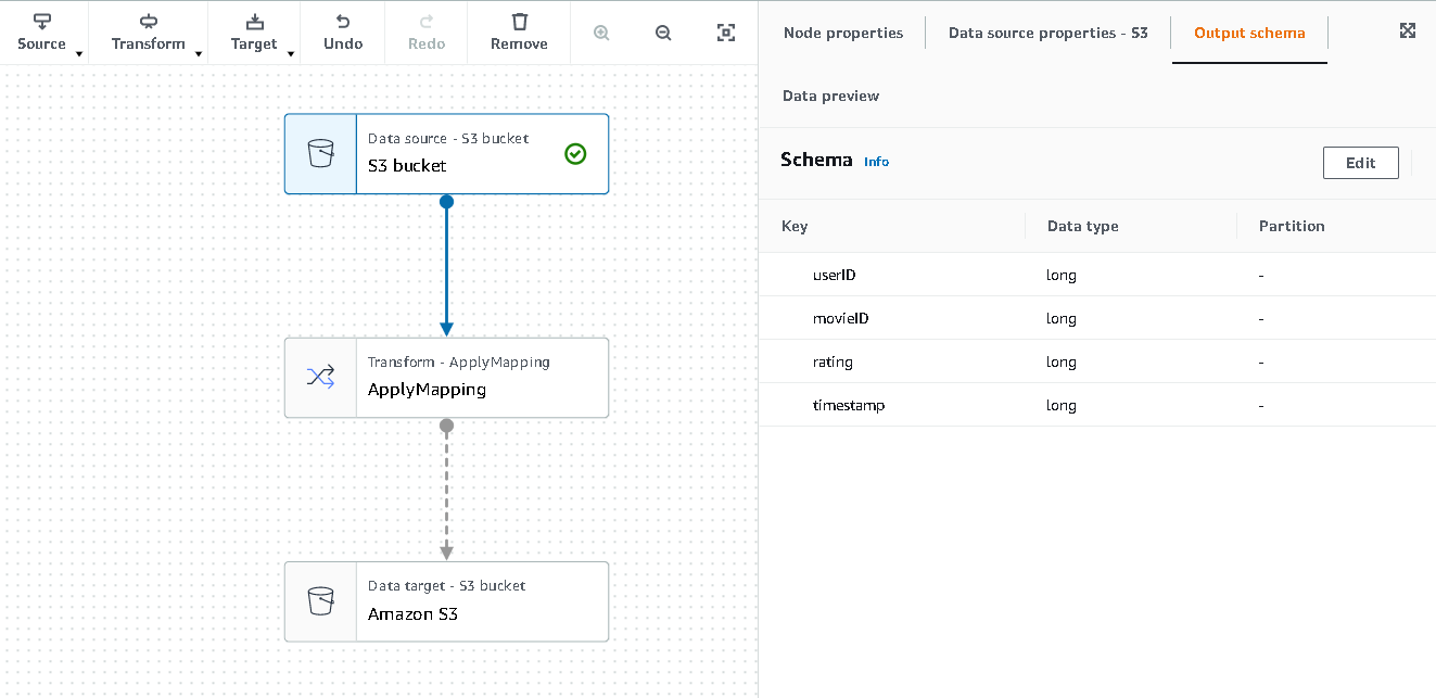
5. Choose the first node called Data source – S3 bucket. This is where we specify our input data.
6. On the Data source properties tab, select S3 location and browse to your uploaded file.
7. For Data format, choose CSV, and for Delimiter, choose Tab.
   
8. We can choose the Output schema tab to verify that the schema has inferred the columns correctly.
9. If the schema doesn’t match your expectations, choose Edit to edit the schema.
   

Next, we transform this data to follow the schema requirements for Amazon Personalize.

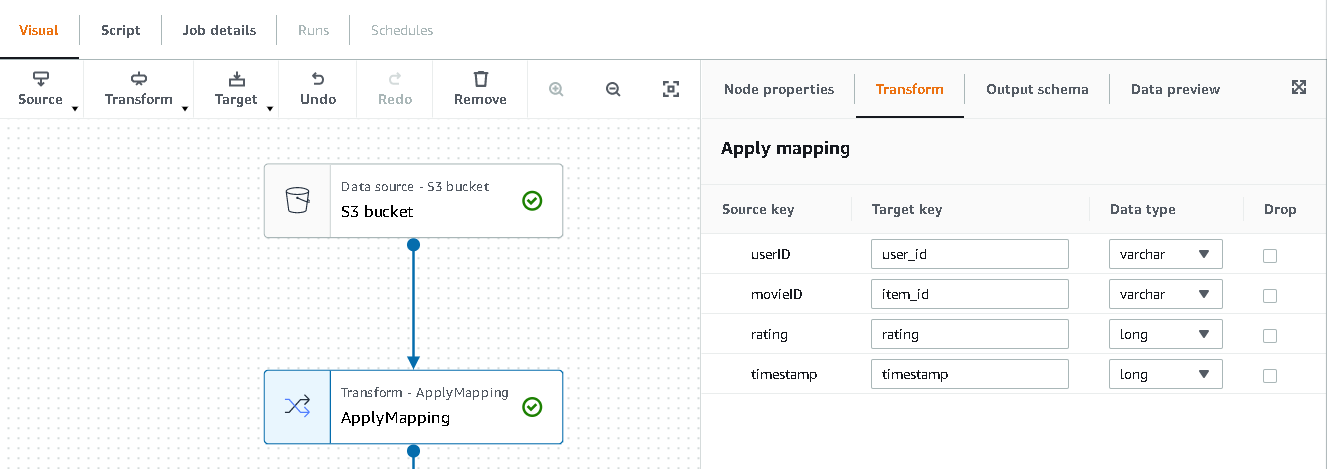
10. Choose the Transform – Apply Mapping node and, on the Transform tab, update the target key and data types.
    Amazon Personalize, at minimum, expects the following structure for the interactions dataset:

• • user_id (string)
  • item_id (string)
  • timestamp (long, in Unix epoch time format)
    

In this example, we exclude the poorly rated movies in the dataset.

11. To do so, remove the last node called S3 bucket and add a filter node on the Transform tab.
12. Choose Add condition and filter out data where rating < 3.5.
    

We now write the output back to Amazon S3.

13. Expand the Target menu and choose Amazon S3.
14. For S3 Target Location, choose the folder named transformed.
15. Choose CSV as the format and suffix the Target Location with interactions/.

Next, we output a list of users that we want to get recommendations for.

16. Choose the ApplyMapping node again, and then expand the Transform menu and choose ApplyMapping.
17. Drop all fields except for user_id and rename that field to userId. Amazon Personalize expects that field to be named userId.
18. Expand the Target menu again and choose Amazon S3.
19. This time, choose JSON as the format, and then choose the transformed S3 folder and suffix it with batch_users_input/.

This produces a JSON list of users as input for Amazon Personalize. We should now have a diagram that looks like the following.

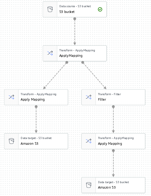
We are now ready to run our transform job.

20. On the IAM console, create a role called glue-service-role and attach the following managed policies:
    • AWSGlueServiceRole
    • AmazonS3FullAccess

For more information on how to create IAM service roles, refer to the Creating a role to delegate permissions to an AWS service.

21. Navigate back to your AWS Glue Studio job, and choose the Job details tab.
22. Set the job name as batch-personalize-input-transform-job.
23. Choose the newly created IAM role.
24. Keep the default values for everything else.
    
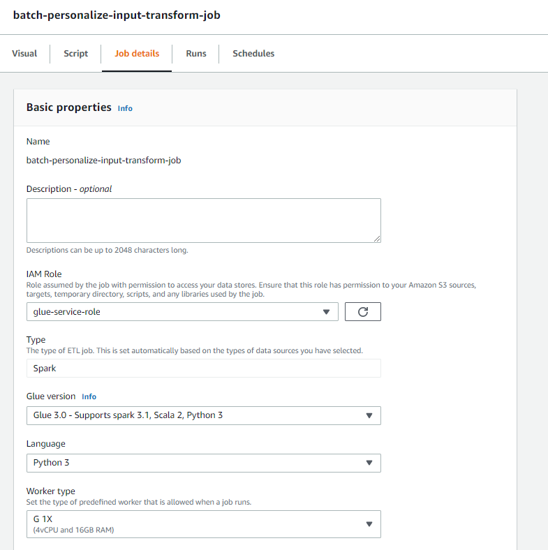
25. Choose Save.
26. When you’re ready, choose Run and monitor the job in the Runs tab.
27. When the job is complete, navigate to the Amazon S3 console to validate that your output file has been successfully created.

We have now shaped our data into the format and structure that Amazon Personalize requires. The transformed dataset should have the following fields and format:

• Interactions dataset – CSV format with fields USER_ID, ITEM_ID, TIMESTAMP
• User input dataset – JSON format with element userId

Build an Amazon Personalize solution with the transformed dataset

With our interactions dataset and user input data in the right format, we can now create our Amazon Personalize solution. In this section, we create our dataset group, import our data, and then create a batch inference job. A dataset group organizes resources into containers for Amazon Personalize components.

1. On the Amazon Personalize console, choose Create dataset group.
2. For Domain, select Custom.
3. Choose Create dataset group and continue.
   

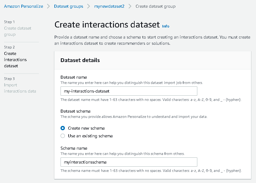
Next, create the interactions dataset.

4. Enter a dataset name and select Create new schema.
5. Choose Create dataset and continue.
   

We now import the interactions data that we had created earlier.

6. Navigate to the S3 bucket in which we created our interactions CSV dataset.
7. On the Permissions tab, add the following bucket access policy so that Amazon Personalize has access. Update the policy to include your bucket name.

   {
      "Version":"2012-10-17",
      "Id":"PersonalizeS3BucketAccessPolicy",
      "Statement":[
         {
            "Sid":"PersonalizeS3BucketAccessPolicy",
            "Effect":"Allow",
            "Principal":{
               "Service":"personalize.amazonaws.com"
            },
            "Action":[
               "s3:GetObject",
               "s3:ListBucket",
               "s3:PutObject"
            ],
            "Resource":[
               "arn:aws:s3:::<your-bucket-name>",
               "arn:aws:s3:::<your-bucket-name> /*"
            ]
         }
      ]
   }

Navigate back to Amazon Personalize and choose Create your dataset import job. Our interactions dataset should now be importing into Amazon Personalize. Wait for the import job to complete with a status of Active before continuing to the next step. This should take approximately 8 minutes.

8. On the Amazon Personalize console, choose Overview in the navigation pane and choose Create solution.
   
9. Enter a solution name.
10. For Solution type, choose Item recommendation.
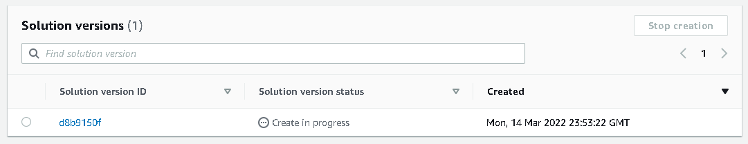
11. For Recipe, choose the aws-user-personalization recipe.
12. Choose Create and train solution.
    

The solution now trains against the interactions dataset that was imported with the user personalization recipe. Monitor the status of this process under Solution versions. Wait for it to complete before proceeding. This should take approximately 20 minutes.

We now create our batch inference job, which generates recommendations for each of the users present in the JSON input.

13. In the navigation pane, under Custom resources, choose Batch inference jobs.
14. Enter a job name, and for Solution, choose the solution created earlier.
15. Choose Create batch inference job.
    
16. For Input data configuration, enter the S3 path of where the batch_users_input file is located.

This is the JSON file that contains userId.

17. For Output data configuration path, choose the curated path in S3.
18. Choose Create batch inference job.

This process takes approximately 30 minutes. When the job is finished, recommendations for each of the users specified in the user input file are saved in the S3 output location.

We have successfully generated a set of recommendations for all of our users. However, we have only implemented the solution using the console so far. To make sure that this batch inferencing runs regularly with the latest set of data, we need to build an orchestration workflow. In the next section, we show you how to create an orchestration workflow using Step Functions.

Build a Step Functions workflow to orchestrate the batch inference workflow

To orchestrate your pipeline, complete the following steps:

1. On the Step Functions console, choose Create State Machine.
2. Select Design your workflow visually, then choose Next.
   
3. Drag the CreateDatasetImportJob node from the left (you can search for this node in the search box) onto the canvas.
4. Choose the node, and you should see the configuration API parameters on the right. Record the ARN.
5. Enter your own values in the API Parameters text box.

This calls the CreateDatasetImportJob API with the parameter values that you specify.

6. Drag the CreateSolutionVersion node onto the canvas.
7. Update the API parameters with the ARN of the solution that you noted down.

This creates a new solution version with the newly imported data by calling the CreateSolutionVersion API.

8. Drag the CreateBatchInferenceJob node onto the canvas and similarly update the API parameters with the relevant values.

Make sure that you use the $.SolutionVersionArn syntax to retrieve the solution version ARN parameter from the previous step. These API parameters are passed to the CreateBatchInferenceJob API.

We need to build a wait logic in the Step Functions workflow to make sure the recommendation batch inference job finishes before the workflow completes.

9. Find and drag in a Wait node.
10. In the configuration for Wait, enter 300 seconds.

This is an arbitrary value; you should alter this wait time according to your specific use case.

11. Choose the CreateBatchInferenceJob node again and navigate to the Error handling tab.
12. For Catch errors, enter Personalize.ResourceInUseException.
13. For Fallback state, choose Wait.

This step enables us to periodically check the status of the job and it only exits the loop when the job is complete.

14. For ResultPath, enter $.errorMessage.

This effectively means that when the “resource in use” exception is received, the job waits for x seconds before trying again with the same inputs.

15. Choose Save, and then choose Start the execution.

We have successfully orchestrated our batch recommendation pipeline for Amazon Personalize. As an optional step, you can use Amazon EventBridge to schedule a trigger of this workflow on a regular basis. For more details, refer to EventBridge (CloudWatch Events) for Step Functions execution status changes.

Clean up

To avoid incurring future charges, delete the resources that you created for this walkthrough.

Conclusion

In this post, we demonstrated how to create a batch recommendation pipeline by using a combination of AWS Glue, Amazon Personalize, and Step Functions, without needing a single line of code or ML experience. We used AWS Glue to prep our data into the format that Amazon Personalize requires. Then we used Amazon Personalize to import the data, create a solution with a user personalization recipe, and create a batch inferencing job that generates a default of 25 recommendations for each user, based on past interactions. We then orchestrated these steps using Step Functions so that we can run these jobs automatically.

For steps to consider next, user segmentation is one of the newer recipes in Amazon Personalize, which you might want to explore to create user segments for each row of the input data. For more details, refer to Getting batch recommendations and user segments.

About the author

Maxine Wee is an AWS Data Lab Solutions Architect. Maxine works with customers on their use cases, designs solutions to solve their business problems, and guides them through building scalable prototypes. Prior to her journey with AWS, Maxine helped customers implement BI, data warehousing, and data lake projects in Australia.

Read More

On August 9, 2022, we announced the general availability of cross-account sharing of Amazon SageMaker Pipelines entities. You can now use cross-account support for Amazon SageMaker Pipelines to share pipeline entities across AWS accounts and access shared pipelines directly through Amazon SageMaker API calls.

Customers are increasingly adopting multi-account architectures for deploying and managing machine learning (ML) workflows with SageMaker Pipelines. This involves building workflows in development or experimentation (dev) accounts, deploying and testing them in a testing or pre-production (test) account, and finally promoting them to production (prod) accounts to integrate with other business processes. You can benefit from cross-account sharing of SageMaker pipelines in the following use cases:

• When data scientists build ML workflows in a dev account, those workflows are then deployed by an ML engineer as a SageMaker pipeline into a dedicated test account. To further monitor those workflows, data scientists now require cross-account read-only permission to the deployed pipeline in the test account.
• ML engineers, ML admins, and compliance teams, who manage deployment and operations of those ML workflows from a shared services account, also require visibility into the deployed pipeline in the test account. They might also require additional permissions for starting, stopping, and retrying those ML workflows.

In this post, we present an example multi-account architecture for developing and deploying ML workflows with SageMaker Pipelines.

Solution overview

A multi-account strategy helps you achieve data, project, and team isolation while supporting software development lifecycle steps. Cross-account pipeline sharing supports a multi-account strategy, removing the overhead of logging in and out of multiple accounts and improving ML testing and deployment workflows by sharing resources directly across multiple accounts.

In this example, we have a data science team that uses a dedicated dev account for the initial development of the SageMaker pipeline. This pipeline is then handed over to an ML engineer, who creates a continuous integration and continuous delivery (CI/CD) pipeline in their shared services account to deploy this pipeline into a test account. To still be able to monitor and control the deployed pipeline from their respective dev and shared services accounts, resource shares are set up with AWS Resource Access Manager in the test and dev accounts. With this setup, the ML engineer and the data scientist can now monitor and control the pipelines in the dev and test accounts from their respective accounts, as shown in the following figure.

In the workflow, the data scientist and ML engineer perform the following steps:

1. The data scientist (DS) builds a model pipeline in the dev account.
2. The ML engineer (MLE) productionizes the model pipeline and creates a pipeline, (for this post, we call it sagemaker-pipeline).
3. sagemaker-pipeline code is committed to an AWS CodeCommit repository in the shared services account.
4. The data scientist creates an AWS RAM resource share for sagemaker-pipeline and shares it with the shared services account, which accepts the resource share.
5. From the shared services account, ML engineers are now able to describe, monitor, and administer the pipeline runs in the dev account using SageMaker API calls.
6. A CI/CD pipeline triggered in the shared service account builds and deploys the code to the test account using AWS CodePipeline.
7. The CI/CD pipeline creates and runs sagemaker-pipeline in the test account.
8. After running sagemaker-pipeline in the test account, the CI/CD pipeline creates a resource share for sagemaker-pipeline in the test account.
9. A resource share from the test sagemaker-pipeline with read-only permissions is created with the dev account, which accepts the resource share.
10. The data scientist is now able to describe and monitor the test pipeline run status using SageMaker API calls from the dev account.
11. A resource share from the test sagemaker-pipeline with extended permissions is created with the shared services account, which accepts the resource share.
12. The ML engineer is now able to describe, monitor, and administer the test pipeline run using SageMaker API calls from the shared services account.

In the following sections, we go into more detail and provide a demonstration on how to set up cross-account sharing for SageMaker pipelines.

How to create and share SageMaker pipelines across accounts

In this section, we walk through the necessary steps to create and share pipelines across accounts using AWS RAM and the SageMaker API.

Set up the environment

First, we need to set up a multi-account environment to demonstrate cross-account sharing of SageMaker pipelines:

1. Set up two AWS accounts (dev and test). You can set this up as member accounts of an organization or as independent accounts.
2. If you’re setting up your accounts as member of an organization, you can enable resource sharing with your organization. With this setting, when you share resources in your organization, AWS RAM doesn’t send invitations to principals. Principals in your organization gain access to shared resources without exchanging invitations.
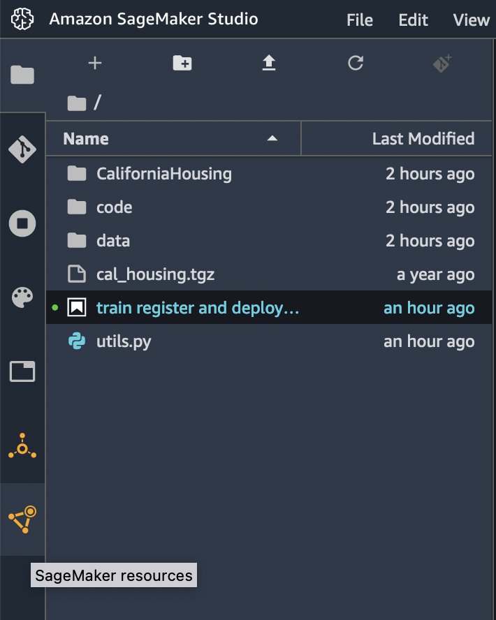
3. In the test account, launch Amazon SageMaker Studio and run the notebook train-register-deploy-pipeline-model. This creates an example pipeline in your test account. To simplify the demonstration, we use SageMaker Studio in the test account to launch the the pipeline. For real life projects, you should use Studio only in the dev account and launch SageMaker Pipeline in the test account using your CI/CD tooling.

Follow the instructions in the next section to share this pipeline with the dev account.

Set up a pipeline resource share

To share your pipeline with the dev account, complete the following steps:

1. On the AWS RAM console, choose Create resource share.
2. For Select resource type, choose SageMaker Pipelines.
3. Select the pipeline you created in the previous step.
4. Choose Next.
   
5. For Permissions, choose your associated permissions.
6. Choose Next.
   Next, you decide how you want to grant access to principals.
7. If you need to share the pipeline only within your organization accounts, select Allow Sharing only within your organization; otherwise select Allow sharing with anyone.
8. For Principals, choose your principal type (you can use an AWS account, organization, or organizational unit, based on your sharing requirement). For this post, we share with anyone at the AWS account level.
9. Select your principal ID.
10. Choose Next.
    
11. On the Review and create page, verify your information is correct and choose Create resource share.
    
12. Navigate to your destination account (for this post, your dev account).
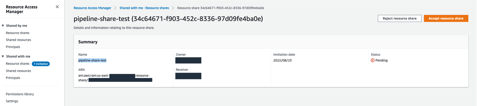
13. On the AWS RAM console, under Shared with me in the navigation pane, choose Resource shares.
14. Choose your resource share and choose Accept resource share.
    

Resource sharing permissions

When creating your resource share, you can choose from one of two supported permission policies to associate with the SageMaker pipeline resource type. Both policies grant access to any selected pipeline and all of its runs.

The AWSRAMDefaultPermissionSageMakerPipeline policy allows the following read-only actions:

"sagemaker:DescribePipeline"
"sagemaker:DescribePipelineDefinitionForExecution"
"sagemaker:DescribePipelineExecution"
"sagemaker:ListPipelineExecutions"
"sagemaker:ListPipelineExecutionSteps"
"sagemaker:ListPipelineParametersForExecution"
"sagemaker:Search"

The AWSRAMPermissionSageMakerPipelineAllowExecution policy includes all of the read-only permissions from the default policy, and also allows shared accounts to start, stop, and retry pipeline runs.

The extended pipeline run permission policy allows the following actions:

"sagemaker:DescribePipeline"
"sagemaker:DescribePipelineDefinitionForExecution"
"sagemaker:DescribePipelineExecution"
"sagemaker:ListPipelineExecutions"
"sagemaker:ListPipelineExecutionSteps"
"sagemaker:ListPipelineParametersForExecution"
"sagemaker:StartPipelineExecution"
"sagemaker:StopPipelineExecution"
"sagemaker:RetryPipelineExecution"
"sagemaker:Search"

Access shared pipeline entities through direct API calls

In this section, we walk through how you can use various SageMaker Pipeline API calls to gain visibility into pipelines running in remote accounts that have been shared with you. For testing the APIs against the pipeline running in the test account from the dev account, log in to the dev account and use AWS CloudShell.

For the cross-account SageMaker Pipeline API calls, you always need to use your pipeline ARN as the pipeline identification. That also includes the commands requiring the pipeline name, where you need to use your pipeline ARN as the pipeline name.

To get your pipeline ARN, in your test account, navigate to your pipeline details in Studio via SageMaker Resources.

Choose Pipelines on your resources list.

Choose your pipeline and go to your pipeline Settings tab. You can find the pipeline ARN with your Metadata information. For this example, your ARN is defined as "arn:aws:sagemaker:us-east-1:<account-id>:pipeline/serial-inference-pipeline".

ListPipelineExecutions

This API call lists the runs of your pipeline. Run the following command, replacing $SHARED_PIPELINE_ARN with your pipeline ARN from CloudShell or using the AWS Command Line Interface (AWS CLI) configured with the appropriated AWS Identity and Access Management (IAM) role:

aws sagemaker list-pipeline-executions --pipeline-name $SHARED_PIPELINE_ARN

The response lists all the runs of your pipeline with their PipelineExecutionArn, StartTime, PipelineExecutionStatus, and PipelineExecutionDisplayName:

{
  "PipelineExecutionSummaries": [
    {
      "PipelineExecutionArn": "arn:aws:sagemaker:<region>:<account_id>:pipeline/<pipeline_name>/execution/<execution_id>",
      "StartTime": "2022-08-10T11:32:05.543000+00:00",
      "PipelineExecutionStatus": "Executing",
      "PipelineExecutionDisplayName": "execution-321"
    },
    {
      "PipelineExecutionArn": "arn:aws:sagemaker:<region>:<account_id>:pipeline/<pipeline_name>/execution/<execution_id>",
      "StartTime": "2022-08-10T11:28:03.680000+00:00",
      "PipelineExecutionStatus": "Stopped",
      "PipelineExecutionDisplayName": "test"
    },
    {
      "PipelineExecutionArn": "arn:aws:sagemaker:<region>:<account_id>:pipeline/<pipeline_name>/execution/<execution_id>",
      "StartTime": "2022-08-10T11:03:47.406000+00:00",
      "PipelineExecutionStatus": "Succeeded",
      "PipelineExecutionDisplayName": "execution-123"
    }
  ]
}

DescribePipeline

This API call describes the detail of your pipeline. Run the following command, replacing $SHARED_PIPELINE_ARN with your pipeline ARN:

aws sagemaker describe-pipeline --pipeline-name $SHARED_PIPELINE_ARN

The response provides the metadata of your pipeline, as well as information about creation and modifications of it:

Output(truncated): 
{
"PipelineArn": "arn:aws:sagemaker:<region>:<account-id>:pipeline/<pipeline_name>",
"PipelineName": "serial-inference-pipeline",
"PipelineDisplayName": "serial-inference-pipeline",
"PipelineDefinition": "{"Version": "2020-12-01", "Metadata": {}, "Parameters": [{"Name": "TrainingInstanceType", "Type": "String", "DefaultValue": "ml.m5.xlarge"}, {"Name": "ProcessingInstanceType", "Type": "String", "DefaultValue": "ml.m5.xlarge"}, {"Name": "ProcessingInstanceCount", "Type": "Integer", "DefaultValue": 1}, {"Name": "InputData", "Type":

..

"PipelineStatus": "Active",
"CreationTime": "2022-08-08T21:33:39.159000+00:00",
"LastModifiedTime": "2022-08-08T21:48:14.274000+00:00",
"CreatedBy": {},
"LastModifiedBy": {}
}

DescribePipelineExecution

This API call describes the detail of your pipeline run. Run the following command, replacing $SHARED_PIPELINE_ARN with your pipeline ARN:

aws sagemaker describe-pipeline-execution 
--pipeline-execution-arn $PIPELINE_EXECUTION_ARN

The response provides details on your pipeline run, including the PipelineExecutionStatus, ExperimentName, and TrialName:

{
  "PipelineArn": "arn:aws:sagemaker:<region>:<account_id>:pipeline/<pipeline_name>",
  "PipelineExecutionArn": "arn:aws:sagemaker:<region>:<account_id>:pipeline/<pipeline_name>/execution/<execution_id>",
  "PipelineExecutionDisplayName": "execution-123",
  "PipelineExecutionStatus": "Succeeded",
  "PipelineExperimentConfig": {
  "ExperimentName": "<pipeline_name>",
  "TrialName": "<execution_id>"
},
  "CreationTime": "2022-08-10T11:03:47.406000+00:00",
  "LastModifiedTime": "2022-08-10T11:15:01.102000+00:00",
  "CreatedBy": {},
  "LastModifiedBy": {}
}

StartPipelineExecution

This API call starts a pipeline run. Run the following command, replacing $SHARED_PIPELINE_ARN with your pipeline ARN and $CLIENT_REQUEST_TOKEN with a unique, case-sensitive identifier that you generate for this run. The identifier should have between 32–128 characters. For instance, you can generate a string using the AWS CLI kms generate-random command.

aws sagemaker start-pipeline-execution 
  --pipeline-name $SHARED_PIPELINE_ARN 
  --client-request-token $CLIENT_REQUEST_TOKEN

As a response, this API call returns the PipelineExecutionArn of the started run:

{
  "PipelineExecutionArn": "arn:aws:sagemaker:<region>:<account_id>:pipeline/<pipeline_name>/execution/<execution_id>"
}

StopPipelineExecution

This API call stops a pipeline run. Run the following command, replacing $PIPELINE_EXECUTION_ARN with the pipeline run ARN of your running pipeline and $CLIENT_REQUEST_TOKEN with an unique, case-sensitive identifier that you generate for this run. The identifier should have between 32–128 characters. For instance, you can generate a string using the AWS CLI kms generate-random command.

aws sagemaker stop-pipeline-execution 
  --pipeline-execution-arn $PIPELINE_EXECUTION_ARN 
  --client-request-token $CLIENT_REQUEST_TOKEN

As a response, this API call returns the PipelineExecutionArn of the stopped pipeline:

{
  "PipelineExecutionArn": "arn:aws:sagemaker:<region>:<account_id>:pipeline/<pipeline_name>/execution/<execution_id>"
}

Conclusion

Cross-account sharing of SageMaker pipelines allows you to securely share pipeline entities across AWS accounts and access shared pipelines through direct API calls, without having to log in and out of multiple accounts.

In this post, we dove into the functionality to show how you can share pipelines across accounts and access them via SageMaker API calls.

As a next step, you can use this feature for your next ML project.

Resources

To get started with SageMaker Pipelines and sharing pipelines across accounts, refer to the following resources:

• Amazon SageMaker Model Building Pipelines
• Cross-Account Support for SageMaker Pipelines
• How resource sharing works

About the authors

Ram Vittal is an ML Specialist Solutions Architect at AWS. He has over 20 years of experience architecting and building distributed, hybrid, and cloud applications. He is passionate about building secure and scalable AI/ML and big data solutions to help enterprise customers with their cloud adoption and optimization journey to improve their business outcomes. In his spare time, he enjoys tennis, photography, and action movies.

Maira Ladeira Tanke is an ML Specialist Solutions Architect at AWS. With a background in data science, she has 9 years of experience architecting and building ML applications with customers across industries. As a technical lead, she helps customers accelerate their achievement of business value through emerging technologies and innovative solutions. In her free time, Maira enjoys traveling and spending time with her family someplace warm.

Gabriel Zylka is a Professional Services Consultant at AWS. He works closely with customers to accelerate their cloud adoption journey. Specialized in the MLOps domain, he focuses on productionizing machine learning workloads by automating end-to-end machine learning lifecycles and helping achieve desired business outcomes. In his spare time, he enjoys traveling and hiking in the Bavarian Alps.

Read More

Data preparation is the process of collecting, cleaning, and transforming raw data to make it suitable for insight extraction through machine learning (ML) and analytics. Data preparation is crucial for ML and analytics pipelines. Your model and insights will only be as reliable as the data you use for training them. Flawed data will produce poor results regardless of the sophistication of your algorithms and analytical tools.

Amazon SageMaker Data Wrangler is a service to help data scientists and data engineers simplify and accelerate tabular and time series data preparation and feature engineering through a visual interface. You can import data from multiple data sources, such as Amazon Simple Storage Service (Amazon S3), Amazon Athena, Amazon Redshift, Snowflake, and DataBricks, and process your data with over 300 built-in data transformations and a library of code snippets, so you can quickly normalize, transform, and combine features without writing any code. You can also bring your custom transformations in PySpark, SQL, or Pandas.

Previously, customers wanting to explore Data Wrangler needed to bring their own datasets; we’ve changed that. Starting today, you can begin experimenting with Data Wrangler’s features even faster by using a sample dataset and following suggested actions to easily navigate the product for the first time. In this post, we walk you through this process.

Solution overview

Data Wrangler offers a pre-loaded version of the well-known Titanic dataset, which is widely used to teach and experiment with ML. Data Wrangler’s suggested actions help first-time customers discover features such as Data Wrangler’s Data Quality and Insights Report, a feature that verifies data quality and helps detect abnormalities in your data.

In this post, we create a sample flow with the pre-loaded sample Titanic dataset to show how you can start experimenting with Data Wrangler’s features faster. We then use the processed Titanic dataset to create a classification model to tell us whether a passenger will survive or not, using the training functionality, which allows you to launch an Amazon SageMaker Autopilot experiment within any of the steps in a Data Wrangler flow. Along the way, we can explore Data Wrangler features through the product suggestions that surface in Data Wrangler. These suggestions can help you accelerate your learning curve with Data Wrangler by recommending actions and next steps.

Prerequisites

In order to get all the features described in this post, you need to be running the latest kernel version of Data Wrangler. For any new flow created, the kernel will always be the latest one; nevertheless, for existing flows, you need to update the Data Wrangler application first.

Import the Titanic dataset

The Titanic dataset is a public dataset widely used to teach and experiment with ML. You can use it to create an ML model that predicts which passengers will survive the Titanic shipwreck. Data Wrangler now incorporates this dataset as a sample dataset that you can use to get started with Data Wrangler more quickly. In this post, we perform some data transformations using this dataset.

Let’s create a new Data Wrangler flow and call it Titanic. Data Wrangler shows you two options: you can either import your own dataset or you can use the sample dataset (the Titanic dataset).

You’re presented with a loading bar that indicates the progress of the dataset being imported into Data Wrangler. Click through the carousel to learn more about how Data Wrangler helps you import, prepare, and process datasets for ML. Wait until the bar is fully loaded; this indicates that your dataset is imported and ready for use.

The Titanic dataset is now loaded into our flow. For a description of the dataset, refer to Titanic – Machine Learning from Disaster.

Explore Data Wrangler features

As a first-time Data Wrangler user, you now see suggested actions to help you navigate the product and discover interesting features. Let’s follow the suggested advice.

1. Choose the plus sign to get a list of options to modify the dataset.
   
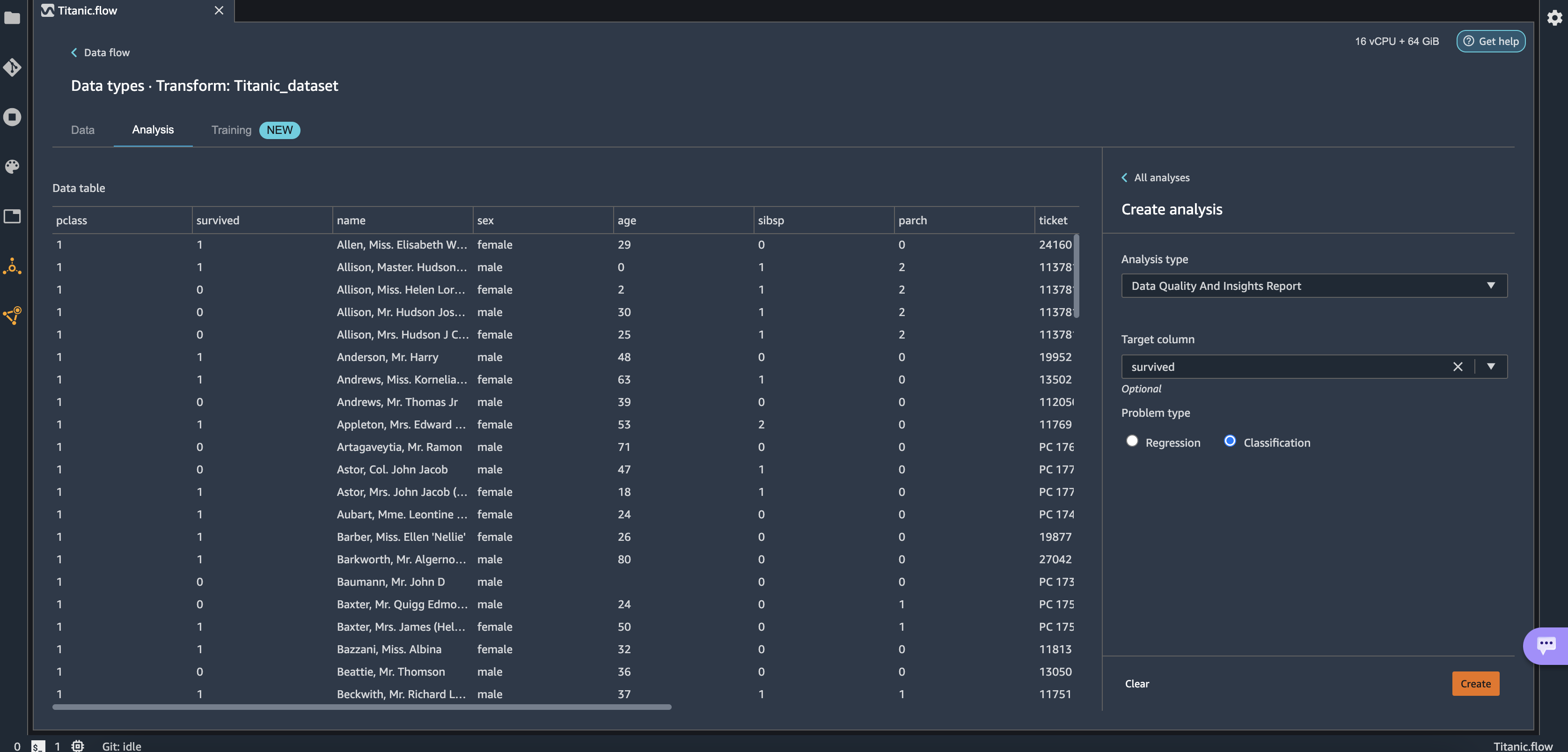
2. Choose Get data insights.
   
   This opens the Analysis tab on the data, in which you can create a Data Quality and Insights Report. When you create this report, Data Wrangler gives you the option to select a target column. A target column is a column that you’re trying to predict. When you choose a target column, Data Wrangler automatically creates a target column analysis. It also ranks the features in the order of their predictive power. When you select a target column, you must specify whether you’re trying to solve a regression or a classification problem.
3. Choose the column survived as the target column because that’s the value we want to predict.
4. For Problem type¸ select Classification¸ because we want to know whether a passenger belongs to the survived or not survived classes.
5. Choose Create.
   This creates an analysis on your dataset that contains relevant points like a summary of the dataset, duplicate rows, anomalous samples, feature details, and more. To learn more about the Data Quality and Insights Report, refer to Accelerate data preparation with data quality and insights in Amazon SageMaker Data Wrangler and Get Insights On Data and Data Quality.
   Let’s get a quick look at the dataset itself.
6. Choose the Data tab to visualize the data as a table.Let’s now generate some example data visualizations.
7. Choose the Analysis tab to start visualizing your data. You can generate three histograms: the first two visualize the number of people that survived based on the sex and class columns, as shown in the following screenshots.The third visualizes the ages of the people that boarded the Titanic.Let’s perform some transformations on the data,
8. First, drop the columns ticket, cabin, and name.
9. Next, perform one-hot encoding on the categorical columns embarked and sex, and home.dest.
10. Finally, fill in missing values for the columns boat and body with a 0 value.
    Your dataset now looks something like the following screenshot.
11. Now split the dataset into three sets: a training set with 70% of the data, a validation set with 20% of the data, and a test set with 10% of the data.The splits done here use the stratified split approach using the survived variable and are just for the sake of the demonstration.Now let’s configure the destination of our data.
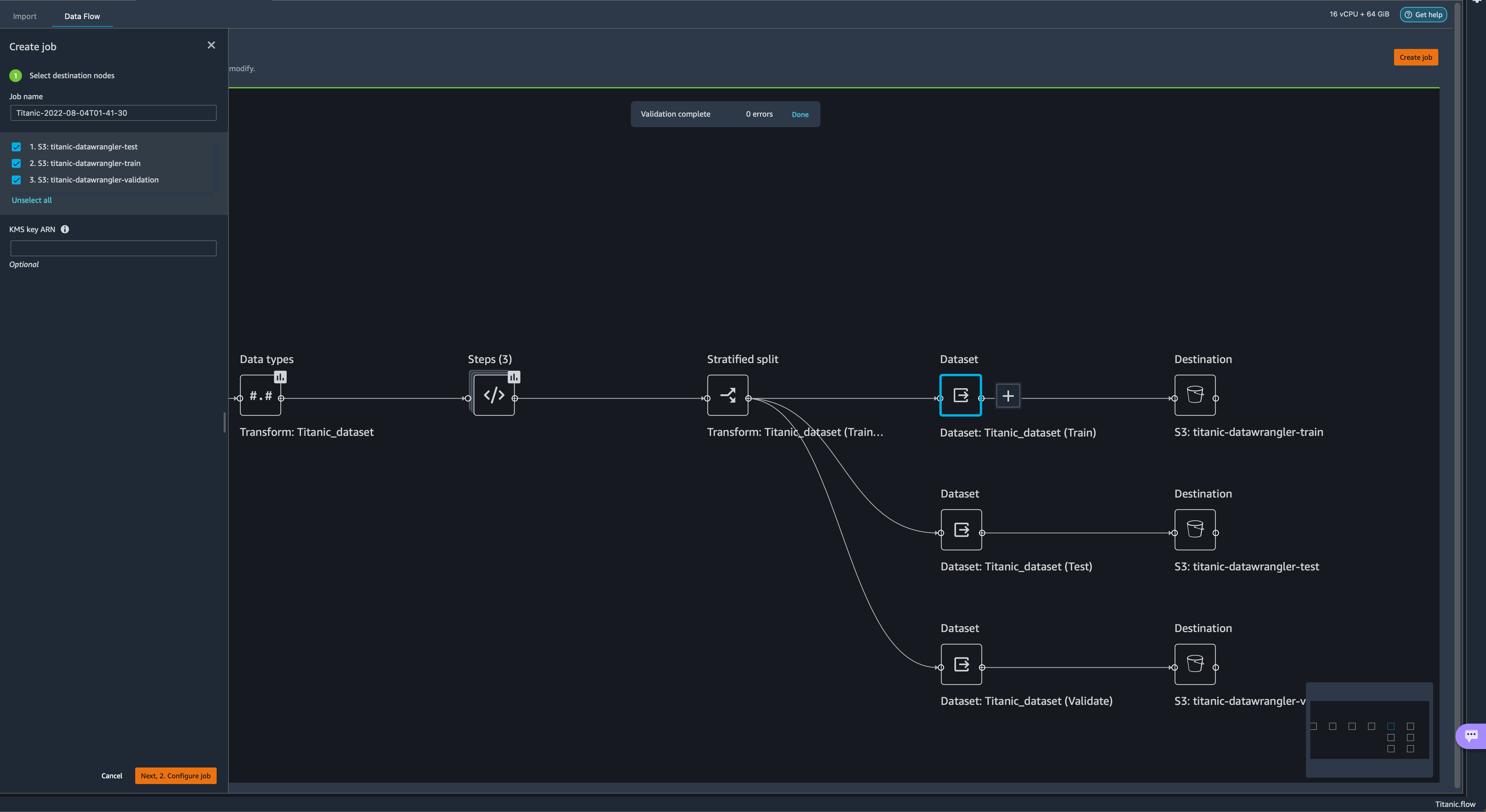
12. Choose the plus sign on each Dataset node, choose Add destination, and choose S3 to add an Amazon S3 destination for the transformed datasets.
13. In the Add a destination pane, you can configure the Amazon S3 details to store your processed datasets.Our Titanic flow should now look like the following screenshot.You can now transform all the data using SageMaker processing jobs.
14. Choose Create job.
15. Keep the default values and choose Next.
16. Choose Run.A new SageMaker processing job is now created. You can see the job’s details and track its progress on the SageMaker console under Processing jobs.When the processing job is complete, you can navigate to any of the S3 locations specified for storing the datasets and query the data just to confirm that the processing was successful. You can now use this data to feed your ML projects.

Launch an Autopilot experiment to create a classifier

You can now launch Autopilot experiments directly from Data Wrangler and use the data at any of the steps in the flow to automatically train a model on the data.

1. Choose the Dataset node called Titanic_dataset (train) and navigate to the Train tab.
   Before training, you need to first export your data to Amazon S3.
2. Follow the instructions to export your data to an S3 location of your choice.
   You can specify to export the data in CSV or Parquet format for increased efficiency. Additionally, you can specify an AWS Key Management Service (AWS KMS) key to encrypt your data.
   On the next page, you configure your Autopilot experiment.
3. Unless your data is split into several parts, leave the default value under Connect your data.
4. For this demonstration, leave the default values for Experiment name and Output data location.
5. Under Advanced settings, expand Machine learning problem type.
6. Choose Binary classification as the problem type and Accuracy as the objective metric.You specify these two values manually even though Autopilot is capable of inferring them from the data.
7. Leave the rest of the fields with the default values and choose Create Experiment.Wait for a couple of minutes until the Autopilot experiment is complete, and you will see a leaderboard like the following with each of the models obtained by Autopilot.

You can now choose to deploy any of the models in the leaderboard for inference.

Clean up

When you’re not using Data Wrangler, it’s important to shut down the instance on which it runs to avoid incurring additional fees.

To avoid losing work, save your data flow before shutting Data Wrangler down.

1. To save your data flow in Amazon SageMaker Studio, choose File, then choose Save Data Wrangler Flow.
   Data Wrangler automatically saves your data flow every 60 seconds.
2. To shut down the Data Wrangler instance, in Studio, choose Running Instances and Kernels.
3. Under RUNNING APPS, choose the shutdown icon next to the sagemaker-data-wrangler-1.0 app.
4. Choose Shut down all to confirm.Data Wrangler runs on an ml.m5.4xlarge instance. This instance disappears from RUNNING INSTANCES when you shut down the Data Wrangler app.

After you shut down the Data Wrangler app, it has to restart the next time you open a Data Wrangler flow file. This can take a few minutes.

Conclusion

In this post, we demonstrated how you can use the new sample dataset on Data Wrangler to explore Data Wrangler’s features without needing to bring your own data. We also presented two additional features: the loading page to let you visually track the progress of the data being imported into Data Wrangler, and product suggestions that provide useful tips to get started with Data Wrangler. We went further to show how you can create SageMaker processing jobs and launch Autopilot experiments directly from the Data Wrangler user interface.

To learn more about using data flows with Data Wrangler, refer to Create and Use a Data Wrangler Flow and Amazon SageMaker Pricing. To get started with Data Wrangler, see Prepare ML Data with Amazon SageMaker Data Wrangler. To learn more about Autopilot and AutoML on SageMaker, visit Automate model development with Amazon SageMaker Autopilot.

About the authors

David Laredo is a Prototyping Architect at AWS Envision Engineering in LATAM, where he has helped develop multiple machine learning prototypes. Previously, he worked as a Machine Learning Engineer and has been doing machine learning for over 5 years. His areas of interest are NLP, time series, and end-to-end ML.

Parth Patel is a Solutions Architect at AWS in the San Francisco Bay Area. Parth guides customers to accelerate their journey to the cloud and helps them adopt the AWS Cloud successfully. He focuses on ML and application modernization.

Read More

In December 2020, AWS announced the general availability of Amazon SageMaker JumpStart, a capability of Amazon SageMaker that helps you quickly and easily get started with machine learning (ML). JumpStart provides one-click fine-tuning and deployment of a wide variety of pre-trained models across popular ML tasks, as well as a selection of end-to-end solutions that solve common business problems. These features remove the heavy lifting from each step of the ML process, making it easier to develop high-quality models and reducing time to deployment.

This post is the third in a series on using JumpStart for specific ML tasks. In the first post, we showed how you can run image classification use cases on JumpStart. In the second post, we showed how you can run text classification use cases on JumpStart. In this post, we provide a step-by-step walkthrough on how to fine-tune and deploy an image segmentation model, using trained models from MXNet. We explore two ways of obtaining the same result: via JumpStart’s graphical interface on Amazon SageMaker Studio, and programmatically through JumpStart APIs.

If you want to jump straight into the JumpStart API code we explain in this post, you can refer to the following sample Jupyter notebooks:

• Introduction to JumpStart – Instance Segmentation
• Introduction to JumpStart – Semantic Segmentation

JumpStart overview

JumpStart helps you get started with ML models for a variety of tasks without writing a single line of code. At the time of writing, JumpStart enables you to do the following:

• Deploy pre-trained models for common ML tasks – JumpStart enables you to address common ML tasks with no development effort by providing easy deployment of models pre-trained on large, publicly available datasets. The ML research community has put a large amount of effort into making a majority of recently developed models publicly available for use. JumpStart hosts a collection of over 300 models, spanning the 15 most popular ML tasks such as object detection, text classification, and text generation, making it easy for beginners to use them. These models are drawn from popular model hubs such as TensorFlow, PyTorch, Hugging Face, and MXNet.
• Fine-tune pre-trained models – JumpStart allows you to fine-tune pre-trained models with no need to write your own training algorithm. In ML, the ability to transfer the knowledge learned in one domain to another domain is called transfer learning. You can use transfer learning to produce accurate models on your smaller datasets, with much lower training costs than the ones involved in training the original model. JumpStart also includes popular training algorithms based on LightGBM, CatBoost, XGBoost, and Scikit-learn, which you can train from scratch for tabular regression and classification.
• Use pre-built solutions – JumpStart provides a set of 17 solutions for common ML use cases, such as demand forecasting and industrial and financial applications, which you can deploy with just a few clicks. Solutions are end-to-end ML applications that string together various AWS services to solve a particular business use case. They use AWS CloudFormation templates and reference architectures for quick deployment, which means they’re fully customizable.
• Refer to notebook examples for SageMaker algorithms – SageMaker provides a suite of built-in algorithms to help data scientists and ML practitioners get started with training and deploying ML models quickly. JumpStart provides sample notebooks that you can use to quickly use these algorithms.
• Review training videos and blogs – JumpStart also provides numerous blog posts and videos that teach you how to use different functionalities within SageMaker.

JumpStart accepts custom VPC settings and AWS Key Management Service (AWS KMS) encryption keys, so you can use the available models and solutions securely within your enterprise environment. You can pass your security settings to JumpStart within Studio or through the SageMaker Python SDK.

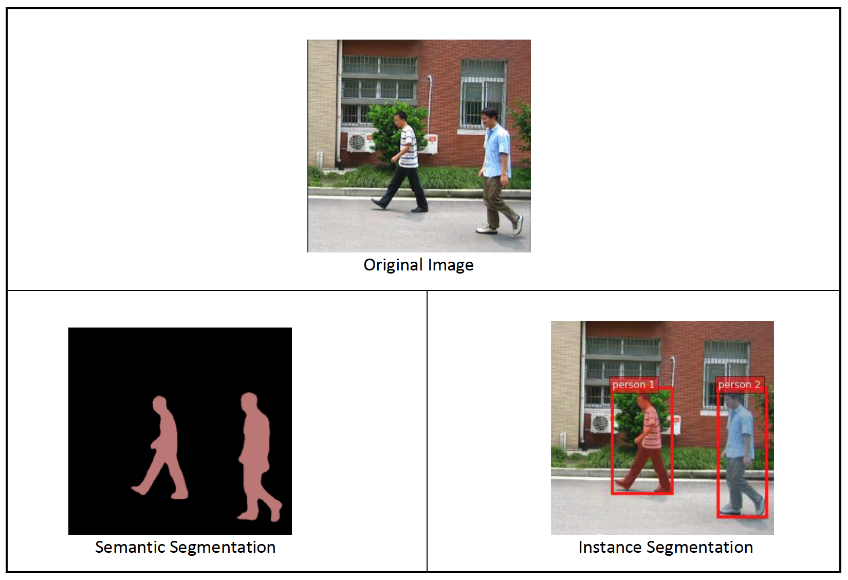
Semantic segmentation

Semantic segmentation delineates each class of objects appearing in an input image. It tags (classifies) each pixel of the input image with a class label from a predefined set of classes. Multiple objects of the same class are mapped to the same mask.

The model available for fine-tuning builds a fully convolutional network (FCN) “head” on top of the base network. The fine-tuning step fine-tunes the FCNHead while keeping the parameters of the rest of the model frozen, and returns the fine-tuned model. The objective is to minimize per-pixel softmax cross entropy loss to train the FCN. The model returned by fine-tuning can be further deployed for inference.

The input directory should look like the following code if the training data contains two images. The names of the .png files can be anything.

input_directory
    |--images
        |--abc.png
        |--def.png
    |--masks
        |--abc.png
        |--def.png
    class_label_to_prediction_index.json

The mask files should have class label information for each pixel.

Instance segmentation

Instance segmentation detects and delineates each distinct object of interest appearing in an image. It tags every pixel with an instance label. Whereas semantic segmentation assigns the same tag to pixels of multiple objects of the same class, instance segmentation further labels pixels corresponding to each occurrence of an object on the image with a separate tag.

Currently, JumpStart offers inference-only models for instance segmentation and doesn’t support fine-tuning.

The following images illustrate the difference between the inference in semantic segmentation and instance segmentation. The original image has two people in the image. Semantic segmentation treats multiple people in the image as one entity: Person. However, instance segmentation identifies individual people within the Person category.

Solution overview

The following sections provide a step-by-step demo to perform semantic segmentation with JumpStart, both via the Studio UI and via JumpStart APIs.

We walk through the following steps:

1. Access JumpStart through the Studio UI:
   1. Run inference on the pre-trained model.
   2. Fine-tune the pre-trained model.
2. Use JumpStart programmatically with the SageMaker Python SDK:
   1. Run inference on the pre-trained model.
   2. Fine-tune the pre-trained model.

We also discuss additional advanced features of JumpStart.

Access JumpStart through the Studio UI

In this section, we demonstrate how to train and deploy JumpStart models through the Studio UI.

Run inference on the pre-trained model

The following video shows you how to find a pre-trained semantic segmentation model on JumpStart and deploy it. The model page contains valuable information about the model, how to use it, expected data format, and some fine-tuning details. You can deploy any of the pre-trained models available in JumpStart. For inference, we pick the ml.g4dn.xlarge instance type. It provides the GPU acceleration needed for low inference latency, but at a lower price point. After you configure the SageMaker hosting instance, choose Deploy. It may take 5–10 minutes until your persistent endpoint is up and running.

After a few minutes, your endpoint is operational and ready to respond to inference requests.

Similarly, you can deploy a pre-trained instance segmentation model by following the same steps in the preceding video while searching for instance segmentation instead of semantic segmentation in the JumpStart search bar.

Fine-tune the pre-trained model

The following video shows how to find and fine-tune a semantic segmentation model in JumpStart. In the video, we fine-tune the model using the PennFudanPed dataset, provided by default in JumpStart, which you can download under the Apache 2.0 License.

Fine-tuning on your own dataset involves taking the correct formatting of data (as explained on the model page), uploading it to Amazon Simple Storage Service (Amazon S3), and specifying its location in the data source configuration. We use the same hyperparameter values set by default (number of epochs, learning rate, and batch size). We also use a GPU-backed ml.p3.2xlarge as our SageMaker training instance.

You can monitor your training job running directly on the Studio console, and are notified upon its completion. After training is complete, you can deploy the fine-tuned model from the same page that holds the training job details. The deployment workflow is the same as deploying a pre-trained model.

Use JumpStart programmatically with the SageMaker SDK

In the preceding sections, we showed how you can use the JumpStart UI to deploy a pre-trained model and fine-tune it interactively, in a matter of a few clicks. However, you can also use JumpStart’s models and easy fine-tuning programmatically by using APIs that are integrated into the SageMaker SDK. We now go over a quick example of how you can replicate the preceding process. All the steps in this demo are available in the accompanying notebooks Introduction to JumpStart – Instance Segmentation and Introduction to JumpStart – Semantic Segmentation.

Run inference on the pre-trained model

In this section, we choose an appropriate pre-trained model in JumpStart, deploy this model to a SageMaker endpoint, and run inference on the deployed endpoint.

SageMaker is a platform based on Docker containers. JumpStart uses the available framework-specific SageMaker Deep Learning Containers (DLCs). We fetch any additional packages, as well as scripts to handle training and inference for the selected task. Finally, the pre-trained model artifacts are separately fetched with model_uris, which provides flexibility to the platform. You can use any number of models pre-trained for the same task with a single training or inference script. See the following code:

model_id, model_version = "mxnet-semseg-fcn-resnet50-ade", "*"

# Retrieve the inference docker container uri
deploy_image_uri = image_uris.retrieve(
    region=None,
    framework=None,  # automatically inferred from model_id
    image_scope="inference",
    model_id=model_id,
    model_version=model_version,
    instance_type=inference_instance_type,
)

# Retrieve the inference script uri
deploy_source_uri = script_uris.retrieve(model_id=model_id, model_version=model_version, script_scope="inference")

base_model_uri = model_uris.retrieve(model_id=model_id, model_version=model_version, model_scope="inference")

For instance segmentation, we can set model_id to mxnet-semseg-fcn-resnet50-ade. The is in the identifier corresponds to instance segmentation.

Next, we feed the resources into a SageMaker model instance and deploy an endpoint:

# Create the SageMaker model instance
model = Model(
    image_uri=deploy_image_uri,
    source_dir=deploy_source_uri,
    model_data=base_model_uri,
    entry_point="inference.py",  # entry point file in source_dir and present in deploy_source_uri
    role=aws_role,
    predictor_cls=Predictor,
    name=endpoint_name,
)

# deploy the Model. Note that we need to pass Predictor class when we deploy model through Model class,
# for being able to run inference through the sagemaker API.
base_model_predictor = model.deploy(
    initial_instance_count=1,
    instance_type=inference_instance_type,
    predictor_cls=Predictor,
    endpoint_name=endpoint_name,
)

After a few minutes, our model is deployed and we can get predictions from it in real time!

The following code snippet gives you a glimpse of what semantic segmentation looks like. The predicted mask for each pixel is visualized. To get inferences from a deployed model, an input image needs to be supplied in binary format. The response of the endpoint is a predicted label for each pixel in the image. We use the query_endpoint and parse_response helper functions, which are defined in the accompanying notebook:

query_response = query(base_model_predictor, pedestrian_img)
predictions, labels, image_labels = parse_response(query_response)
print("Objects present in the picture:", image_labels)

Fine-tune the pre-trained model

To fine-tune a selected model, we need to get that model’s URI, as well as that of the training script and the container image used for training. Thankfully, these three inputs depend solely on the model name, version (for a list of the available models, see JumpStart Available Model Table), and the type of instance you want to train on. This is demonstrated in the following code snippet:

from sagemaker import image_uris, model_uris, script_uris

model_id, model_version = "mxnet-semseg-fcn-resnet50-ade", "*"
training_instance_type = "ml.p3.2xlarge"
train_image_uri = image_uris.retrieve(
    region=None,
    framework=None,
    model_id=model_id,
    model_version=model_version,
    image_scope="training",
    instance_type=training_instance_type,)# Retrieve the training script

train_source_uri = script_uris.retrieve(model_id=model_id, model_version=model_version, script_scope="training")# Retrieve the pre-trained model tarball to further fine-tune

train_model_uri = model_uris.retrieve(model_id=model_id, model_version=model_version, model_scope="training")

We retrieve the model_id corresponding to the same model we used previously. You can now fine-tune this JumpStart model on your own custom dataset using the SageMaker SDK. We use a dataset that is publicly hosted on Amazon S3, conveniently focused on semantic segmentation. The dataset should be structured for fine-tuning as explained in the previous section. See the following example code:

# URI of your training dataset
training_data_bucket = f"jumpstart-cache-prod-{aws_region}"
training_data_prefix = "training-datasets/PennFudanPed_SemSeg/"
training_dataset_s3_path = f"s3://{training_data_bucket}/{training_data_prefix}"
training_job_name = name_from_base(f"jumpstart-example-{model_id}-transfer-learning")# Create SageMaker Estimator instance
semseg_estimator = Estimator(
    role=aws_role,
    image_uri=train_image_uri,
    source_dir=train_source_uri,
    model_uri=train_model_uri,
    entry_point="transfer_learning.py",
    instance_count=1,
    instance_type=training_instance_type,
    max_run=360000,
    hyperparameters=hyperparameters,
    output_path=s3_output_location,)# Launch a SageMaker Training job by passing s3 path of the training data
semseg_estimator.fit({"training": training_dataset_s3_path}, logs=True)

We obtain the same default hyperparameters for our selected model as the ones we saw in the previous section, using sagemaker.hyperparameters.retrieve_default(). We then instantiate a SageMaker estimator and call the .fit method to start fine-tuning our model, passing it the Amazon S3 URI for our training data. The entry_point script provided is named transfer_learning.py (the same for other tasks and models), and the input data channel passed to .fit must be named training.

While the algorithm trains, you can monitor its progress either in the SageMaker notebook where you’re running the code itself, or on Amazon CloudWatch. When training is complete, the fine-tuned model artifacts are uploaded to the Amazon S3 output location specified in the training configuration. You can now deploy the model in the same manner as the pre-trained model.

Advanced features

In addition to fine-tuning and deploying pre-trained models, JumpStart offers many advanced features.

The first is automatic model tuning. This allows you to automatically tune your ML models to find the hyperparameter values with the highest accuracy within the range provided through the SageMaker API.

The second is incremental training. This allows you to train a model you have already fine-tuned using an expanded dataset that contains an underlying pattern not accounted for in previous fine-tuning runs, which resulted in poor model performance. Incremental training saves both time and resources because you don’t need to retrain the model from scratch.

Conclusion

In this post, we showed how to fine-tune and deploy a pre-trained semantic segmentation model, and how to adapt it for instance segmentation using JumpStart. You can accomplish this without needing to write code. Try out the solution on your own and send us your comments.

To learn more about JumpStart and how you can use open-source pre-trained models for a variety of other ML tasks, check out the following AWS re:Invent 2020 video.

About the Authors

Dr. Vivek Madan is an Applied Scientist with the Amazon SageMaker JumpStart team. He got his PhD from University of Illinois at Urbana-Champaign and was a Post Doctoral Researcher at Georgia Tech. He is an active researcher in machine learning and algorithm design and has published papers in EMNLP, ICLR, COLT, FOCS, and SODA conferences.

Santosh Kulkarni is an Enterprise Solutions Architect at Amazon Web Services who works with sports customers in Australia. He is passionate about building large-scale distributed applications to solve business problems using his knowledge in AI/ML, big data, and software development.

Leonardo Bachega is a senior scientist and manager in the Amazon SageMaker JumpStart team. He’s passionate about building AI services for computer vision.

Read More

Organizations in the lending and mortgage industry process thousands of documents on a daily basis. From a new mortgage application to mortgage refinance, these business processes involve hundreds of documents per application. There is limited automation available today to process and extract information from all the documents, especially due to varying formats and layouts. Due to high volume of applications, capturing strategic insights and getting key information from the contents is a time-consuming, highly manual, error prone and expensive process. Legacy optical character recognition (OCR) tools are cost-prohibitive, error-prone, involve a lot of configuring, and are difficult to scale. Intelligent document processing (IDP) with AWS artificial intelligence (AI) services helps automate and accelerate the mortgage application processing with goals of faster and quality decisions, while reducing overall costs.

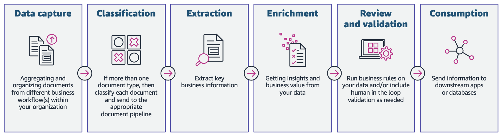
In this post, we demonstrate how you can utilize machine learning (ML) capabilities with Amazon Textract, and Amazon Comprehend to process documents in a new mortgage application, without the need for ML skills. We explore the various phases of IDP as shown in the following figure, and how they connect to the steps involved in a mortgage application process, such as application submission, underwriting, verification, and closing.

Although each mortgage application may be unique, we took into account some of the most common documents that are included in a mortgage application, such as the Unified Residential Loan Application (URLA-1003) form, 1099 forms, and mortgage note.

Solution overview

Amazon Textract is an ML service that automatically extracts text, handwriting, and data from scanned documents using pre-trained ML models. Amazon Comprehend is a natural-language processing (NLP) service that uses ML to uncover valuable insights and connections in text and can perform document classification, name entity recognition (NER), topic modeling, and more.

The following figure shows the phases of IDP as it relates to the phases of a mortgage application process.

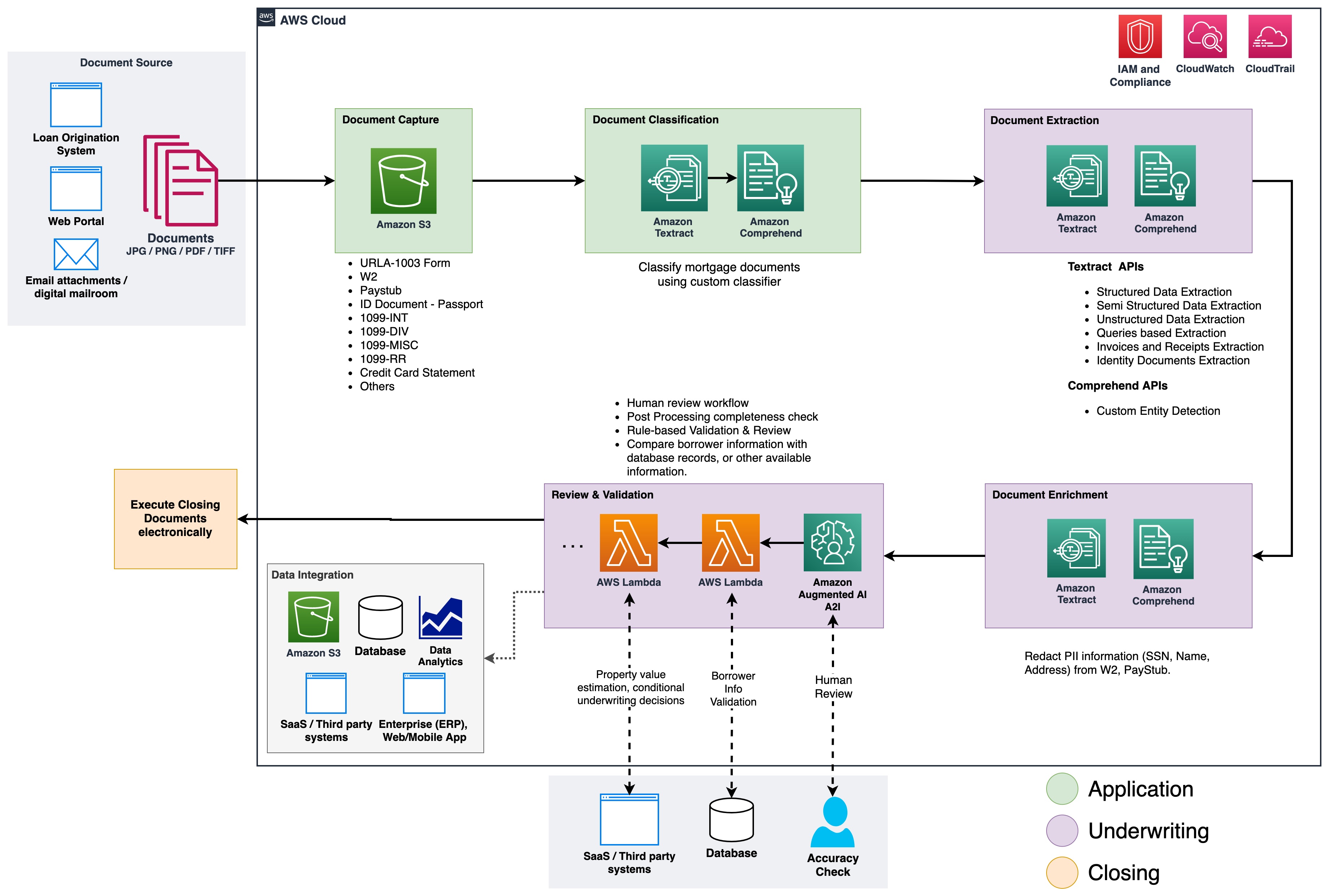
At the start of the process, documents are uploaded to an Amazon Simple Storage Service (Amazon S3) bucket. This initiates a document classification process to categorize the documents into known categories. After the documents are categorized, the next step is to extract key information from them. We then perform enrichment for select documents, which can be things like personally identifiable information (PII) redaction, document tagging, metadata updates, and more. The next step involves validating the data extracted in previous phases to ensure completeness of a mortgage application. Validation can be done via business validation rules and cross document validation rules. The confidence scores of the extracted information can also be compared to a set threshold, and automatically routed to a human reviewer through Amazon Augmented AI (Amazon A2I) if the threshold isn’t met. In the final phase of the process, the extracted and validated data is sent to downstream systems for further storage, processing, or data analytics.

In the following sections, we discuss the phases of IDP as it relates to the phases of a mortgage application in detail. We walk through the phases of IDP and discuss the types of documents; how we store, classify, and extract information, and how we enrich the documents using machine learning.

Document storage

Amazon S3 is an object storage service that offers industry-leading scalability, data availability, security, and performance. We use Amazon S3 to securely store the mortgage documents during and after the mortgage application process. A mortgage application packet may contain several types of forms and documents, such as URLA-1003, 1099-INT/DIV/RR/MISC, W2, paystubs, bank statements, credit card statements, and more. These documents are submitted by the applicant in the mortgage application phase. Without manually looking through them, it might not be immediately clear which documents are included in the packet. This manual process can be time-consuming and expensive. In the next phase, we automate this process using Amazon Comprehend to classify the documents into their respective categories with high accuracy.

Document classification

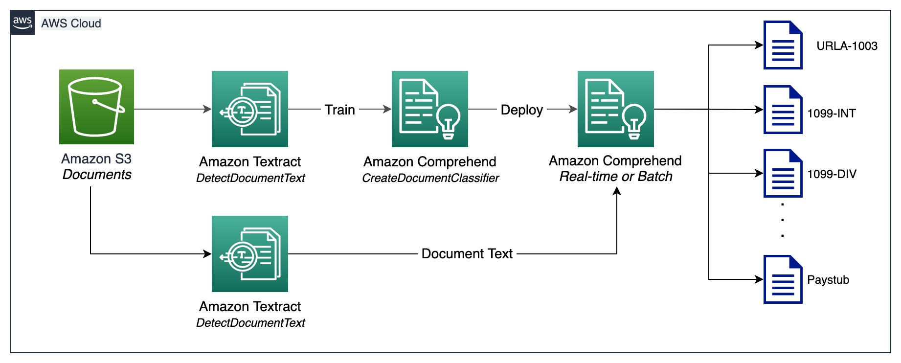
Document classification is a method by means of which a large number of unidentified documents can be categorized and labeled. We perform this document classification using an Amazon Comprehend custom classifier. A custom classifier is an ML model that can be trained with a set of labeled documents to recognize the classes that are of interest to you. After the model is trained and deployed behind a hosted endpoint, we can utilize the classifier to determine the category (or class) a particular document belongs to. In this case, we train a custom classifier in multi-class mode, which can be done either with a CSV file or an augmented manifest file. For the purposes of this demonstration, we use a CSV file to train the classifier. Refer to our GitHub repository for the full code sample. The following is a high-level overview of the steps involved:

1. Extract UTF-8 encoded plain text from image or PDF files using the Amazon Textract DetectDocumentText API.
2. Prepare training data to train a custom classifier in CSV format.
3. Train a custom classifier using the CSV file.
4. Deploy the trained model with an endpoint for real-time document classification or use multi-class mode, which supports both real-time and asynchronous operations.

The following diagram illustrates this process.

You can automate document classification using the deployed endpoint to identify and categorize documents. This automation is useful to verify whether all the required documents are present in a mortgage packet. A missing document can be quickly identified, without manual intervention, and notified to the applicant much earlier in the process.

Document extraction

In this phase, we extract data from the document using Amazon Textract and Amazon Comprehend. For structured and semi-structured documents containing forms and tables, we use the Amazon Textract AnalyzeDocument API. For specialized documents such as ID documents, Amazon Textract provides the AnalyzeID API. Some documents may also contain dense text, and you may need to extract business-specific key terms from them, also known as entities. We use the custom entity recognition capability of Amazon Comprehend to train a custom entity recognizer, which can identify such entities from the dense text.

In the following sections, we walk through the sample documents that are present in a mortgage application packet, and discuss the methods used to extract information from them. For each of these examples, a code snippet and a short sample output is included.

Extract data from Unified Residential Loan Application URLA-1003

A Unified Residential Loan Application (URLA-1003) is an industry standard mortgage loan application form. It’s a fairly complex document that contains information about the mortgage applicant, type of property being purchased, amount being financed, and other details about the nature of the property purchase. The following is a sample URLA-1003, and our intention is to extract information from this structured document. Because this is a form, we use the AnalyzeDocument API with a feature type of FORM.

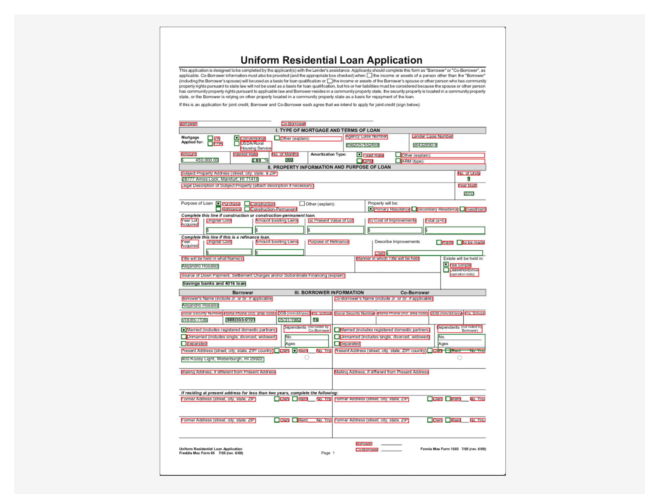
The FORM feature type extracts form information from the document, which is then returned in key-value pair format. The following code snippet uses the amazon-textract-textractor Python library to extract form information with just a few lines of code. The convenience method call_textract() calls the AnalyzeDocument API internally, and the parameters passed to the method abstract some of the configurations that the API needs to run the extraction task. Document is a convenience method used to help parse the JSON response from the API. It provides a high-level abstraction and makes the API output iterable and easy to get information out of. For more information, refer to Textract Response Parser and Textractor.

from textractcaller.t_call import call_textract, Textract_Features
from trp import Document

response_urla_1003 = call_textract(input_document='s3://<your-bucket>/URLA-1003.pdf', 
                                   features=[Textract_Features.FORMS])
doc_urla_1003 = Document(response_urla_1003)
for page in doc_urla_1003.pages:
    forms=[]
    for field in page.form.fields:
        obj={}
        obj[f'{field.key}']=f'{field.value}'
        forms.append(obj)
print(json.dumps(forms, indent=4))

Note that the output contains values for check boxes or radio buttons that exist in the form. For example, in the sample URLA-1003 document, the Purchase option was selected. The corresponding output for the radio button is extracted as “Purchase” (key) and “SELECTED” (value), indicating that radio button was selected.

[
    { "No. of Units": "1" },
    { "Amount": "$ 450,000.00" },
    { "Year Built": "2010" },
    { "Purchase": "SELECTED" },
    { "Title will be held in what Name(s)": "Alejandro Rosalez" },
    { "Fixed Rate": "SELECTED" },
    ...
]

Extract data from 1099 forms

A mortgage application packet may also contain a number of IRS documents, such as 1099-DIV, 1099-INT, 1099-MISC, and 1099-R. These documents show the applicant’s earnings via interests, dividends, and other miscellaneous income components that are useful during underwriting to make decisions. The following image shows a collection of these documents, which are similar in structure. However, in some instances, the documents contain form information (marked using the red and green bounding boxes) as well as tabular information (marked by the yellow bounding boxes).

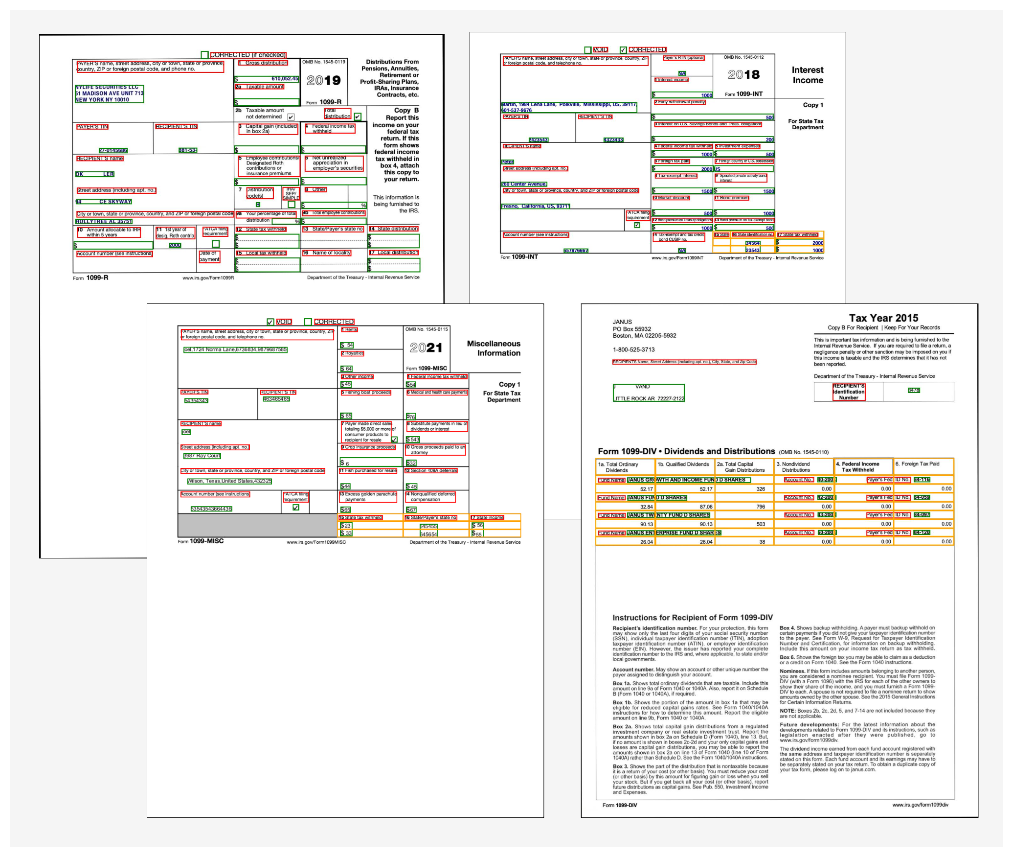
To extract form information, we use similar code as explained earlier with the AnalyzeDocument API. We pass an additional feature of TABLE to the API to indicate that we need both form and table data extracted from the document. The following code snippet uses the AnalyzeDocument API with FORMS and TABLES features on the 1099-INT document:

from textractcaller.t_call import call_textract, Textract_Features
from trp import Document
response_1099_int = call_textract(input_document='s3://<your-bucket>/1099-INT-2018.pdf',
                                  features=[Textract_Features.TABLES, 
                                            Textract_Features.FORMS])
doc_1099_int = Document(response_1099_int)
num_tables=1
for page in doc_1099_int.pages:     
    for table in page.tables:
        num_tables=num_tables+1
        for r, row in enumerate(table.rows):
            for c, cell in enumerate(row.cells):
                print(f"Cell[{r}][{c}] = {cell.text}")
        print('n')

Because the document contains a single table, the output of the code is as follows:

Table 1
-------------------
Cell[0][0] = 15 State 
Cell[0][1] = 16 State identification no. 
Cell[0][2] = 17 State tax withheld 
Cell[1][0] = 
Cell[1][1] = 34564 
Cell[1][2] = $ 2000 
Cell[2][0] = 
Cell[2][1] = 23543 
Cell[2][2] = $ 1000

The table information contains the cell position (row 0, column 0, and so on) and the corresponding text within each cell. We use a convenience method that can transform this table data into easy-to-read grid view:

from textractprettyprinter.t_pretty_print import Textract_Pretty_Print, get_string, Pretty_Print_Table_Format
print(get_string(textract_json=response_1099_int, 
                 table_format=Pretty_Print_Table_Format.grid, 
                 output_type=[Textract_Pretty_Print.TABLES]))

We get the following output:

+----------+-----------------------------+-----------------------+
| 15 State | 16 State identification no. | 17 State tax withheld |
+----------+-----------------------------+-----------------------+
|          | 34564                       | $ 2000                |
+----------+-----------------------------+-----------------------+
|          | 23543                       | $ 1000                |
+----------+-----------------------------+-----------------------+

To get the output in an easy-to-consume CSV format, the format type of Pretty_Print_Table_Format.csv can be passed into the table_format parameter. Other formats such as TSV (tab separated values), HTML, and Latex are also supported. For more information, refer to Textract-PrettyPrinter.

Extract data from a mortgage note

A mortgage application packet may contain unstructured documents with dense text. Some examples of dense text documents are contracts and agreements. A mortgage note is an agreement between a mortgage applicant and the lender or mortgage company, and contains information in dense text paragraphs. In such cases, the lack of structure makes it difficult to find key business information that is important in the mortgage application process. There are two approaches to solving this problem:

• Use the Amazon Textract AnalyzeDocument API with the Queries feature
• Use an Amazon Comprehend custom entity recognizer

In the following sample mortgage note, we’re specifically interested in finding out the monthly payment amount and principal amount.

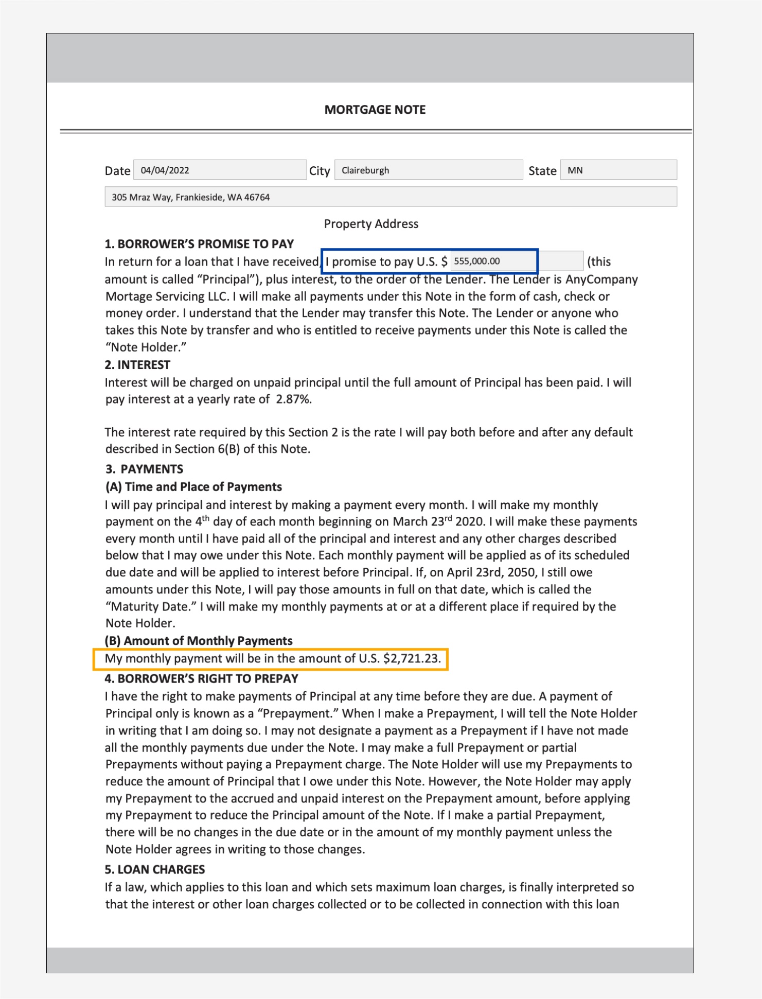
For the first approach, we use the Query and QueriesConfig convenience methods to configure a set of questions that is passed to the Amazon Textract AnalyzeDocument API call. In case the document is multi-page (PDF or TIFF), we can also specify the page numbers where Amazon Textract should look for answers to the question. The following code snippet demonstrates how to create the query configuration, make an API call, and subsequently parse the response to get the answers from the response:

from textractcaller import QueriesConfig, Query
import trp.trp2 as t2

#Setup the queries
query2 = Query(text="What is the principal amount borrower has to pay?", alias="PRINCIPAL_AMOUNT", pages=["1"])
query4 = Query(text="What is the monthly payment amount?", alias="MONTHLY_AMOUNT", pages=["1"])

#Setup the query config with the above queries
queries_config = QueriesConfig(queries=[query1, query2, query3, query4])
#Call AnalyzeDocument with the queries_config
response_mortgage_note = call_textract(input_document='s3://<your-bucket>/Mortgage-Note.pdf',
                                       features=[Textract_Features.QUERIES],
                                       queries_config=queries_config)
doc_mortgage_note: t2.TDocumentSchema = t2.TDocumentSchema().load(response_mortgage_note) 

entities = {}
for page in doc_mortgage_note.pages:
    query_answers = doc_mortgage_note.get_query_answers(page=page)
    if query_answers:
        for answer in query_answers:
            entities[answer[1]] = answer[2]
print(entities)

We get the following output:

{
    'PRINCIPAL_AMOUNT': '$ 555,000.00',
    'MONTHLY_AMOUNT': '$2,721.23',
}

For the second approach, we use the Amazon Comprehend DetectEntities API with the mortgage note, which returns the entities it detects within the text from a predefined set of entities. These are entities that the Amazon Comprehend entity recognizer is pre-trained with. However, because our requirement is to detect specific entities, an Amazon Comprehend custom entity recognizer is trained with a set of sample mortgage note documents, and a list of entities. We define the entity names as PRINCIPAL_AMOUNT and MONTHLY_AMOUNT. Training data is prepared following the Amazon Comprehend training data preparation guidelines for custom entity recognition. The entity recognizer can be trained with document annotations or with entity lists. For the purposes of this example, we use entity lists to train the model. After we train the model, we can deploy it with a real-time endpoint or in batch mode to detect the two entities from the document contents. The following are the steps involved to train a custom entity recognizer and deploy it. For a full code walkthrough, refer to our GitHub repository.

1. Prepare the training data (the entity list and the documents with (UTF-8 encoded) plain text format).
2. Start the entity recognizer training using the CreateEntityRecognizer API using the training data.
3. Deploy the trained model with a real-time endpoint using the CreateEndpoint API.

Extract data from a US passport

The Amazon Textract analyze identity documents capability can detect and extract information from US-based ID documents such as a driver’s license and passport. The AnalyzeID API is capable of detecting and interpreting implied fields in ID documents, which makes it easy to extract specific information from the document. Identity documents are almost always part of a mortgage application packet, because it’s used to verify the identity of the borrower during the underwriting process, and to validate the correctness of the borrower’s biographical data.

We use a convenience method named call_textract_analyzeid, which calls the AnalyzeID API internally. We then iterate over the response to obtain the detected key-value pairs from the ID document. See the following code:

from textractcaller import call_textract_analyzeid
import trp.trp2_analyzeid as t2id

response_passport = call_textract_analyzeid(document_pages=['s3://<your-bucket>/Passport.pdf'])
doc_passport: t2id.TAnalyzeIdDocument = t2id.TAnalyzeIdDocumentSchema().load(response_passport)

for id_docs in response_passport['IdentityDocuments']:
    id_doc_kvs={}
    for field in id_docs['IdentityDocumentFields']:
        if field['ValueDetection']['Text']:
            id_doc_kvs[field['Type']['Text']] = field['ValueDetection']['Text']
print(id_doc_kvs)

AnalyzeID returns information in a structure called IdentityDocumentFields, which contains the normalized keys and their corresponding value. For example, in the following output, FIRST_NAME is a normalized key and the value is ALEJANDRO. In the example passport image, the field for the first name is labeled as “Given Names / Prénoms / Nombre,” however AnalyzeID was able to normalize that into the key name FIRST_NAME. For a list of supported normalized fields, refer to Identity Documentation Response Objects.

{
    'FIRST_NAME': 'ALEJANDRO',
    'LAST_NAME': 'ROSALEZ',
    'DOCUMENT_NUMBER': '918268822',
    'EXPIRATION_DATE': '31 JAN 2029',
    'DATE_OF_BIRTH': '15 APR 1990',
    'DATE_OF_ISSUE': '29 JAN 2009',
    'ID_TYPE': 'PASSPORT',
    'ENDORSEMENTS': 'SEE PAGE 27',
    'PLACE_OF_BIRTH': 'TEXAS U.S.A.'
}

A mortgage packet may contain several other documents, such as a paystub, W2 form, bank statement, credit card statement, and employment verification letter. We have samples for each of these documents along with the code required to extract data from them. For the complete code base, check out the notebooks in our GitHub repository.

Document enrichment

One of the most common forms of document enrichment is sensitive or confidential information redaction on documents, which may be mandated due to privacy laws or regulations. For example, a mortgage applicant’s paystub may contain sensitive PII data, such as name, address, and SSN, that may need redaction for extended storage.

In the preceding sample paystub document, we perform redaction of PII data such as SSN, name, bank account number, and dates. To identify PII data in a document, we use the Amazon Comprehend PII detection capability via the DetectPIIEntities API. This API inspects the content of the document to identify the presence of PII information. Because this API requires input in UTF-8 encoded plain text format, we first extract the text from the document using the Amazon Textract DetectDocumentText API, which returns the text from the document and also returns geometry information such as bounding box dimensions and coordinates. A combination of both outputs is then used to draw redactions on the document as part of the enrichment process.

Review, validate, and integrate data

Extracted data from the document extraction phase may need validation against specific business rules. Specific information may also be validated across several documents, also known as cross-doc validation. An example of cross-doc validation could be comparing the applicant’s name in the ID document to the name in the mortgage application document. You can also do other validations such as property value estimations and conditional underwriting decisions in this phase.

A third type of validation is related to the confidence score of the extracted data in the document extraction phase. Amazon Textract and Amazon Comprehend return a confidence score for forms, tables, text data, and entities detected. You can configure a confidence score threshold to ensure that only correct values are being sent downstream. This is achieved via Amazon A2I, which compares the confidence scores of detected data with a predefined confidence threshold. If the threshold isn’t met, the document and the extracted output is routed to a human for review through an intuitive UI. The reviewer takes corrective action on the data and saves it for further processing. For more information, refer to Core Concepts of Amazon A2I.

Conclusion

In this post, we discussed the phases of intelligent document processing as it relates to phases of a mortgage application. We looked at a few common examples of documents that can be found in a mortgage application packet. We also discussed ways of extracting and processing structured, semi-structured, and unstructured content from these documents. IDP provides a way to automate end-to-end mortgage document processing that can be scaled to millions of documents, enhancing the quality of application decisions, reducing costs, and serving customers faster.

As a next step, you can try out the code samples and notebooks in our GitHub repository. To learn more about how IDP can help your document processing workloads, visit Automate data processing from documents.

About the authors

Anjan Biswas is a Senior AI Services Solutions Architect with focus on AI/ML and Data Analytics. Anjan is part of the world-wide AI services team and works with customers to help them understand, and develop solutions to business problems with AI and ML. Anjan has over 14 years of experience working with global supply chain, manufacturing, and retail organizations and is actively helping customers get started and scale on AWS AI services.

Dwiti Pathak is a Senior Technical Account Manager based out of San Diego. She is focused on helping Semiconductor industry engage in AWS. In her spare time, she likes reading about new technologies and playing board games.

Balaji Puli is a Solutions Architect based in Bay Area, CA. Currently helping select Northwest U.S healthcare life sciences customers accelerate their AWS cloud adoption. Balaji enjoys traveling and loves to explore different cuisines.

Read More