Posts in category: Amazon AWS

So much data, so little time. Machine learning (ML) experts, data scientists, engineers and enthusiasts have encountered this problem the world over. From natural language processing to computer vision, tabular to time series, and everything in-between, the age-old problem of optimizing for speed when running data against as many GPUs as you can get has inspired countless solutions. Today, we’re happy to announce features for PyTorch developers using native open-source frameworks, like PyTorch Lightning and PyTorch DDP, that will streamline their path to the cloud.

Amazon SageMaker is a fully-managed service for ML, and SageMaker model training is an optimized compute environment for high-performance training at scale. SageMaker model training offers a remote training experience with a seamless control plane to easily train and reproduce ML models at high performance and low cost. We’re thrilled to announce new features in the SageMaker training portfolio that make running PyTorch at scale even easier and more accessible:

1. PyTorch Lightning can now be integrated to SageMaker’s distributed data parallel library with only one-line of code change.
2. SageMaker model training now has support for native PyTorch Distributed Data Parallel with NCCL backend, allowing developers to migrate onto SageMaker easier than ever before.

In this post, we discuss these new features, and also learn how Amazon Search has run PyTorch Lightning with the optimized distributed training backend in SageMaker to speed up model training time.

Before diving into the Amazon Search case study, for those who aren’t familiar we would like to give some background on SageMaker’s distributed data parallel library. In 2020, we developed and launched a custom cluster configuration for distributed gradient descent at scale that increases overall cluster efficiency, introduced on Amazon Science as Herring. Using the best of both parameter servers and ring-based topologies, SageMaker Distributed Data Parallel (SMDDP) is optimized for the Amazon Elastic Compute Cloud (Amazon EC2) network topology, including EFA. For larger cluster sizes, SMDDP is able to deliver 20–40% throughput improvements relative to Horovod (TensorFlow) and PyTorch Distributed Data Parallel. For smaller cluster sizes and supported models, we recommend the SageMaker Training Compiler, which is able to decrease overall job time by up to 50%.

Customer spotlight: PyTorch Lightning on SageMaker’s optimized backend with Amazon Search

Amazon Search is responsible for the search and discovery experience on Amazon.com. It powers the search experience for customers looking for products to buy on Amazon. At a high level, Amazon Search builds an index for all products sold on Amazon.com. When a customer enters a query, Amazon Search then uses a variety of ML techniques, including deep learning models, to match relevant and interesting products to the customer query. Then it ranks the products before showing the results to the customer.

Amazon Search scientists have used PyTorch Lightning as one of the main frameworks to train the deep learning models that power Search ranking due to its added usability features on top of PyTorch. SMDDP was not supported for deep learning models written in PyTorch Lightning before this new SageMaker launch. This prevented Amazon Search scientists who prefer using PyTorch Lightning from scaling their model training using data parallel techniques, significantly slowing down their training time and preventing them from testing new experiments that require more scalable training.

The team’s early benchmarking results show 7.3 times faster training time for a sample model when trained on eight nodes as compared to a single-node training baseline. The baseline model used in these benchmarking is a multi-layer perceptron neural network with seven dense fully connected layers and over 200 parameters. The following table summarizes the benchmarking result on ml.p3.16xlarge SageMaker training instances.

Next, we dive into the details on the new launches. If you like, you can step through our corresponding example notebook .

Run PyTorch Lightning with the SageMaker distributed training library

We are happy to announce that SageMaker Data Parallel now seamlessly integrates with PyTorch Lightning within SageMaker training.

PyTorch Lightning is an open-source framework that provides a simplification for writing custom models in PyTorch. In some ways similar to what Keras did for TensorFlow, or even arguably Hugging Face, PyTorch Lightning provides a high-level API with abstractions for much of the lower-level functionality of PyTorch itself. This includes defining the model, profiling, evaluation, pruning, model parallelism, hyperparameter configurations, transfer learning, and more.

Previously, PyTorch Lightning developers were uncertain about how to seamlessly migrate their training code on to high-performance SageMaker GPU clusters. In addition, there was no way for them to take advantage of efficiency gains introduced by SageMaker Data Parallel.

For PyTorch Lightning, generally speaking, there should be little-to-no code changes to simply run these APIs on SageMaker Training. In the example notebooks we use the DDPStrategy and DDPPlugin methods.

There are three steps to use PyTorch Lightning with SageMaker Data Parallel as an optimized backend:

1. Use a supported AWS Deep Learning Container (DLC) as your base image, or optionally create your own container and install the SageMaker Data Parallel backend yourself. Ensure that you have PyTorch Lightning included in your necessary packages, such as with a requirements.txt file.
2. Make a few minor code changes to your training script that enable the optimized backend. These include:
   1. Import the SM DDP library:

      import smdistributed.dataparallel.torch.torch_smddp
      

   2. Set up the PyTorch Lightning environment for SageMaker:

      from pytorch_lightning.plugins.environments.lightning_environment 
        import LightningEnvironment
      
      env = LightningEnvironment()
      env.world_size = lambda: int(os.environ["WORLD_SIZE"])
      env.global_rank = lambda: int(os.environ["RANK"])

   3. If you’re using a version of PyTorch Lightning older than 1.5.10, you’ll need to add a few more steps.
      1. First, add the environment variable:

         os.environ["PL_TORCH_DISTRIBUTED_BACKEND"] = "smddp"

      2. Second, ensure you use DDPPlugin, rather than DDPStrategy. If you’re using a more recent version, which you can easily set by placing the requirements.txt in the source_dir for your job, then this isn’t necessary. See the following code:

         ddp = DDPPlugin(parallel_devices=[torch.device("cuda", d) for d in range(num_gpus)], cluster_environment=env)

   4. Optionally, define your process group backend as "smddp" in the DDPSTrategy object. However, if you’re using PyTorch Lightning with the PyTorch DDP backend, which is also supported, simply remove this `process_group_backend` parameter. See the following code:

      ddp = DDPStrategy(
        cluster_environment=env, 
        process_group_backend="smddp", 
        accelerator="gpu")

3. Ensure that you have a distribution method noted in the estimator, such as distribution={"smdistributed":{"dataparallel":{"enabled":True} if you’re using the Herring backend, or distribution={"pytorchddp":{"enabled":True}.

• For a full listing of suitable parameters in the distribution parameter, see our documentation here.

Now you can launch your SageMaker training job! You can launch your training job via the Python SDK, Boto3, the SageMaker console, the AWS Command Line Interface (AWS CLI), and countless other methods. From an AWS perspective, this is a single API command: create-training-job. Whether you launch this command from your local terminal, an AWS Lambda function, an Amazon SageMaker Studio notebook, a KubeFlow pipeline, or any other compute environment is completely up to you.

Please note that the integration between PyTorch Lightning and SageMaker Data Parallel is currently supported for only newer versions of PyTorch, starting at 1.11. In addition, this release is only available in the AWS DLCs for SageMaker starting at PyTorch 1.12. Make sure you point to this image as your base. In us-east-1, this address is as follows:

ecr_image = '763104351884.dkr.ecr.us-east-1.amazonaws.com/pytorch-training:1.12.0-gpu-py38-cu113-ubuntu20.04-sagemaker'

Then you can extend your Docker container using this as your base image, or you can pass this as a variable into the image_uri argument of the SageMaker training estimator.

As a result, you’ll be able to run your PyTorch Lightning code on SageMaker Training’s optimized GPUs, with the best performance available on AWS.

Run PyTorch Distributed Data Parallel on SageMaker

The biggest problem PyTorch Distributed Data Parallel (DDP) solves is deceptively simple: speed. A good distributed training framework should provide stability, reliability, and most importantly, excellent performance at scale. PyTorch DDP delivers on this through providing torch developers with APIs to replicate their models over multiple GPU devices, in both single-node and multi-node settings. The framework then manages sharding different objects from the training dataset to each model copy, averaging the gradients for each of the model copies to synchronize them at each step. This produces one model at the total completion of the full training run. The following diagram illustrates this process.

PyTorch DDP is common in projects that use large datasets. The precise size of each dataset will vary widely, but a general guideline is to scale datasets, compute sizes, and model sizes in similar ratios. Also called scaling laws, the optimal combination of these three is very much up for debate and will vary based on applications. At AWS, based on working with multiple customers, we can clearly see benefits from data parallel strategies when an overall dataset size is at least a few tens of GBs. When the datasets get even larger, implementing some type of data parallel strategy is a critical technique to speed up the overall experiment and improve your time to value.

Previously, customers who were using PyTorch DDP for distributed training on premises or in other compute environments lacked a framework to easily migrate their projects onto SageMaker Training to take advantage of high-performance GPUs with a seamless control plane. Specifically, they needed to either migrate their data parallel framework to SMDDP, or develop and test the capabilities of PyTorch DDP on SageMaker Training manually. Today, SageMaker Training is happy to provide a seamless experience for customers onboarding their PyTorch DDP code.

To use this effectively, you don’t need to make any changes to your training scripts.

You can see this new parameter in the following code. In the distribution parameter, simply add pytorchddp and set enabled as true.

estimator = PyTorch(
    base_job_name="pytorch-dataparallel-mnist",
    source_dir="code",
    entry_point = "my_model.py",
    ... 
    # Training using SMDataParallel Distributed Training Framework
    distribution = {"pytorchddp": {"enabled": "true"}}
)

This new configuration starts at SageMaker Python SDK versions 2.102.0 and PyTorch DLC’s 1.11.

For PyTorch DDP developers who are familiar with the popular torchrun framework, it’s helpful to know that this isn’t necessary on the SageMaker training environment, which already provides robust fault tolerance. However, to minimize code rewrites, you can bring another launcher script that runs this command as your entry point.

Now PyTorch developers can easily move their scripts onto SageMaker, ensuring their scripts and containers can run seamlessly across multiple compute environments.

This prepares them to, in the future, take advantage of SageMaker’s distributed training libraries that provide AWS-optimized training topologies to deliver up to 40% speedup enhancements. For PyTorch developers, this is a single line of code! For PyTorch DDP code, you can simply set the backend to smddp in the initialization (see Modify a PyTorch Training Script), as shown in the following code:

import smdistributed.dataparallel.torch.torch_smddp
import torch.distributed as dist
dist.init_process_group(backend='smddp')

As we saw above, you can also set the backend of DDPStrategy to smddp when using Lightning. This can lead to up to 40% overall speedups for large clusters! To learn more about distributed training on SageMaker see our on-demand webinar, supporting notebooks, relevant documentation, and papers.

Conclusion

In this post, we introduced two new features within the SageMaker Training family. These make it much easier for PyTorch developers to use their existing code on SageMaker, both PyTorch DDP and PyTorch Lightning.

We also showed how Amazon Search uses SageMaker Training for training their deep learning models, and in particular PyTorch Lightning with the SageMaker Data Parallel optimized collective library as a backend. Moving to distributed training overall helped Amazon Search achieve 7.3x faster train times.

About the authors

Emily Webber joined AWS just after SageMaker launched, and has been trying to tell the world about it ever since! Outside of building new ML experiences for customers, Emily enjoys meditating and studying Tibetan Buddhism.

Karan Dhiman is a Software Development Engineer at AWS, based in Toronto, Canada. He is very passionate about Machine Learning space and building solutions for accelerating distributed computing workloads.

Vishwa Karia is a Software Development Engineer at AWS Deep Engine. Her interests lie at the intersection of Machine Learning and Distributed Systems and she is also passionate about empowering women in tech and AI.

Eiman Elnahrawy is a Principal Software Engineer at Amazon Search leading the efforts on Machine Learning acceleration, scaling, and automation. Her expertise spans multiple areas, including Machine Learning, Distributed Systems, and Personalization.

Read More

One of the challenges encountered by teams using Amazon Lookout for Metrics is quickly and efficiently connecting it to data visualization. The anomalies are presented individually on the Lookout for Metrics console, each with their own graph, making it difficult to view the set as a whole. An automated, integrated solution is needed for deeper analysis.

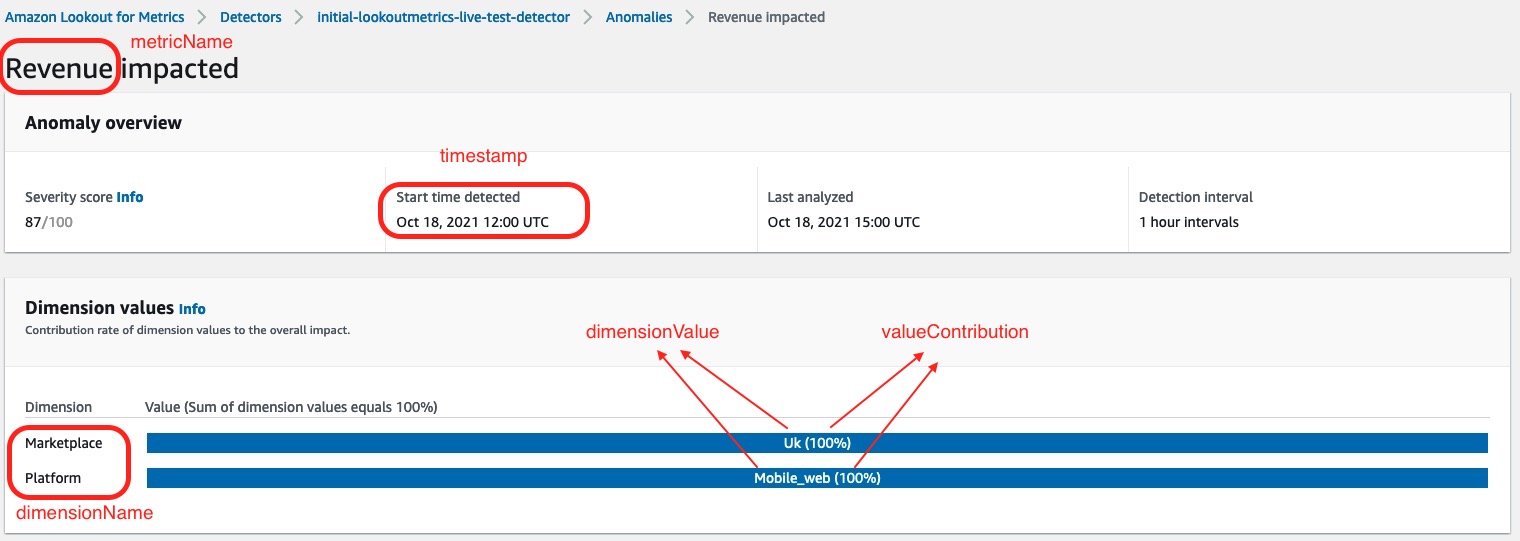
In this post, we use a Lookout for Metrics live detector built following the Getting Started section from the AWS Samples, Amazon Lookout for Metrics GitHub repo. After the detector is active and anomalies are generated from the dataset, we connect Lookout for Metrics to Amazon QuickSight. We create two datasets: one by joining the dimensions table with the anomaly table, and another by joining the anomaly table with the live data. We can then add these two datasets to a QuickSight analysis, where we can add charts in a single dashboard.

We can provide two types of data to the Lookout for Metrics detector: continuous and historical. The AWS Samples GitHub repo offers both, though we focus on the continuous live data. The detector monitors this live data to identify anomalies and writes the anomalies to Amazon Simple Storage Service (Amazon S3) as they’re generated. At the end of a specified interval, the detector analyzes the data. Over time, the detector learns to more accurately identify anomalies based on patterns it finds.

Lookout for Metrics uses machine learning (ML) to automatically detect and diagnose anomalies in business and operational data, such as a sudden dip in sales revenue or customer acquisition rates. The service is now generally available as of March 25, 2021. It automatically inspects and prepares data from a variety of sources to detect anomalies with greater speed and accuracy than traditional methods used for anomaly detection. You can also provide feedback on detected anomalies to tune the results and improve accuracy over time. Lookout for Metrics makes it easy to diagnose detected anomalies by grouping together anomalies related to the same event and sending an alert that includes a summary of the potential root cause. It also ranks anomalies in order of severity so you can prioritize your attention to what matters the most to your business.

QuickSight is a fully-managed, cloud-native business intelligence (BI) service that makes it easy to connect to your data to create and publish interactive dashboards. Additionally, you can use Amazon QuickSight to get instant answers through natural language queries.

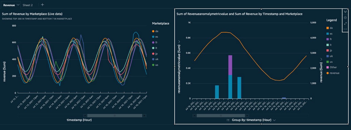
You can access serverless, highly scalable QuickSight dashboards from any device, and seamlessly embed them into your applications, portals, and websites. The following screenshot is an example of what you can achieve by the end of this post.

Overview of solution

The solution is a combination of AWS services, primarily Lookout for Metrics, QuickSight, AWS Lambda, Amazon Athena, AWS Glue, and Amazon S3.

The following diagram illustrates the solution architecture. Lookout for Metrics detects and sends the anomalies to Lambda via an alert. The Lambda function generates the anomaly results as CSV files and saves them in Amazon S3. An AWS Glue crawler analyzes the metadata, and creates tables in Athena. QuickSight uses Athena to query the Amazon S3 data, allowing dashboards to be built to visualize both the anomaly results and the live data.

This solution expands on the resources created in the Getting Started section of the GitHub repo. For each step, we include options to create the resources either using the AWS Management Console or launching the provided AWS CloudFormation stack. If you have a customized Lookout for Metrics detector, you can use it and adapt it the following notebook to achieve the same results.

The implementation steps are as follows:

1. Create the Amazon SageMaker notebook instance (ALFMTestNotebook) and notebooks using the stack provided in the Initial Setup section from the GitHub repo.
2. Open the notebook instance on the SageMaker console and navigate to the amazon-lookout-for-metrics-samples/getting_started folder.
3. Create the S3 bucket and complete the data preparation using the first notebook (1.PrereqSetupData.ipynb). Open the notebook with the conda_python3 kernel, if prompted.

We skip the second notebook because it’s focused on backtesting data.

4. If you’re walking through the example using the console, create the Lookout for Metrics live detector and its alert using the third notebook (3.GettingStartedWithLiveData.ipynb).

If you’re using the provided CloudFormation stacks, the third notebook isn’t required. The detector and its alert are created as part of the stack.

5. After you create the Lookout for Metrics live detector, you need to activate it from the console.

This can take up to 2 hours to initialize the model and detect anomalies.

6. Deploy a Lambda function, using Python with a Pandas library layer, and create an alert attached to the live detector to launch it.
7. Use the combination of Athena and AWS Glue to discover and prepare the data for QuickSight.
8. Create the QuickSight data source and datasets.
9. Finally, create a QuickSight analysis for visualization, using the datasets.

The CloudFormation scripts are typically run as a set of nested stacks in a production environment. They’re provided individually in this post to facilitate a step-by-step walkthrough.

Prerequisites

To go through this walkthrough, you need an AWS account where the solution will be deployed. Make sure that all the resources you deploy are in the same Region. You need a running Lookout for Metrics detector built from notebooks 1 and 3 from the GitHub repo. If you don’t have a running Lookout for Metrics detector, you have two options:

• Run notebooks 1 and 3, and continue from the step 1 of this post (creating the Lambda function and alert)
• Run notebook 1 and then use the CloudFormation template to generate the Lookout for Metrics detector

Create the live detector using AWS CloudFormation

The L4MLiveDetector.yaml CloudFormation script creates the Lookout for Metrics anomaly detector with its source pointing to the live data in the specified S3 bucket. To create the detector, complete the following steps:

1. Launch the stack from the following link:

2. On the Create stack page, choose Next.
3. On the Specify stack details page, provide the following information:
   1. A stack name. For example, L4MLiveDetector.
   2. The S3 bucket, <Account Number>-lookoutmetrics-lab.
   3. The Role ARN, arn:aws:iam::<Account Number>:role/L4MTestRole.
   4. An anomaly detection frequency. Choose PT1H (hourly).
4. Choose Next.
5. On the Configure stack options page, leave everything as is and choose Next.
6. On the Review page, leave everything as is and choose Create stack.

Create the live detector SMS alert using AWS CloudFormation (Optional)

This step is optional. The alert is presented as an example, with no impact on the dataset creation. The L4MLiveDetectorAlert.yaml CloudFormation script creates the Lookout for Metrics anomaly detector alert with an SMS target.

1. Launch the stack from the following link:

2. On the Create stack page, choose Next.
3. On the Specify stack details page, update the SMS phone number and enter a name for the stack (for example, L4MLiveDetectorAlert).
4. Choose Next.
5. On the Configure stack options page, leave everything as is and choose Next.
6. On the Review page, select the acknowledgement check box, leave everything else as is, and choose Create stack.

Resource cleanup

Before proceeding with the next step, stop your SageMaker notebook instance to ensure no unnecessary costs are incurred. It is no longer needed.

Create the Lambda function and alert

In this section, we provide instructions on creating your Lambda function and alert via the console or AWS CloudFormation.

Create the function and alert with the console

You need a Lambda AWS Identity and Access Management (IAM) role following the least privilege best practice to access the bucket where you want the results to be saved.

1. 1. On the Lambda console, create a new function.
   2. Select Author from scratch.
   3. For Function name¸ enter a name.
   4. For Runtime, choose Python 3.8.
   5. For Execution role, select Use an existing role and specify the role you created.
   6. Choose Create function.
2. 
   7. Download the ZIP file containing the necessary code for the Lambda function.
   8. On the Lambda console, open the function.
   9. On the Code tab, choose Upload from, choose .zip file, and upload the file you downloaded.
   10. Choose Save.

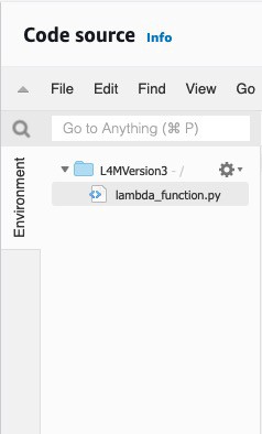
Your file tree should remain the same after uploading the ZIP file.

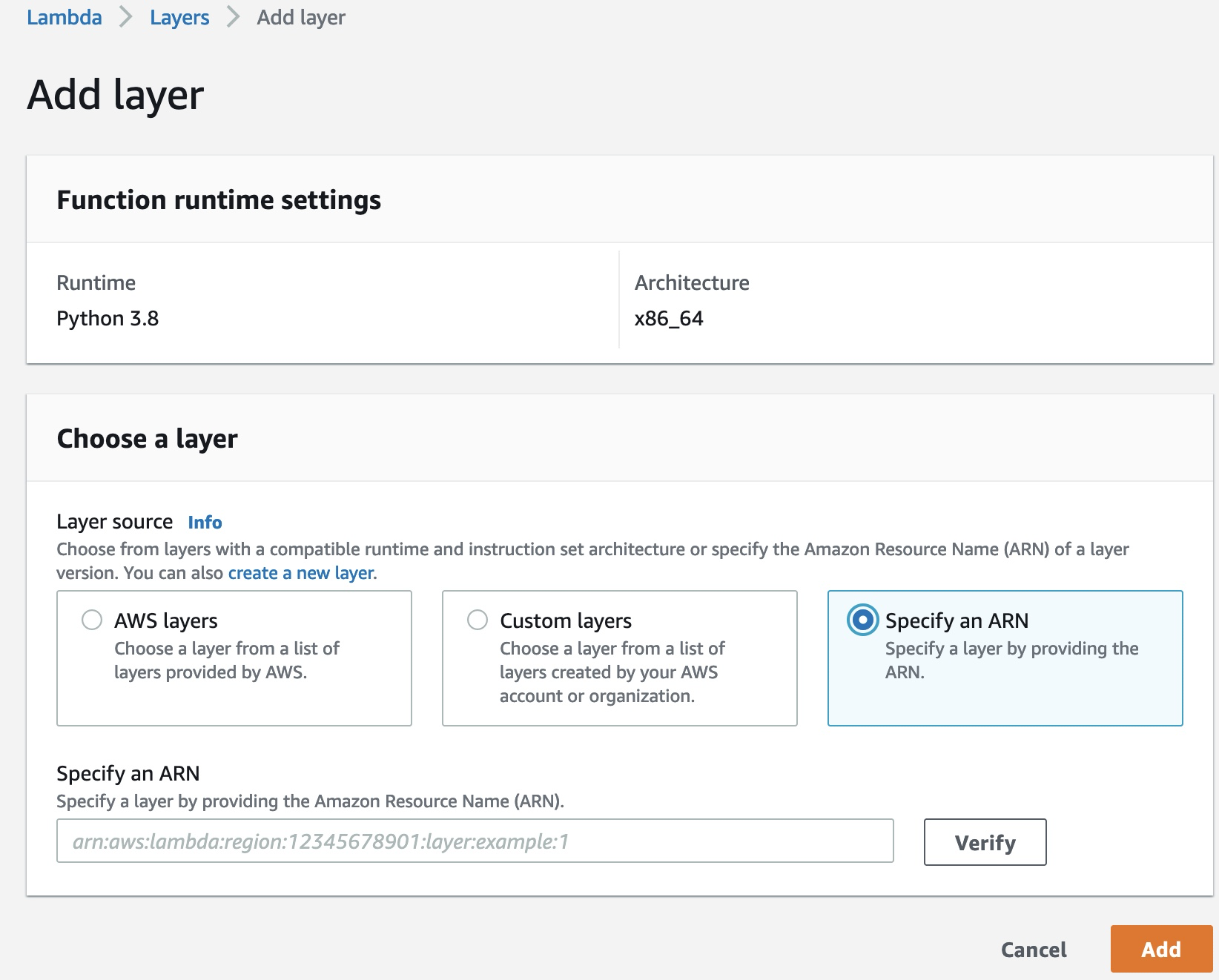
11. In the Layers section, choose Add layer.
12. Select Specify an ARN.
13. In the following GitHub repo, choose the CSV corresponding to the Region you’re working in and copy the ARN from the latest Pandas version.
14. For Specify an ARN, enter the ARN you copied.
15. Choose Add.

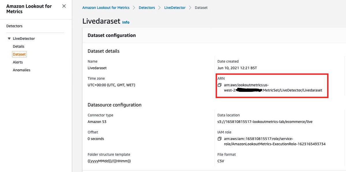
16. To adapt the function to your environment, at the bottom of the code from the lambda_function.py file, make sure to update the bucket name with your bucket where you want to save the anomaly results, and the DataSet_ARN from your anomaly detector.
17. Choose Deploy to make the changes active.

You now need to connect the Lookout for Metrics detector to your function.

18. On the Lookout for Metrics console, navigate to your detector and choose Add alert.
19. Enter the alert name and your preferred severity threshold.
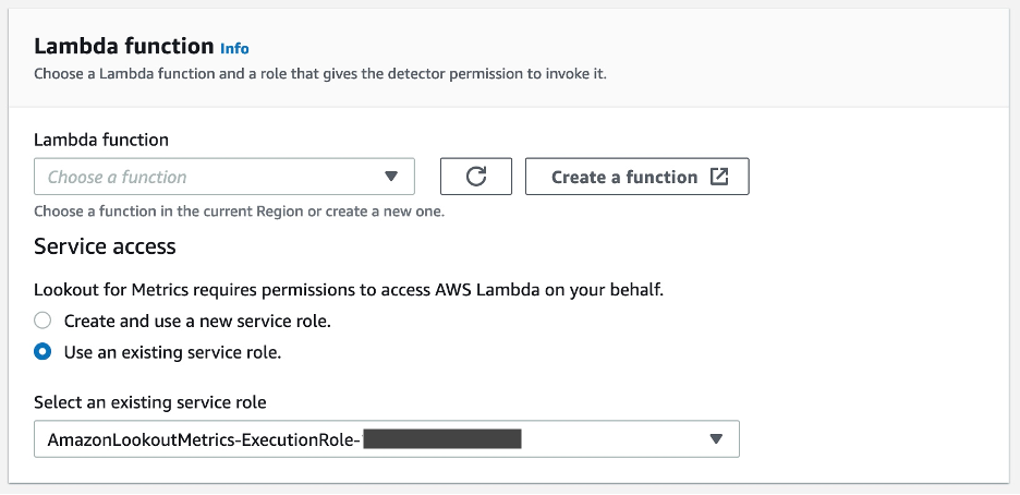
20. From the channel list, choose Lambda.
21. Choose the function you created and make sure you have the right role to trigger it.
22. Choose Add alert.

Now you wait for your alert to trigger. The time varies depending on when the detector finds an anomaly.

When an anomaly is detected, Lookout for Metrics triggers the Lambda function. It receives the necessary information from Lookout for Metrics and checks if there is already a saved CSV file in Amazon S3 at the corresponding timestamp of the anomaly. If there isn’t a file, Lambda generates the file and adds the anomaly data. If the file already exists, Lambda updates the file with the extra data received. The function generates a separated CSV file for each different timestamp.

Create the function and alert using AWS CloudFormation

Similar to the console instructions, you download the ZIP file containing the necessary code for the Lambda function. However, in this case it needs to be uploaded to the S3 bucket in order for the AWS CloudFormation code to load it during function creation.

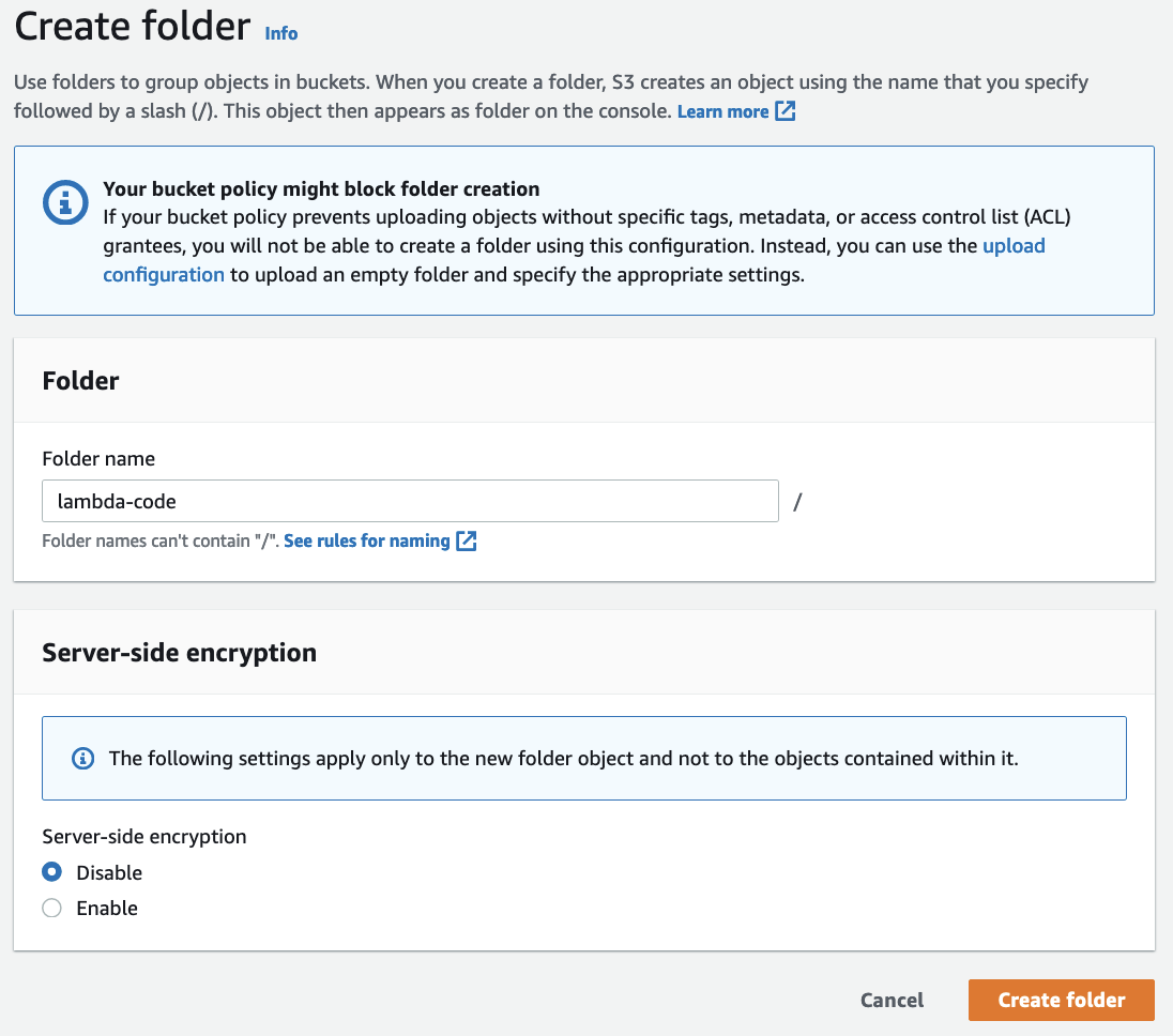
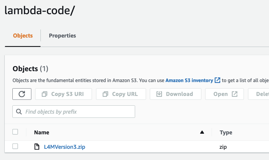
In the S3 bucket specified in the Lookout for Metrics detector creation, create a folder called lambda-code, and upload the ZIP file.

The Lambda function loads this as its code during creation.

The L4MLambdaFunction.yaml CloudFormation script creates the Lambda function and alert resources and uses the function code archive stored in the same S3 bucket.

1. Launch the stack from the following link:

2. On the Create stack page, choose Next.
3. On the Specify stack details page, specify a stack name (for example, L4MLambdaFunction).
4. In the following GitHub repo, open the CSV corresponding to the Region you’re working in and copy the ARN from the latest Pandas version.
5. Enter the ARN as the Pandas Lambda layer ARN parameter.
6. Choose Next.
7. On the Configure stack options page, leave everything as is and choose Next.
8. On the Review page, select the acknowledgement check box, leave everything else as is, and choose Create stack.

Activate the detector

Before proceeding to the next step, you need to activate the detector from the console.

1. On the Lookout for Metrics console, choose Detectors in the navigation pane.
2. Choose your newly created detector.
3. Choose Activate, then choose Activate again to confirm.

Activation initializes the detector; it’s finished when the model has completed its learning cycle. This can take up to 2 hours.

Prepare the data for QuickSight

Before you complete this step, give the detector time to find anomalies. The Lambda function you created saves the anomaly results in the Lookout for Metrics bucket in the anomalyResults directory. We can now process this data to prepare it for QuickSight.

Create the AWS Glue crawler on the console

After some anomaly CSV files have been generated, we use an AWS Glue crawler to generate the metadata tables.

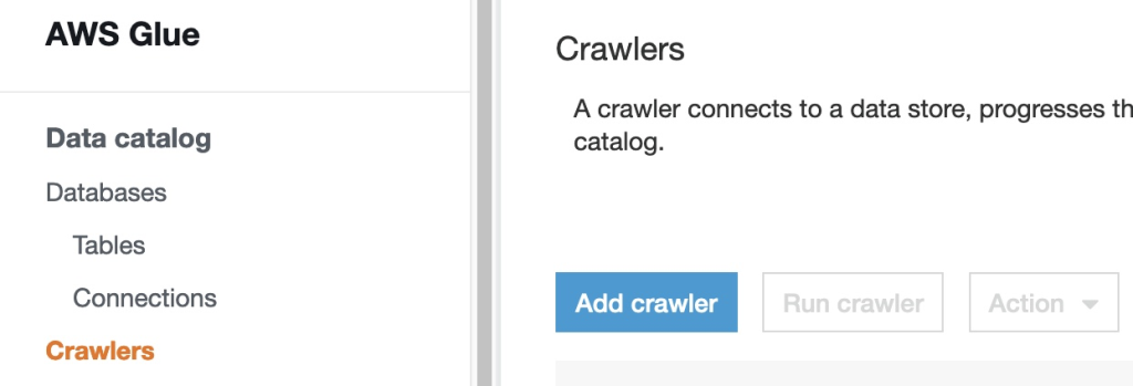
1. On the AWS Glue console, choose Crawlers in the navigation pane.
2. Choose Add crawler.

3. Enter a name for the crawler (for example, L4MCrawler).
4. Choose Next.
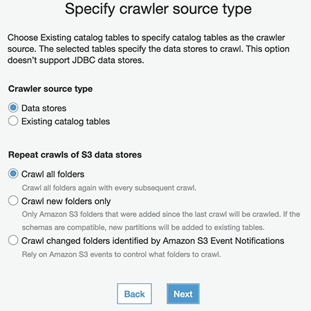
5. For Crawler source type, select Data stores.
6. For Repeat crawls of S3 data stores, select Crawl all folders.
7. Choose Next.

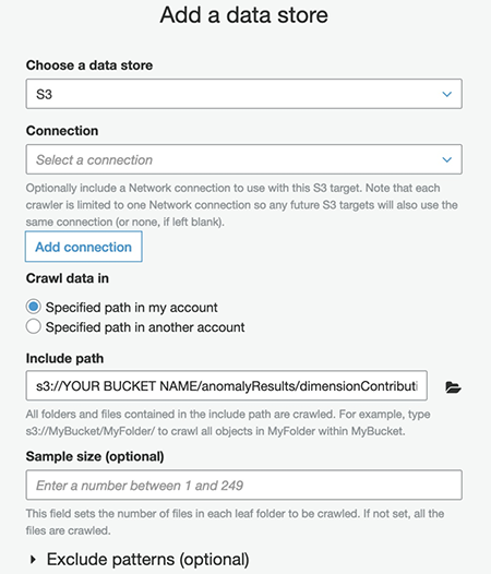
8. On the data store configuration page, for Crawl data in, select Specified path in my account.
9. For Include path, enter the path of your dimensionContributions file (s3://YourBucketName/anomalyResults/dimensionContributions).
10. Choose Next.
11. Choose Yes to add another data store and repeat the instructions for metricValue_AnomalyScore(s3://YourBucketName/anomalyResults/metricValue_AnomalyScore).
12. Repeat the instructions again for the live data to be analyzed by the Lookout for Metrics anomaly detector (this is the S3 dataset location from your Lookout for Metrics detector).

You should now have three data stores for the crawler to process.

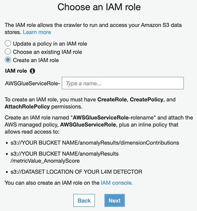
Now you need to select the role to allow the crawler to go through the S3 locations of your data.

13. For this post, select Create an IAM role and enter a name for the role.
14. Choose Next.

15. For Frequency, leave as Run on demand and choose Next.
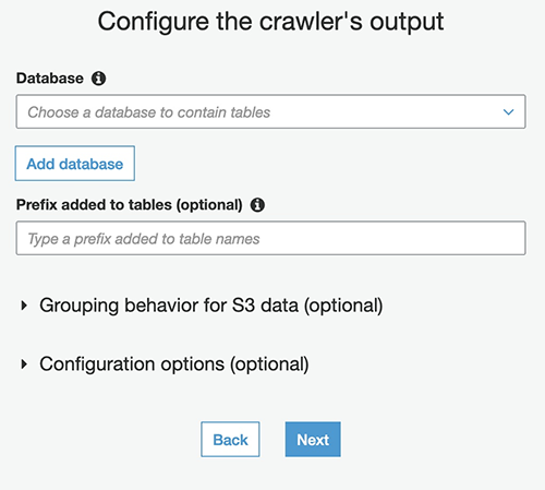
16. In the Configure the crawler’s output section, choose Add database.

This creates the Athena database where your metadata tables are located after the crawler is complete.

17. Enter a name for your database and choose Create.
18. Choose Next, then choose Finish.

19. On the Crawlers page of the AWS Glue console, select the crawler you created and choose Run crawler.

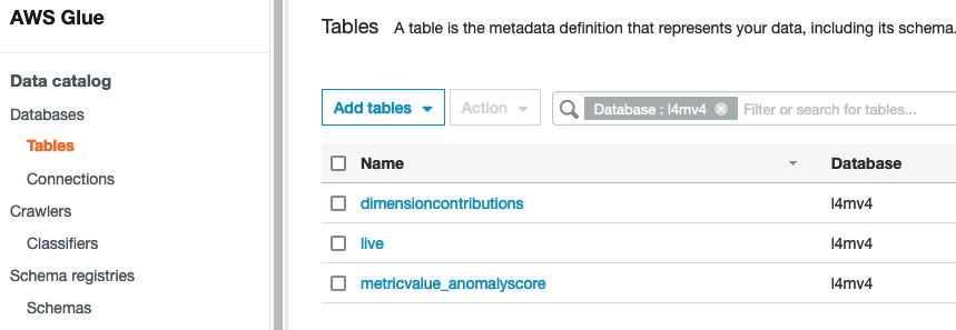
You may need to wait a few minutes, depending on the size of the data. When it’s complete, the crawler’s status shows as Ready. To see the metadata tables, navigate to your database on the Databases page and choose Tables in the navigation pane.

In this example, the metadata table called live represents the S3 dataset from the Lookout for Metrics live detector. As a best practice, it’s recommended to encrypt your AWS Glue Data Catalog metadata.

Athena automatically recognizes the metadata tables, and QuickSight uses Athena to query the data and visualize the results.

Create the AWS Glue crawler using AWS CloudFormation

The L4MGlueCrawler.yaml CloudFormation script creates the AWS Glue crawler, its associated IAM role, and the output Athena database.

1. Launch the stack from the following link:

2. On the Create stack page, choose Next.
3. On the Specify stack details page, enter a name for your stack (for example, L4MGlueCrawler), and choose Next.
4. On the Configure stack options page, leave everything as is and choose Next.
5. On the Review page, select the acknowledgement check box, leave everything else as is, and choose Create stack.

Run the AWS Glue crawler

After you create the crawler, you need to run it before moving to the next step. You can run it from the console or the AWS Command Line Interface (AWS CLI). To use the console, complete the following steps:

1. On the AWS Glue console, choose Crawlers in the navigation pane.
2. Select your crawler (L4MCrawler).
3. Choose Run crawler.

When the crawler is complete, it shows the status Ready.

Create a QuickSight account

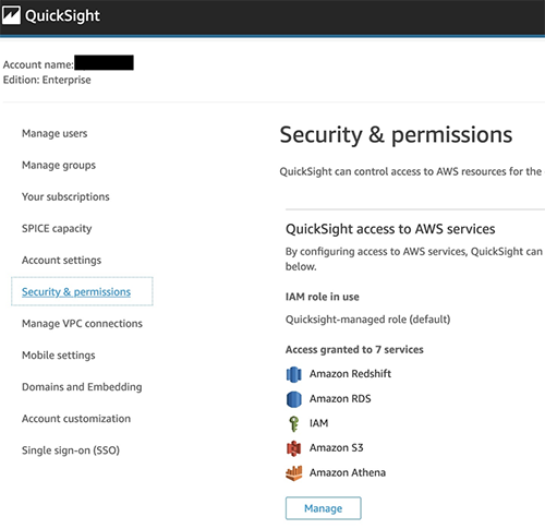
Before starting this next step, navigate to the QuickSight console and create an account if you don’t already have one. To make sure you have access to the corresponding services (Athena and S3 bucket), choose your account name on the top right, choose Manage QuickSight, and choose Security and Permissions, where you can add the necessary services. When setting up your Amazon S3 access, make sure to select Write permission for Athena Workgroup.

Now you’re ready to visualize your data in QuickSight.

Create the QuickSight datasets on the console

If this is your first time using Athena, you have to configure the output location of the queries. For instructions, refer to Steps 1–6 in Create a database. Then complete the following steps:

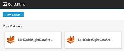
1. On the QuickSight console, choose Datasets.
2. Choose New dataset.
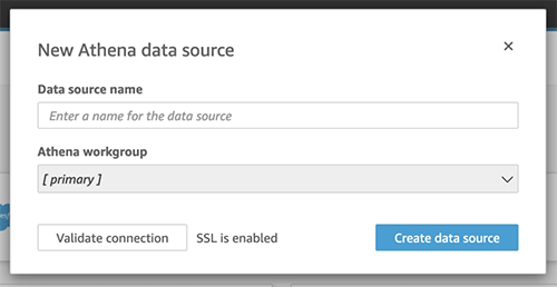
3. Choose Athena as your source.
4. Enter a name for your data source.
5. Choose Create data source.

6. For your database, specify the one you created earlier with the AWS Glue crawler.
7. Specify the table that contains your live data (not the anomalies).
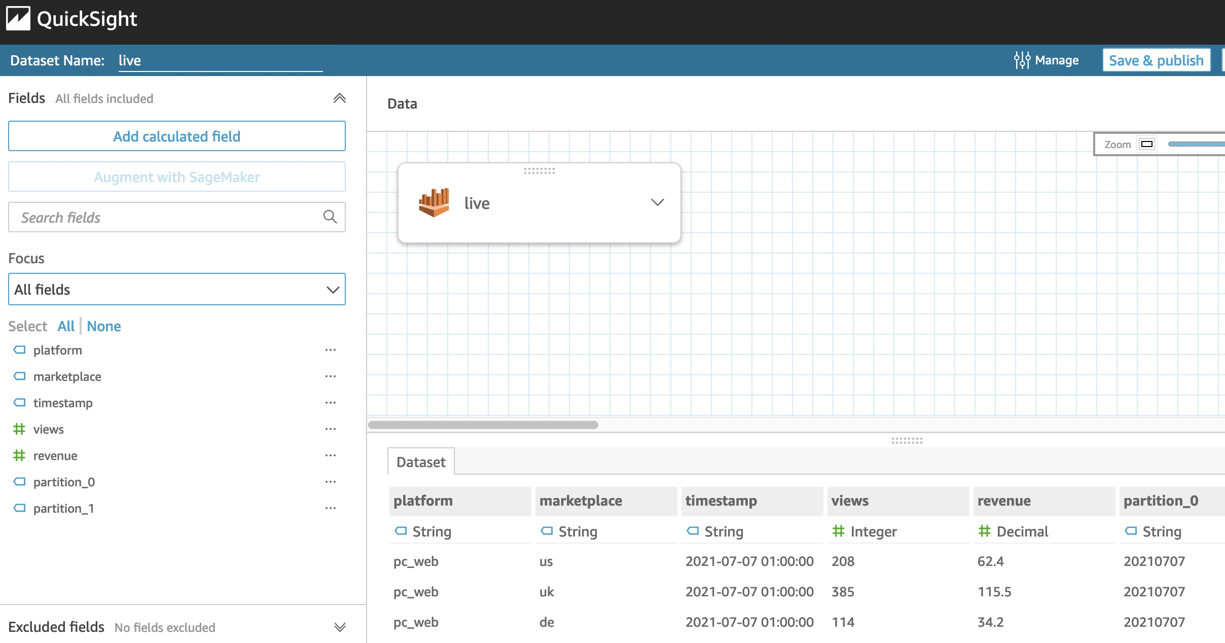
8. Choose Edit/preview data.

You’re redirected to an interface similar to the following screenshot.

The next step is to add and combine the metricValue_AnomalyScore data with the live data.

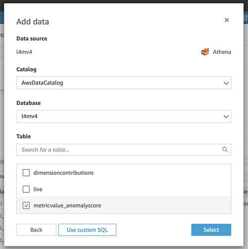
9. Choose Add data.
10. Choose Add data source.
11. Specify the database you created and the metricValue_AnomalyScore table.
12. Choose Select.

You need now to configure the join of the two tables.

13. Choose the link between the two tables.
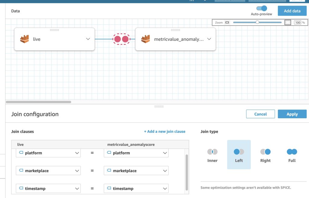
14. Leave the join type as Left, add the timestamp and each dimension you have as a join clause, and choose Apply.

In the following example, we use timestamp, platform, and marketplace as join clauses.

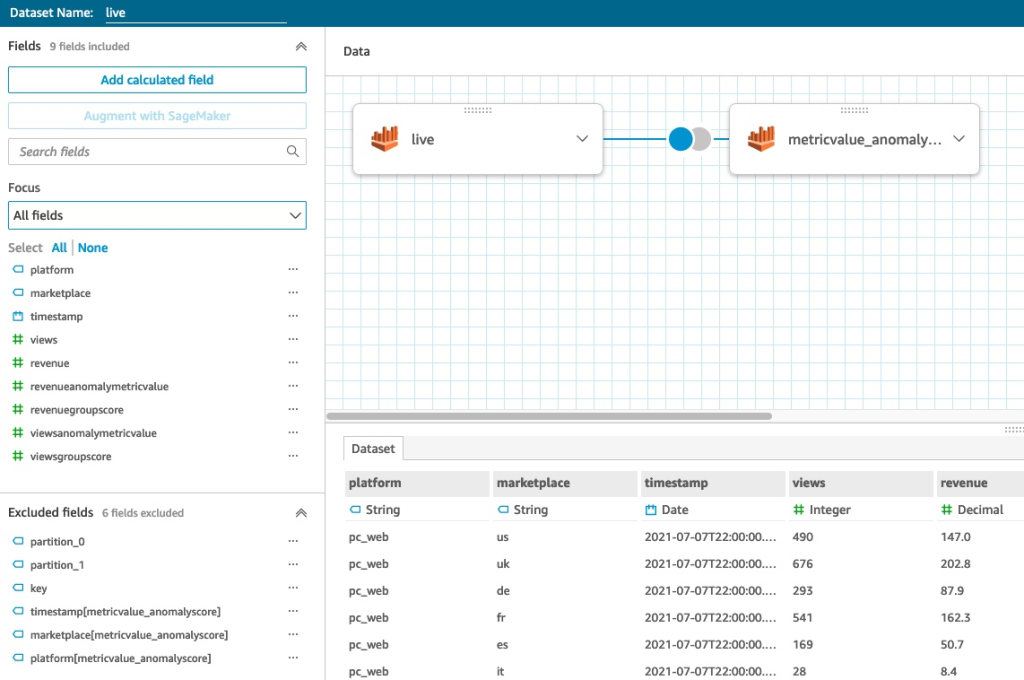
On the right pane, you can remove the fields you’re not interested in keeping.

15. Remove the timestamp from the metricValue_AnomalyScore table to not have a duplicated column.
16. Change the timestamp data type (of the live data table) from string to date, and specify the correct format. In our case, it should be yyyy-MM-dd HH:mm:ss.

The following screenshot shows your view after you remove some fields and adjust the data type.

17. Choose Save and visualize.
18. Choose the pencil icon next to the dataset.
19. Choose Add dataset and choose dimensioncontributions.

Create the QuickSight datasets using AWS CloudFormation

This step contains three CloudFormation stacks.

The first CloudFormation script, L4MQuickSightDataSource.yaml, creates the QuickSight Athena data source.

1. Launch the stack from the following link:

2. On the Create stack page, choose Next.
3. On the Specify stack details page, enter your QuickSight user name, the QuickSight account Region (specified when creating the QuickSight account), and a stack name (for example, L4MQuickSightDataSource).
4. Choose Next.
5. On the Configure stack options page, leave everything as is and choose Next.
6. On the Review page, leave everything as is and choose Create stack.

The second CloudFormation script, L4MQuickSightDataSet1.yaml, creates a QuickSight dataset that joins the dimensions table with the anomaly table.

1. Launch the stack from the following link:

2. On the Create stack page, choose Next.
3. On the Specify stack details, enter a stack name (for example, L4MQuickSightDataSet1).
4. Choose Next.
5. On the Configure stack options page, leave everything as is and choose Next.
6. On the Review page, leave everything as is and choose Create stack.

The third CloudFormation script, L4MQuickSightDataSet2.yaml, creates the QuickSight dataset that joins the anomaly table with the live data table.

1. Launch the stack from the following link:

2. On the Create stack page¸ choose Next.
3. On the Specify stack details page, enter a stack name (for example, L4MQuickSightDataSet2).
4. Choose Next.
5. On the Configure stack options page, leave everything as is and choose Next.
6. On the Review page, leave everything as is and choose Create stack.

Create the QuickSight analysis for dashboard creation

This step can only be completed on the console. After you’ve created your QuickSight datasets, complete the following steps:

1. On the QuickSight console, choose Analysis in the navigation pane.
2. Choose New analysis.
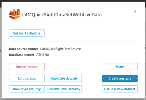
3. Choose the first dataset, L4MQuickSightDataSetWithLiveData.

4. Choose Create analysis.

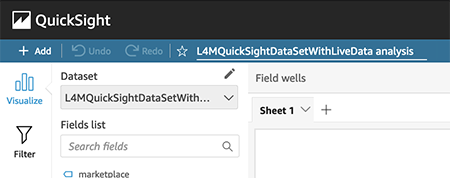
The QuickSight analysis is initially created with only the first dataset.

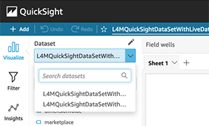
5. To add the second dataset, choose the pencil icon next to Dataset and choose Add dataset.
6. Choose the second dataset and choose Select.

You can then use either dataset for creating charts by choosing it on the Dataset drop-down menu.

Dataset metrics

You have successfully created a QuickSight analysis from Lookout for Metrics inference results and the live data. Two datasets are in QuickSight for you to use: L4M_Visualization_dataset_with_liveData and L4M_Visualization_dataset_with_dimensionContribution.

The L4M_Visualization_dataset_with_liveData dataset includes the following metrics:

• timestamp – The date and time of the live data passed to Lookout for Metrics
• views – The value of the views metric
• revenue – The value of the revenue metric
• platform, marketplace, revenueAnomalyMetricValue, viewsAnomalyMetricValue, revenueGroupScore and viewsGroupScore – These metrics are part of both datasets

The L4M_Visualization_dataset_with_dimensionContribution dataset includes the following metrics:

• timestamp – The date and time of when the anomaly was detected
• metricName – The metrics you’re monitoring
• dimensionName – The dimension within the metric
• dimensionValue – The value of the dimension
• valueContribution – The percentage on how much dimensionValue is affecting the anomaly when detected

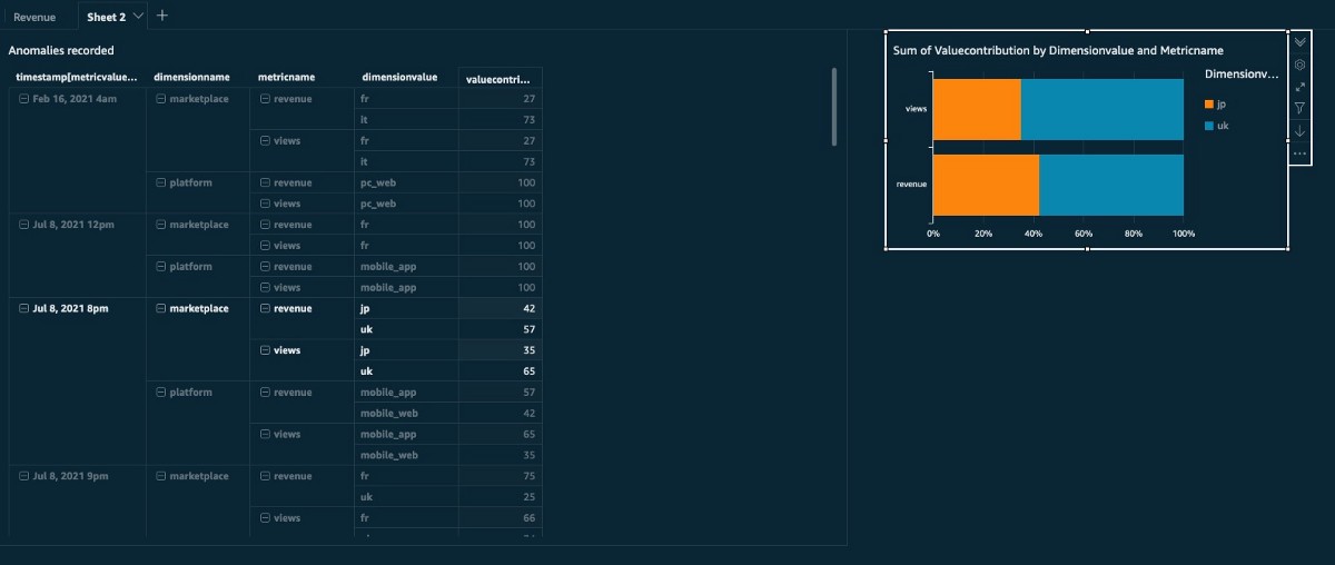
The following screenshot shows these five metrics on the anomaly dashboard of the Lookout for Metrics detector.

The following metrics are part of both datasets:

• platform – The platform where the anomaly happened
• marketplace – The marketplace where the anomaly happened
• revenueAnomalyMetricValue and viewsAnomalyMetricValue – The corresponding values of the metric when the anomaly was detected (in this situation, the metrics are revenue or views)
• revenueGroupScore and viewsGroupScore – The severity scores for each metric for the detected anomaly

To better understand these last metrics, you can review the CSV files created by the Lambda function in your S3 bucket where you saved anomalyResults/metricValue_AnomalyScore.

Next steps

The next step is to build the dashboards for the data you want to see. This post doesn’t include an explanation on creating QuickSight charts. If you’re new to QuickSight, refer to Getting started with data analysis in Amazon QuickSight for an introduction. The following screenshots show examples of basic dashboards. For more information, check out the QuickSight workshops.

Conclusion

The anomalies are presented individually on the Lookout for Metrics console, each with their own graph, making it difficult to view the set as a whole. An automated, integrated solution is needed for deeper analysis. In this post, we used a Lookout for Metrics detector to generate anomalies, and connected the data to QuickSight to create visualizations. This solution enables us to conduct deeper analysis into anomalies and have them all in one single place/dashboard.

As a next step, this solution could as well be expanded by adding an extra dataset and combine anomalies from multiple detectors. You could also adapt the Lambda function. The Lambda function contains the code that generates the data sets and variable names that we use for the QuickSight dashboards. You can adapt this code to your particular use case by changing the data sets itself or the variable names that make more sense to you.

If you have any feedback or questions, please leave them in the comments.

About the Authors

Benoît de Patoul is an AI/ML Specialist Solutions Architect at AWS. He helps customers by providing guidance and technical assistance to build solutions related to AI/ML when using AWS.

Paul Troiano is a Senior Solutions Architect at AWS, based in Atlanta, GA. He helps customers by providing guidance on technology strategies and solutions on AWS. He is passionate about all things AI/ML and solution automation.

Read More

The AWS website is currently available in 16 languages (12 for the AWS Management Console and for technical documentation): Arabic, Chinese Simplified, Chinese Traditional, English, French, German, Indonesian, Italian, Japanese, Korean, Portuguese, Russian, Spanish, Thai, Turkish, and Vietnamese. Customers all over the world gain hands-on experience with the AWS platform, products, and services in their native language. This is made possible thanks to the AWS Localization team (AWSLOC).

AWSLOC manages the end-to-end localization process of digital content at AWS (webpages, consoles, technical documentation, e-books, banners, videos, and more). On average, the team manages 48,000 projects across all digital assets yearly, which amounts to over 3 billion translated words. Given the growing demand of global customers and new local cloud adoption journeys, AWS Localization needs to support content localization at scale, with the aim to make more content available and cater to new markets. To do so, AWSLOC uses a network of over 2,800 linguists globally and supports hundreds of content creators across AWS to scale localization. The team strives to continuously improve the language experience for customers by investing heavily in automation and building automated pipelines for all content types.

AWSLOC aspires to build a future where you can interact with AWS in your preferred language. To achieve this vision, they’re using AWS machine translation and Amazon Translate. The goal is to remove language barriers and make AWS content more accessible through consistent locale-specific experiences to help every AWS creator deliver what matters most to global audiences.

This post describes how AWSLOC uses Amazon Translate to scale localization and offer their services to new locales. Amazon Translate is a neural machine translation service that delivers fast, high-quality, cost-effective, and customizable language translation. Neural machine translation is a form of language translation that uses deep learning models to deliver accurate and natural sounding translation. For more information about the languages Amazon Translate supports, see Supported languages and language codes.

How AWSLOC uses Amazon Translate

The implementation of machine translation allows AWSLOC to speed up the localization process for all types of content. AWSLOC chose AWS technical documentation to jumpstart their machine translation journey with Amazon Translate because it’s one of the pillars of AWS. Around 18% of all customers chose to view technical documentation in their local language in 2021, which is a 27% increase since 2020. In 2020 alone, over 1,435 features and 31 new services were added in technical documentation, which generated an increase of translation volume of 353% in 2021.

To cater to this demand for translated documentation, AWSLOC partnered with Amazon Translate to optimize the localization processes.

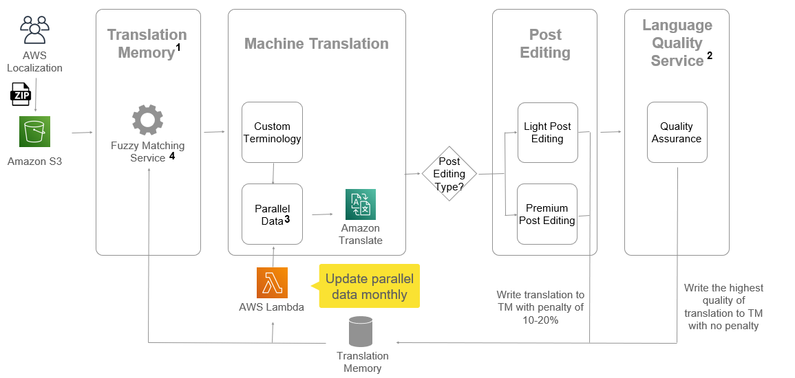
Amazon Translate is used to pre-translate the strings that fall below a fuzzy matching threshold (against the translation memory) across 10 supported languages. A dedicated Amazon Translate instance was configured with Active Custom Translation (ACT) and the corresponding parallel data was updated on a monthly basis. In most of the language pairs, the Amazon Translate plus ACT output has shown a positive trend in quality improvement across the board. Furthermore, to raise the bar on quality, a human post-editing process is then performed on assets that have a higher customer visibility. AWSLOC established a governance process to monitor migration of content across machine translation and machine translation post-editing (MTPE), including MTPE-Light and MTPE-Premium. Human editors review MT outputs to correct translation errors, which are incorporated back into the tool via the ACT process. There is a regular engine refresh (once every 40 days on average), the contributions being mostly bug submissions.

AWSLOC follows best practices to maintain the ACT table, which includes marking some terms with the do not translate feature provided by Amazon Translate.

The following diagram illustrates the detailed workflow.

The main components in the process are as follows:

1. Translation memory – The database that stores sentences, paragraphs, or bullet points that have been previously translated, in order to help human translators. This database stores the source text and its corresponding translation in language pairs, called translation units.
2. Language quality service (LQS) – The accuracy check that an asset goes through after the Language Service Provider (LSP) completes their pass. 20% of the asset is spot-checked unless otherwise specified.
3. Parallel data – The method for analyzing data using parallel processes that run simultaneously on multiple containers.
4. Fuzzy matching – This technique is used in computer-assisted translation as a special case of record linkage. It works with matches that may be less than 100% perfect when finding correspondences between segments of a text and entries in a database of previous translations.
5. Do-not-translate terms – A list of phrases and words that don’t require translation, such as brand names and trademarks.
6. Pre-translation – The initial application of do-not-translate terms, translation memory, and machine translation or human translation engines against a source text before it’s presented to linguists.

MTPE-Light produces understandable but not stylistically perfect text. The following table summarizes the differences between MTPE-Light and MTPE-Premium.

Multi-faceted impacts

Amazon Translate is a solution for localization projects at scale. With Amazon Translate, the project turnaround time isn’t tethered to translation volume. Amazon Translate can deliver more than 50,000 words within 1 hour compared to traditional localization cycles, which can complete 10,000-word projects in 7–8 days and 50,000-word projects in 30–35 days. Amazon Translate is also 10 times cheaper than standard translation, and it makes it easier to track and manage the localization budget. Compared to human translation projects that use MTPE-Premium, AWSLOC observed a savings of up to 40%, and a savings of up to 60% for MTPE-Light. Additionally, projects with machine translation exclusively only incur a monthly flat fee—the technology costs for the translation management system AWSLOC uses to process machine translation.

Lastly, thanks to Amazon Translate, AWSLOC is now able to go from monthly to weekly refresh cycles for technical documentation.

All in all, machine translation is the most cost-effective and time-saving option for any global localization team if they want to cater to an increasing amount of content localization in the long term.

Conclusion

The benefits of Amazon Translate are great to Amazon and to our customers, both in exercising savings and delivering localized content faster and in multiple languages. For more information about the capabilities of Amazon Translate, see the Amazon Translate Developer Guide. If you have any questions or feedback, feel free to contact us or leave a comment.

About the authors

Marie-Alice Daniel is a Language Quality Manager at AWS, based in Luxembourg. She leads a variety of efforts to monitor and improve the quality of localized AWS content, especially Marketing content, with a focus on customer social outreach. She also supports stakeholders to address quality concerns and to ensure localized content consistently meets the quality bar.

Ajit Manuel is a Senior Product Manager (Tech) at AWS, based in Seattle. Ajit leads the localization product management team that builds solutions centered around language analytics services, translation automation and language research and design. The solutions that Ajit’s team builds help AWS scale its global footprint while staying locally relevant. Ajit is passionate about building innovative products especially in niche markets and has pioneered solutions that augmented digital transformation within the insurance-tech and media-analytics space.

Read More

We are excited to announce that Amazon Personalize now supports incremental bulk dataset imports; a new option for updating your data and improving the quality of your recommendations. Keeping your datasets current is an important part of maintaining the relevance of your recommendations. Prior to this new feature launch, Amazon Personalize offered two mechanisms for ingesting data:

• DatasetImportJob – DatasetImportJob is a bulk data ingestion mechanism designed to import large datasets into Amazon Personalize. A typical journey starts with importing your historical interactions dataset in addition to your item catalog and user dataset. DatasetImportJob can then be used to keep your datasets current by sending updated records in bulk. Prior to this launch, data ingested via previous import jobs was overwritten by any subsequent DatasetImportJob.
• Streaming APIs: The streaming APIs (PutEvents, PutUsers, and PutItems) are designed to incrementally update each respective dataset in real-time. For example, after you have trained your model and launched your campaign, your users continue to generate interactions data. This data is then ingested via the PutEvents API, which incrementally updates your interactions dataset. Using the streaming APIs allows you to ingest data as you get it rather than accumulating the data and scheduling ingestion.

With incremental bulk imports, Amazon Personalize simplifies the data ingestion of historical records by enabling you to import incremental changes to your datasets with a DatasetImportJob. You can import 100 GB of data per FULL DatasetImportJob or 1 GB of data per INCREMENTAL DatasetImportJob. Data added to the datasets using INCREMENTAL imports are appended to your existing datasets. Personalize will update records with the current version if your incremental import duplicates any records found in your existing dataset, further simplifying the data ingestion process. In the following sections, we describe the changes to the existing API to support incremental dataset imports.

CreateDatasetImportJob

A new parameter called importMode has been added to the CreateDatasetImportJob API. This parameter is an enum type with two values: FULL and INCREMENTAL. The parameter is optional and is FULL by default to preserve backward compatibility. The CreateDatasetImportJob request is as follows:

{
   "datasetArn": "string",
   "dataSource": { 
      "dataLocation": "string"
   },
   "jobName": "string",
   "roleArn": "string",
   "importMode": {INCREMENTAL, FULL}
}

The Boto3 API is create_dataset_import_job, and the AWS Command Line Interface (AWS CLI) command is create-dataset-import-job.

DescribeDatasetImportJob

The response to DescribeDatasetImportJob has been extended to include whether the import was a full or incremental import. The type of import is indicated in a new importMode field, which is an enum type with two values: FULL and INCREMENTAL. The DescribeDatasetImportJob response is as follows:

{ 
    "datasetImportJob": {
        "creationDateTime": number,
        "datasetArn": "string",
        "datasetImportJobArn": "string",
        "dataSource": {
            "dataLocation": "string"
        },
        "failureReason": "string",
        "jobName": "string",
        "lastUpdatedDateTime": number,
        "roleArn": "string",
        "status": "string",
        "importMode": {INCREMENTAL, FULL}
    }
}

The Boto3 API is describe_dataset_import_job, and the AWS CLI command is describe-dataset-import-job.

ListDatasetImportJob

The response to ListDatasetImportJob has been extended to include whether the import was a full or incremental import. The type of import is indicated in a new importMode field, which is an enum type with two values: FULL and INCREMENTAL. The ListDatasetImportJob response is as follows:

{ 
    "datasetImportJobs": [ { 
        "creationDateTime": number,
        "datasetImportJobArn": "string",
        "failureReason": "string",
        "jobName": "string",
        "lastUpdatedDateTime": number,
        "status": "string",
        "importMode": " {INCREMENTAL, FULL}
    } ],
    "nextToken": "string" 
}

The Boto3 API is list_dataset_import_jobs, and the AWS CLI command is list-dataset-import-jobs.

Code example

The following code shows how to create a dataset import job for incremental bulk import using the SDK for Python (Boto3):

import boto3

personalize = boto3.client('personalize')

response = personalize.create_dataset_import_job(
    jobName = 'YourImportJob',
    datasetArn = 'arn:aws:personalize:us-east 1:111111111111:dataset/AmazonPersonalizeExample/INTERACTIONS',
    dataSource = {'dataLocation':'s3://bucket/file.csv'},
    roleArn = 'role_arn',
    importMode = 'INCREMENTAL'
)

dsij_arn = response['datasetImportJobArn']

print ('Dataset Import Job arn: ' + dsij_arn)

description = personalize.describe_dataset_import_job(
    datasetImportJobArn = dsij_arn)['datasetImportJob']

print('Name: ' + description['jobName'])
print('ARN: ' + description['datasetImportJobArn'])
print('Status: ' + description['status'])

Summary

In this post, we described how you can use this new feature in Amazon Personalize to perform incremental updates to a dataset with bulk import, keeping the data fresh and improving the relevance of Amazon Personalize recommendations. If you have delayed access to your data, incremental bulk import allows you to import your data more easily by appending it to your existing datasets.

Try out this new feature by accessing Amazon Personalize now.

About the authors

Neelam Koshiya is an enterprise solution architect at AWS. Her current focus is to help enterprise customers with their cloud adoption journey for strategic business outcomes. In her spare time, she enjoys reading and being outdoors.

James Jory is a Principal Solutions Architect in Applied AI with AWS. He has a special interest in personalization and recommender systems and a background in ecommerce, marketing technology, and customer data analytics. In his spare time, he enjoys camping and auto racing simulations.

Daniel Foley is a Senior Product Manager for Amazon Personalize. He is focused on building applications that leverage artificial intelligence to solve our customers’ largest challenges. Outside of work, Dan is an avid skier and hiker.

Alex Berlingeri is a Software Development Engineer with Amazon Personalize working on a machine learning powered recommendations service. In his free time he enjoys reading, working out and watching soccer.

Read More

Amazon Rekognition Custom Labels is a fully managed computer vision service that allows developers to build custom models to classify and identify objects in images that are specific and unique to your business. Rekognition Custom Labels doesn’t require you to have any prior computer vision expertise. For example, you can find your logo in social media posts, identify your products on store shelves, classify machine parts in an assembly line, distinguish healthy and infected plants, or detect animated characters in videos.

Developing a custom model to analyze images is a significant undertaking that requires time, expertise, and resources, often taking months to complete. Additionally, it often requires thousands or tens of thousands of hand-labeled images to provide the model with enough data to accurately make decisions. Generating this data can take months to gather and requires large teams of labelers to prepare it for use in machine learning (ML).

Rekognition Custom Labels builds off of the existing capabilities of Amazon Rekognition, which are already trained on tens of millions of images across many categories. Instead of thousands of images, you simply need to upload a small set of training images (typically a few hundred images or less) that are specific to your use case using the Amazon Rekognition console. If the images are already labeled, you can begin training a model in just a few clicks. If not, you can label them directly on the Rekognition Custom Labels console, or use Amazon SageMaker Ground Truth to label them. Rekognition Custom Labels uses transfer learning to automatically inspect the training data, select the right model framework and algorithm, optimize the hyperparameters, and train the model. When you’re satisfied with the model accuracy, you can start hosting the trained model with just one click.

Today we’re happy to announce the launch of the Rekognition Custom Labels model copy feature. This feature allows you to copy your Rekognition Custom Labels models across projects, which can be in the same AWS account or across AWS accounts in the same AWS Region, without retraining the models from scratch. This new capability makes it easier for you to move Rekognition Custom Labels models through various environments such as development, quality assurance, integration, and production without needing to copy the original training and test datasets and retraining the model. You can use the AWS Command Line Interface (AWS CLI) to copy trained models across projects, which can be in the same AWS account or across AWS accounts.

In this post, we show you how to copy models between different AWS accounts in the same AWS Region.

Benefits of the model copy feature

This new feature has the following benefits:

• Multi-account ML-Ops best practices – You can train a model one time and ensure predictable deployment with consistent results across multiple accounts mapped to various environments such as development, quality assurance, integration, and production allowing you to follow ML-Ops best practices within your organization.
• Cost savings and faster deployment – You can quickly copy a trained model between accounts, avoiding the time taken to retrain in every account and saving on the model retraining cost.
• Protect sensitive datasets – You no longer need to share the datasets between different AWS accounts or users. The training data needs to be available only on the AWS account where model training is done. This is very important for certain industries, where data isolation is essential to meet business or regulatory requirements.
• Easy collaboration – Partners or vendors can now easily train Amazon Rekognition Custom Labels model in their own AWS account and share the models with users across AWS accounts.
• Consistent performance – Model performance is now consistent across different AWS accounts. Model training is generally non-deterministic and two models trained with the same dataset does not guarantee the same performance scores and the same predictions. Copying the model helps make sure that the behavior of the copied model is consistent with the source model eliminating the need to re-test the model.

Solution overview

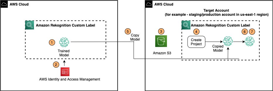
The following diagram illustrates our solution architecture.

This post assumes you have a trained a Rekognition Custom Labels model in your source account. For instructions, refer to Training a custom single class object detection model with Amazon Rekognition Custom Labels. In this post, we used the image classification “Rooms” project from the Rekognition Custom Labels sample projects list and trained a room classification model in the source account to classify images of kitchens, bathrooms, living rooms, and more.

To demonstrate the functionality of the model copy feature, we go through the following steps in the source account:

1. Start the model and run inferences on sample images.
2. Define a resource-based policy to allow cross-account access to copy the Rekognition Custom Labels model.

Then we copy the source model to the target account.

3. Create an Amazon Simple Storage Service (Amazon S3) bucket, which serves as a container for the model evaluation and performance statistics.
4. Create a project.
5. Copy the trained model from the source account to the target account.
6. Start the model and run inference on the sample images.
7. Verify the inference results match the results of the source account model.

Prerequisites

In addition to having a trained model in your source account, make sure you complete the following prerequisite steps:

1. Install the AWS CLI V2.
2. Configure your AWS CLI with the following code and enter your Region:

   aws configure

3. Run the following commands to ensure you have AWS CLI version 2.xx installed on your local host:

   aws --version

4. Update the AWS credentials file under $HOME/.aws/credentials with the following entry:

   [source-account]
   aws_access_key_id = ####
   aws_secret_access_key = #######
   
   [target-account]
   aws_access_key_id = ####
   aws_secret_access_key = #######

5. Get the ProjectArn and ProjectVersionArn for the source AWS account.ProjectArn is the project associated with your source model. ProjectVersionArn is the version of the model you’re interested in copying to the target account.You can find the SourceProjectArn using the following command:

   aws rekognition describe-projects 
   --region us-east-1 
   --profile source-account
   
   {
       "ProjectDescriptions": [{
           "ProjectArn": "arn:aws:rekognition:us-east-1::111111111111:project/rooms_1/1657588855531",
           .
           .
       }]
   }

   If you see multiple lines of output, pick the ProjectArn associated with the model you’re going to copy.

   You can find the SourceProjectVersionArn for the model you trained using the SourceProjectArn (the preceding output). Replace the SourceProjectArn in the following command:

   aws rekognition describe-project-versions 
   --project-arn SourceProjectArn 
   --region us-east-1 
   --profile source-account

   The command returns the SourceProjectVersionArn. If you see multiple lines of output, pick the ProjectVersionArn of interest.

   {
       "ProjectVersionDescriptions": [
           {
               "ProjectVersionArn": "arn:aws:rekognition:us-east-1:111111111111:project/rooms_1/version/rooms_1.2022-07-12T09.39.36/1657643976475",
               .
               .
           }
       ]
   }

You’re now ready to run the steps to implement the solution. Replace the values of SourceProjectArn and SourceProjectVersionArn in the following commands with the values you generated.

1. Start the model and run inference on sample images

In the source account, enter the following code to start the model:

aws rekognition start-project-version 
--project-version-arn SourceProjectVersionArn 
--min-inference-units 1 
--region us-east-1 
--profile source-account
{
    "Status": "STARTING"
}

After the model is hosted and in the running state, you can run inference.

We used the following images (demo1.jpeg and demo2.jpeg) to run inference. These images are located in our local file system in the same directory where the AWS CLI commands are being run from.

The following image is demo1.jpeg, which shows a backyard.

See the following inference code and output:

aws rekognition detect-custom-labels 
--project-version-arn SourceProjectVersionArn   
--image-bytes fileb://demo1.jpeg 
--region us-east-1 
--profile source-account
{
    "Name": "backyard",
    "Confidence": 45.77000045776367
 }

The following image is demo2.jpeg, which shows a bedroom.

See the following inference code and output:

aws rekognition detect-custom-labels 
--project-version-arn SourceProjectVersionArn   
--image-bytes fileb://demo2.jpeg 
--region us-east-1 
--profile source-account
{
    "Name": "bedroom",
    "Confidence": 61.84600067138672
 }

The inference results show the image belongs to the classes backyard and bedroom, with a confidence score of 45.77 and 61.84, respectively.

2. Define the IAM resource policy for the trained model to allow cross-account access

To create your resource-based IAM policy, complete the following steps in the source account:

1. Allow your specific AWS account to access resources using the provided IAM resource policy (for more information, refer to Creating a project policy document. Replace the values for TargetAWSAccountId and SourceProjectVersionArn in the following policy:

   {
       "Version": "2012-10-17",
       "Statement": [
           {
               "Principal": {
                   "AWS": [ "TargetAWSAccountId" ]
               },
               "Action": "Rekognition:CopyProjectVersion",
               "Resource": "SourceProjectVersionArn",
               "Effect": "Allow"
           }
       ]
   }

2. Attach the policy to the project in the source account by calling the following command.

   aws rekognition put-project-policy 
   --project-arn SourceProjectArn 
   --policy-name PolicyName 
   --policy-document '{
       "Version": "2012-10-17",
       "Statement": [
           {
               "Principal": {
                   "AWS": [ "TargetAWSAccountId" ]
               },
               "Action": "Rekognition:CopyProjectVersion",
               "Resource": "SourceProjectVersionArn",
               "Effect": "Allow"
           }
       ]
   }' 
   --region us-east-1 
   --profile source-account

   Replace SourceProjectArn, PolicyName, TargetAWSAccountId, and SourceProjectVersionArn.

   The output shows the policy revision ID created:

   {
       "PolicyRevisionId": "f95907f9c1472c114f61b0e1f31ed131"
   }

Now we’re ready to copy the trained model from the source account to the target account.

3. Create an S3 bucket in the target account

You can use an existing S3 bucket in your account or create a new S3 bucket. For this post, we call this S3 bucket DestinationS3Bucket.

4. Create a new Rekognition Custom Labels project

Create a new project with the following code:

aws rekognition create-project 
--project-name target_rooms_1 
--region us-east-1 
--profile target-account 

This creates a TargetProjectArn in the target account:

{
    "ProjectArn": "arn:aws:rekognition:us-east-1:222222222222:project/target_rooms_1/1657599660206"
}

Note the value of the destination project ProjectArn field. We use this value in the following copy model command.

5. Copy the model from the source account to the target account

Supply the source and target ProjectArn, source ProjectVersionArn, and target S3 bucket and S3 key prefix in the following code:

aws rekognition copy-project-version 
--source-project-arn SourceProjectArn 
--source-project-version-arn SourceProjectVersionArn 
--destination-project-arn TargetProjectArn 
--version-name TargetVersionName 
--output-config '{"S3Bucket":"DestinationS3Bucket", "S3KeyPrefix":"DestinationS3BucketPrefix"}' 
--region us-east-1 
--profile target-account

This creates a copied model TargetProjectVersionArn in the target account. The TargetVersionName in our case has been named copy_rooms_1:

{
    "ProjectVersionArn": "arn:aws:rekognition:us-east-1:222222222222:project/target_rooms_1/version/copy_rooms_1/1657667877079"
}

Check the status of the model copy process:

aws rekognition describe-project-versions 
--project-arn TargetProjectArn 
--version-names TargetVersionName 
--region us-east-1 
--profile target-account

The model copy from the source account to the target account is complete when the Status changes to COPYING_COMPLETED:

 {
    "ProjectVersionDescriptions": [
        {
            "ProjectVersionArn": "arn:aws:rekognition:us-east-1:222222222222:project/target_rooms_1/version/copy_rooms_1/1657667877079",
            "CreationTimestamp": "2022-07-12T16:17:57.079000-07:00",
            "Status": "COPYING_COMPLETED",
            "StatusMessage": "Model copy operation was successful",
            ..........
            ..........
            "EvaluationResult": {
                "F1Score": 0.0,
                "Summary": {

6. Start the model and run inference

Enter the following code to start the model in the target account:

aws rekognition start-project-version 
--project-version-arn TargetProjectArn 
--min-inference-units 1 
--region us-east-1 
--profile target-account
{
    "Status": "STARTING"
}

Check the status of the model:

aws rekognition describe-project-versions 
--project-arn TargetProjectArn 
--version-names copy_rooms_1 
--region us-east-1 
--profile target-account

The model is now hosted and running:

{
    "ProjectVersionDescriptions": [
        {
            "ProjectVersionArn": "arn:aws:rekognition:us-east-1:222222222222:project/target_rooms_1/version/copy_rooms_1/1657667877079",
            "CreationTimestamp": "2022-07-12T16:17:57.079000-07:00",
            "MinInferenceUnits": 1,
            "Status": "RUNNING",
            "StatusMessage": "The model is running.",
            ..........
            ..........
        }
    ]
}

Run inference with the following code:

aws rekognition detect-custom-labels 
 --project-version-arn TargetProjectVersionArn 
 --image-bytes fileb://demo1.jpeg 
 --region us-east-1 
 --profile target-account
{
    "Name": "backyard",
    "Confidence": 45.77000045776367
 }
aws rekognition detect-custom-labels 
 --project-version-arn TargetProjectVersionArn 
 --image-bytes fileb://demo2.jpeg 
 --region us-east-1 
 --profile target-account
{
    "Name": "bedroom",
    "Confidence": 61.84600067138672

7. Verify the inference results match

The classes and the confidence scores for the images demo1.jpg and demo2.jpg in the target account should match the results in the source account.

Conclusion

In this post, we demonstrated the Rekognition Custom Label model copy feature. This feature enables you to train a classification or object detection model in one account and then share the model with another account in the same Region. This simplifies the multi-account strategy where the model can be trained one time and shared between accounts within the same Region without having to retrain or share the training datasets. This allows for a predicable deployment in every account as part of your MLOps workflow. For more information, refer to Copying an Amazon Rekognition Custom Labels model, or try out the walkthrough in this post using a cloud shell with the AWS CLI.

As of this writing, the model copy feature in Amazon Rekognition Custom Labels is available in the following Regions:

• US East (Ohio)
• US East (N. Virginia)
• US West (Oregon)
• Asia Pacific (Mumbai)
• Asia Pacific (Seoul)
• Asia Pacific (Singapore)
• Asia Pacific (Sydney)
• Asia Pacific (Tokyo)
• EU (Frankfurt)
• EU (Ireland)
• EU (London)

Give the feature a try, and please send us feedback either via the AWS forum for Amazon Rekognition or through your AWS support contacts.

About the authors

Amit Gupta is a Senior AI Services Solutions Architect at AWS. He is passionate about enabling customers with well-architected machine learning solutions at scale.

Yogesh Chaturvedi is a Solutions Architect at AWS with a focus in computer vision. He works with customers to address their business challenges using cloud technologies. Outside of work, he enjoys hiking, traveling, and watching sports.

Aakash Deep is a Senior Software Engineer with AWS. He enjoys working on computer vision, AI, and distributed systems. Outside of work, he enjoys hiking and traveling.

Pashmeen Mistry is the Senior Product Manager for Amazon Rekognition Custom Labels. Outside of work, Pashmeen enjoys adventurous hikes, photography, and spending time with his family.

Read More

Medical imaging techniques like computed tomography (CT), magnetic resonance imaging (MRI), medical x-ray imaging, ultrasound imaging, and others are commonly used by doctors for various reasons. Some examples include detecting changes in the appearance of organs, tissues, and vessels, and detecting abnormalities such as tumors and various other type of pathologies.

Before doctors can use the data from those techniques, the data needs to be transformed from its native raw form to a form that can be displayed as an image on a computer screen.

This process is known as image reconstruction, and it plays a crucial role in a medical imaging workflow—it’s the step that creates diagnostic images that can be then reviewed by doctors.

In this post, we discuss a use case of MRI reconstruction, but the architectural concepts can be applied to other types of image reconstruction.

Advances in the field of image reconstruction have led to the successful application of AI-based techniques within magnetic resonance (MR) imaging. These techniques are aimed at increasing the accuracy of the reconstruction and in the case of MR modality, and decreasing the time required for a full scan.

Within MR, applications using AI to work with under-sampled acquisitions have been successfully employed, achieving nearly ten times reduction in scan times.

Waiting times for tests like MRIs and CT scans have increased rapidly in the last couple of years, leading to wait times as long as 3 months. To ensure good patient care, the increasing need for quick availability of reconstructed images along with the need to reduce operational costs has driven the need of a solution capable of scaling according to storage and computational needs.

In addition to computational needs, data growth has seen a steady increase in the last few years. For example, looking at the datasets made available by the Medical Image Computing and Computer-Assisted Intervention (MICCAI), it’s possible to gather that the annual growth is 21% for MRI, 24% for CT, and 31% for functional MRI (fMRI). (For more information, refer to Dataset Growth in Medical Image Analysis Research.)

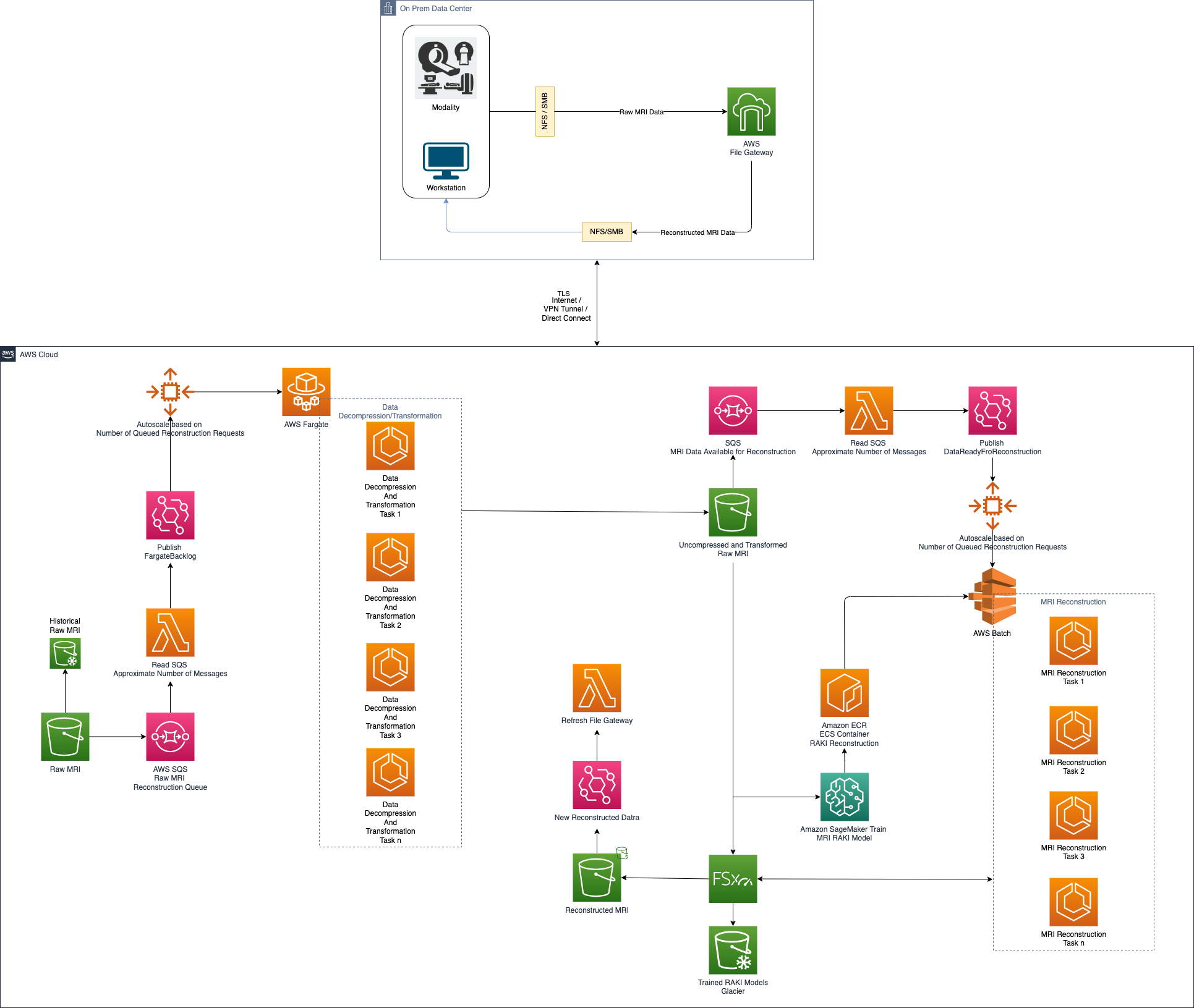
In this post, we show you a solution architecture that addresses these challenges. This solution can enable research centers, medial institutions, and modality vendors to have access to unlimited storage capabilities, scalable GPU power, fast data access for machine learning (ML) training and reconstruction tasks, simple and fast ML development environments, and the ability to have on-premises caching for fast and low-latency image data availability.

Solution overview

This solution uses an MRI reconstruction technique known as Robust Artificial-neural-networks for k-space Interpolation (RAKI). This approach is advantageous because it’s scan-specific and doesn’t require prior data to train the neural network. The drawback to this technique is that it requires a lot of computational power to be effective.

The AWS architecture outlined shows how a cloud-based reconstruction approach can effectively perform computational-heavy tasks like the one required by the RAKI neural network, scaling according to the load and accelerating the reconstruction process. This opens the door to techniques that can’t realistically be implemented on premises.

Data layer

The data layer has been architected around the following principles:

• Seamless integration with modalities that store data generated into an attached storage drive via a network share on a NAS device
• Limitless and secure data storage capabilities to scale to the continuous demand of storage space
• Fast storage availability for ML workloads such as deep neural training and neural image reconstruction
• The ability to archive historic data using a low-cost, scalable approach
• Permit availability to the most frequently accessed reconstructed data while simultaneously keeping less frequently accessed data archived at a lower cost

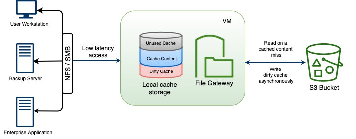
The following diagram illustrates this architecture.

This approach uses the following services:

• AWS Storage Gateway for a seamless integration with the on-premises modality that exchanges information via a file share system. This allows transparent access to the following AWS Cloud storage capabilities while maintaining how the modality exchanges data:
  • Fast cloud upload of the volumes generated by the MR modality.
  • Low-latency access to frequently used reconstructed MR studies via local caching offered by Storage Gateway.
• Amazon SageMaker for unlimited and scalable cloud storage. Amazon S3 also provides low-cost, historical raw MRI data deep archiving with Amazon S3 Glacier, and an intelligent storage tier for the reconstructed MRI with Amazon S3 Intelligent-Tiering.
• Amazon FSx for Lustre for fast and scalable intermediate storage used for ML training and reconstruction tasks.

The following figure shows a concise architecture describing the data exchange between the cloud environments.

Using Storage Gateway with the caching mechanism allows on-premises applications to quickly access data that’s available on the local cache. This occurs while simultaneously giving access to scalable storage space on the cloud.

With this approach, modalities can generate raw data from acquisition jobs, as well as write the raw data into a network share handled from Storage Gateway.

If the modality generates multiple files that belong to the same scan, it’s recommended to create a single archive (.tar for example), and perform a single transfer to the network share to accelerate the data transfer.

Data decompression and transformation layer

The data decompression layer receives the raw data, automatically performs decompression, and applies potential transformations to the raw data before submitting the preprocessed data to the reconstruction layer.

The adopted architecture is outlined in the following figure.

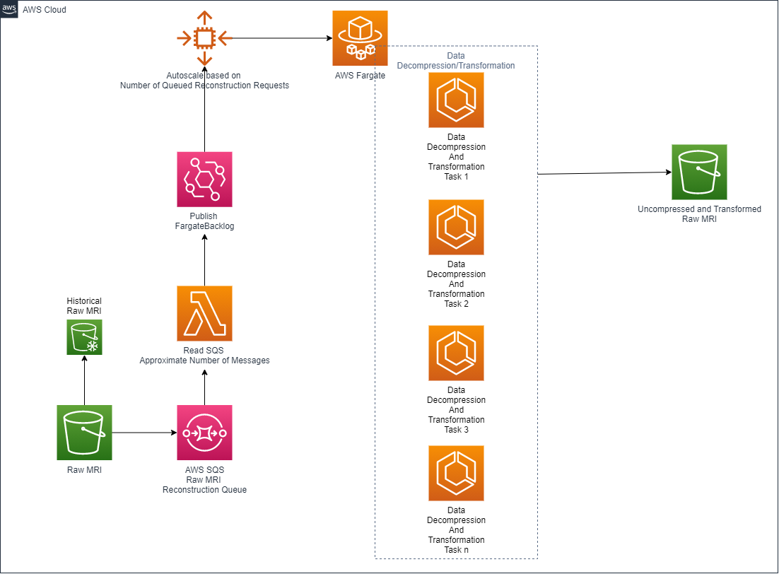
In this architecture, raw MRI data lands in the raw MRI S3 bucket, thereby triggering a new entry in Amazon Simple Queue Service (Amazon SQS).

An AWS Lambda function retrieves the raw MRI Amazon SQS queue depth, which represents the amount of raw MRI acquisitions uploaded to the AWS Cloud. This is used with AWS Fargate to automatically modulate the size of an Amazon Elastic Container Service (Amazon ECS) cluster.

This architecture approach lets it automatically scale up and down accordingly to the number of raw scans landed into the raw input bucket.

After the raw MRI data is decompressed and preprocessed, it’s saved into another S3 bucket so that it can be reconstructed.

Neural model development layer

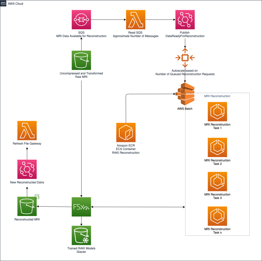
The neural model development layer consists of a RAKI implementation. This creates a neural network model to allow the fast image reconstruction of under-sampled magnetic resonance raw data.

The following figure shows the architecture that realizes the neural model development and container creation.

In this architecture, Amazon SageMaker is used to develop the RAKI neural model, and simultaneously to create the container that is later used to perform the MRI reconstruction.

Then, the created container is included in the fully managed Amazon Elastic Container Registry (Amazon ECR) repository so that it can then spin off reconstruction tasks.

Fast data storage is guaranteed by the adoption of Amazon FSx for Lustre. It provides sub-millisecond latencies, up to hundreds of GBps of throughput, and up to millions of IOPS. This approach gives SageMaker access to a cost-effective, high-performance, and scalable storage solution.

MRI reconstruction layer

The MRI reconstruction based on the RAKI neural network is handled by the architecture shown in the following diagram.

With the same architectural pattern adopted in the decompression and preprocessing layer, the reconstruction layer automatically scales up and down by analyzing the depth of the queue responsible for holding all the reconstruction requests. In this case, to enable GPU support, AWS Batch is used to run the MRI reconstruction jobs.

Amazon FSx for Lustre is used to exchange the large amount of data involved in MRI acquisition. Furthermore, when a reconstruction job is complete and the reconstructed MRI data is stored in the target S3 bucket, the architecture employed automatically requests a refresh of the storage gateway. This makes the reconstructed data available to the on-premises facility.

Overall architecture and results

The overall architecture is shown in the following figure.

We applied the described architecture on MRI reconstruction tasks with datasets approximately 2.4 GB in size.

It took approximately 210 seconds to train 221 datasets, for a total of 514 GB of raw data on a single node equipped with a Nvidia Tesla V100-SXM2-16GB.

The reconstruction, after the RAKI network has been trained, took an average of 40 seconds on a single node equipped with a Nvidia Tesla V100-SXM2-16GB.

The application of the preceding architecture to a reconstruction job can yield the results in the following figure.

The image shows that good results can be obtained via reconstruction techniques such as RAKI. Moreover, adopting cloud technology can make these computation-heavy approaches available without the limitations found in on-premises solutions where storage and computational resources are always limited.

Conclusions

With tools such as Amazon SageMaker, Amazon FSx for Lustre, AWS Batch, Fargate, and Lambda, we can create a managed environment that is scalable, secure, cost-effective, and capable of performing complex tasks such as image reconstruction at scale.

In this post, we explored a possible solution for image reconstruction from raw modality data using a computationally intensive technique known as RAKI: a database free deep learning technique for fast image reconstruction.

To learn more about how AWS is accelerating innovation in healthcare, visit AWS for Health.

References

• Scan-specific Robust Artificial-neural-networks for k-space Interpolation (RAKI): Database free Deep Learning Reconstruction for Fast Imaging
• MRI datasets used in this post

About the author

Benedetto Carollo is the Senior Solution Architect for medical imaging and healthcare at Amazon Web Services in Europe, Middle East, and Africa. His work focuses on helping medical imaging and healthcare customers solve business problems by leveraging technology. Benedetto has over 15 years of experience of technology and medical imaging and has worked for companies like Canon Medical Research and Vital Images. Benedetto received his summa cum laude MSc in Software Engineering from the University of Palermo – Italy.

Read More

Today, we are excited to announce Promotions feature in Amazon Personalize that allows you to explicitly recommend specific items to your users based on rules that align with your business goals. For instance, you can have marketing partnerships that require you to promote certain brands, in-house content, or categories that you want to improve the visibility of. Promotions give you more control over recommended items. You can define business rules to identify promotional items and showcase them across your entire user base, without any extra cost. You also control the percentage of the promoted content in your recommendations. Amazon Personalize automatically finds the relevant items within the set of promotional items that meet your business rule and distributes them within each user’s recommendations.

Amazon Personalize enables you to improve customer engagement by powering personalized product and content recommendations in websites, applications, and targeted marketing campaigns. You can get started without any prior machine learning (ML) experience, using APIs to easily build sophisticated personalization capabilities in a few clicks. All your data is encrypted to be private and secure, and is only used to create recommendations for your users.

In this post, we demonstrate how to customize your recommendations with the new promotions feature for an ecommerce use case.

Solution overview

Different businesses can use promotions based on their individual goals for the type of content they want to increase engagement on. You can use promotions to have a percentage of your recommendations be of a particular type for any application regardless of the domain. For example, in ecommerce applications, you can use this feature to have 20% of recommended items be those marked as on sale, or from a certain brand, or category. For video-on-demand use cases, you can use this feature to fill 40% of a carousel with newly launched shows and movies that you want to highlight, or to promote live content. You can use promotions in domain dataset groups and custom dataset groups (User-Personalization and Similar-Items recipes).

Amazon Personalize makes configuring promotions simple: first, create a filter that selects the items you want promoted. You can use the Amazon Personalize console or API to create a filter with your logic using the Amazon Personalize DSL (domain-specific language). It only takes a few minutes. Then, when requesting recommendations, specify the promotion by specifying the filter, the percentage of the recommendations that should match that filter, and, if required, the dynamic filter parameters. The promoted items are randomly distributed in the recommendations, but any existing recommendations aren’t removed.

The following diagram shows how you can use promotions in recommendations in Amazon Personalize.

You define the items to promote in the catalog system, load them to the Amazon Personalize items dataset, and then get recommendations. Getting recommendations without specifying a promotion returns the most relevant items, and in this example, only one item from the promoted items. There is no guarantee of promoted items being returned. Getting recommendations with 50% promoted items returns half the items belonging to the promoted items.

This post walks you through the process of defining and applying promotions in your recommendations in Amazon Personalize to ensure the results from a campaign or recommender contain specific items that you want users to see. For this example, we create a retail recommender and promote items with CATEGORY_L2 as halloween, which corresponds to Halloween decorations. A code sample for this use case is available on GitHub.

Prerequisites

To use promotions, you first set up some Amazon Personalize resources on the Amazon Personalize console. Create your dataset group, load your data, and train a recommender. For full instructions, see Getting started.

1. Create a dataset group.
2. Create an Interactions dataset using the following schema:

   {
       "type": "record",
       "name": "Interactions",
       "namespace": "com.amazonaws.personalize.schema",
       "fields": [
           {
               "name": "USER_ID",
               "type": "string"
           },
           {
               "name": "ITEM_ID",
               "type": "string"
           },
           {
               "name": "TIMESTAMP",
               "type": "long"
           },
           {
               "name": "EVENT_TYPE",
               "type": "string"
           }
       ],
       "version": "1.0"
   }

3. Import the interaction data to Amazon Personalize from Amazon Simple Storage Service (Amazon S3). For this example, we use the following data file. We generated the synthetic data based on the code in the Retail Demo Store project. Refer to the GitHub repo to learn more about the data and potential uses.
4. Create an Items dataset using the following schema:

   {
       "type": "record",
       "name": "Items",
       "namespace": "com.amazonaws.personalize.schema",
       "fields": [
           {
               "name": "ITEM_ID",
               "type": "string"
           },
           {
               "name": "PRICE",
               "type": "float"
           },
           {
               "name": "CATEGORY_L1",
               "type": ["string"],
               "categorical": true
           },
           {
               "name": "CATEGORY_L2",
               "type": ["string"],
               "categorical": true
           },
           {
               "name": "GENDER",
               "type": ["string"],
               "categorical": true
           }
       ],
       "version": "1.0"
   }

5. Import the item data to Amazon Personalize from Amazon S3. For this example, we use the following data file, based on the code in the Retail Demo Store project.For more information on formatting and importing your interactions and items data from Amazon S3, see Importing bulk records.
6. Create a recommender. In this example, we create a “Recommended for you” recommender.

Create a filter for your promotions

Now that you have set up your Amazon Personalize resources, you can create a filter that selects the items for your promotion.

You can create a static filter where all variables are hardcoded at filter creation. For example, to add all items that have CATEGORY_L2 as halloween, use the following filter expression:

INCLUDE ItemID WHERE Items.CATEGORY_L2 IN ("halloween")

You can also create dynamic filters. Dynamic filters are customizable in real time when you request the recommendations. To create a dynamic filter, you define your filter expression criteria using a placeholder parameter instead of a fixed value. This allows you to choose the values to filter by applying a filter to a recommendation request, rather than when you create your expression. You provide a filter when you call the GetRecommendations or GetPersonalizedRanking API operations, or as a part of your input data when generating recommendations in batch mode through a batch inference job.

For example, to select all items in a category chosen when you make your inference call with a filter applied, use the following filter expression:

INCLUDE ItemID WHERE Items.CATEGORY_L2 IN ($CATEGORY)

You can use the preceding DSL to create a customizable filter on the Amazon Personalize console. Complete the following steps:

1. On the Amazon Personalize console, on the Filters page, choose Create filter.
2. For Filter name, enter the name for your filter (for this post, we enter category_filter).
3. Select Build expression or add your expression manually to create your custom filter.
4. Build the expression “Include ItemID WHERE Items.CATEGORY_L2 IN $CATEGORY”For Value, you enter a value of $ plus a parameter name that is similar to your property name and easy to remember (for this example, $CATEGORY).
5. Optionally, to chain additional expressions with your filter, choose, the plus sign.
6. To add additional filter expressions, choose Add expression.
7. Choose Create filter.
   

You can also create filters via the createFilter API in Amazon Personalize. For more information, see CreateFilter.

Apply promotions to your recommendations

Applying a filter when getting recommendations is a good way to tailor your recommendations to specific criteria. However, using filters directly applies the filter to all the recommendations returned. When using promotions, you can select what percentage of the recommendations correspond to the promoted items, allowing you to mix and match personalized recommendations and the best items that match the promotion criteria for each user in the proportions that make sense for your business use case.

The following example code is a request body for the GetRecommendations API that gets recommendations for a user using the “Recommended for You” recommender:

{
    "recommenderArn" = "arn:aws:personalize:us-west-2:000000000000:recommender/test-recommender",
    userId = "1",
    numResults = 20
}

This request returns personalized recommendations for the specified user. Of the items in the catalog, these are the 20 most relevant items for the user.

We can do the same call and apply a filter to return only items that match the filter. The following example code is a request body for the GetRecommendations API that gets recommendations for a user using the “Recommended for You” recommender and applies a dynamic filter to only return relevant items that have CATEGORY_L2 as halloween:

{
    "recommenderArn" = "arn:aws:personalize:us-west-2:000000000000:recommender/test-recommender",
    userId = "1",
    numResults = 20,
    filterArn = "arn:aws:personalize:us-west-2:000000000000:filter/category_filter",
    filterValues={ "CATEGORY": ""halloween""}
}

This request returns personalized recommendations for the specified user that have CATEGORY_L2 as halloween. Out of the items in the catalog, these are the 20 most relevant items with CATEGORY_L2 as halloween for the user.

You can use promotions if you want a certain percentage of items to be of an attribute you want to promote, and the rest to be items that are the most relevant for this user out of all items in the catalog. We can do the same call and apply a promotion. The following example code is a request body for the GetRecommendations API that gets recommendations for a user using the “Recommended for You” recommender and applies a promotion to include a certain percentage of relevant items that have CATEGORY_L2 as halloween:

{
    recommenderArn = "arn:aws:personalize:us-west-2:000000000000:recommender/test-recommender",
    userId = "1",
    numResults = 20,
    promotions = [{
        "name" : "halloween_promotion",
        "percentPromotedItems" : 20,
        "filterArn": "arn:aws:personalize:us-west-2:000000000000:filter/category_filter",
        "filterValues": {
            "CATEGORY" : ""halloween""
        }
    }]
}

This request returns 20% of recommendations that match the filter specified in the promotion: items with CATEGORY_L2 as halloween; and 80% personalized recommendations for the specified user that are the most relevant items for the user out of the items in the catalog.

You can use a filter combined with promotions. The filter in the top-level parameter block applies only to the non-promoted items.

The filter to select the promoted items is specified in the promotions parameter block. The following example code is a request body for the GetRecommendations API that gets recommendations for a user using the “Recommended for You” recommender and uses the dynamic filter we have been using twice. The first filter applies to non-promoted items, selecting items with CATEGORY_L2 as decorative, and the second filter applies to the promotion, promoting items with CATEGORY_L2 as halloween:

{
    recommenderArn = "arn:aws:personalize:us-west-2:000000000000:recommender/test-recommender",
    userId = "1",
    numResults = 20,
    "filterArn": "arn:aws:personalize:us-west-2:000000000000:filter/category_filter",
    "filterValues": {
        "CATEGORY" : ""decorative""
    }
    promotions = [{
        "name" : "halloween_promotion",
        "percentPromotedItems" : 20,
        "filterArn": "arn:aws:personalize:us-west-2:000000000000:filter/category_filter",
        "filterValues": {
            "CATEGORY" : ""halloween""
        }
    }]
}

This request returns 20% of recommendations that match the filter specified in the promotion: items with CATEGORY_L2 as halloween. The remaining 80% of recommended items are personalized recommendations for the specified user with CATEGORY_L2 as decorative. These are the most relevant items for the user out of the items in the catalog with CATEGORY_L2 as decorative.

Clean up

Make sure you clean up any unused resources you created in your account while following the steps outlined in this post. You can delete filters, recommenders, datasets, and dataset groups via the AWS Management Console or using the Python SDK.

Summary

Adding promotions  in Amazon Personalize allows you to customize your recommendations for each user by including items that you want to explicitly increase visibility and engagement on. Promotions also allow you to specify what percentage of the recommended items should be promoted items, which tailors the recommendations to meet your business objectives at no extra cost. You can use promotions for recommendations using the User-Personalization and Similar-Items recipes, as well as use case optimized recommenders.

For more information about Amazon Personalize, see What Is Amazon Personalize?

About the authors

Anna Gruebler is a Solutions Architect at AWS.

Alex Burkleaux is a Solutions Architect at AWS. She focuses on helping customers apply machine learning and data analytics to solve problems in the media and entertainment industry.  In her free time, she enjoys spending time with family and volunteering as a ski patroller at her local ski hill.

Liam Morrison is a Solutions Architect Manager at AWS. He leads a team focused on Marketing Intelligence services. He has spent the last 5 years focused on practical applications of Machine Learning in Media & Entertainment, helping customers implement personalization, natural language processing, computer vision and more.

Read More