Posts in category: Amazon AWS

Organizations are increasingly building and using machine learning (ML)-powered solutions for a variety of use cases and problems, including predictive maintenance of machine parts, product recommendations based on customer preferences, credit profiling, content moderation, fraud detection, and more. In many of these scenarios, the effectiveness and benefits derived from these ML-powered solutions can be further enhanced when they can process and derive insights from data events in near-real time.

Although the business value and benefits of near-real-time ML-powered solutions are well established, the architecture required to implement these solutions at scale with optimum reliability and performance is complicated. This post describes how you can combine Amazon Kinesis, AWS Glue, and Amazon SageMaker to build a near-real-time feature engineering and inference solution for predictive maintenance.

Use case overview

We focus on a predictive maintenance use case where sensors deployed in the field (such as industrial equipment or network devices), need to replaced or rectified before they become faulty and cause downtime. Downtime can be expensive for businesses and can lead to poor customer experience. Predictive maintenance powered by an ML model can also help in augmenting the regular schedule-based maintenance cycles by informing when a machine part in good condition should not be replaced, therefore avoiding unnecessary cost.

In this post, we focus on applying machine learning to a synthetic dataset containing machine failures due to features such as air temperature, process temperature, rotation speed, torque, and tool wear. The dataset used is sourced from the UCI Data Repository.

Machine failure consists of five independent failure modes:

• Tool Wear Failure (TWF)
• Heat Dissipation Failure (HDF)
• Power Failure (PWF)
• Over-strain Failure (OSF)
• Random Failure (RNF)

The machine failure label indicates whether the machine has failed for a particular data point if any of the preceding failure modes are true. If at least one of the failure modes is true, the process fails and the machine failure label is set to 1. The objective for the ML model is to identify machine failures correctly, so a downstream predictive maintenance action can be initiated.

Solution overview

For our predictive maintenance use case, we assume that device sensors stream various measurements and readings about machine parts. Our solution then takes a slice of streaming data each time (micro-batch), and performs processing and feature engineering to create features. The created features are then used to generate inferences from a trained and deployed ML model in near-real time. The generated inferences can be further processed and consumed by downstream applications, to take appropriate actions and initiate maintenance activity.

The following diagram shows the architecture of our overall solution.

The solution broadly consists of the following sections, which are explained in detail later in this post:

• Streaming data source and ingestion – We use Amazon Kinesis Data Streams to collect streaming data from the field sensors at scale and make it available for further processing.
• Near-real-time feature engineering – We use AWS Glue streaming jobs to read data from a Kinesis data stream and perform data processing and feature engineering, before storing the derived features in Amazon Simple Storage Service (Amazon S3). Amazon S3 provides a reliable and cost-effective option to store large volumes of data.
• Model training and deployment – We use the AI4I predictive maintenance dataset from the UCI Data Repository to train an ML model based on the XGBoost algorithm using SageMaker. We then deploy the trained model to a SageMaker asynchronous inference endpoint.
• Near-real-time ML inference – After the features are available in Amazon S3, we need to generate inferences from the deployed model in near-real time. SageMaker asynchronous inference endpoints are well suited for this requirement because they support larger payload sizes (up to 1 GB) and can generate inferences within minutes (up to a maximum of 15 minutes). We use S3 event notifications to run an AWS Lambda function to invoke a SageMaker asynchronous inference endpoint. SageMaker asynchronous inference endpoints accept S3 locations as input, generate inferences from the deployed model, and write these inferences back to Amazon S3 in near-real time.

The source code for this solution is located on GitHub. The solution has been tested and should be run in us-east-1.

We use an AWS CloudFormation template, deployed using AWS Serverless Application Model (AWS SAM), and SageMaker notebooks to deploy the solution.

Prerequisites

To get started, as a prerequisite, you must have the SAM CLI, Python 3, and PIP installed. You must also have the AWS Command Line Interface (AWS CLI) configured properly.

Deploy the solution

You can use AWS CloudShell to run these steps. CloudShell is a browser-based shell that is pre-authenticated with your console credentials and includes pre-installed common development and operations tools (such as AWS SAM, AWS CLI, and Python). Therefore, no local installation or configuration is required.

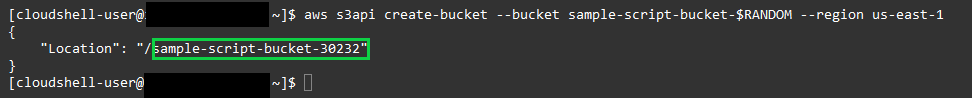
• We begin by creating an S3 bucket where we store the script for our AWS Glue streaming job. Run the following command in your terminal to create a new bucket:

aws s3api create-bucket --bucket sample-script-bucket-$RANDOM --region us-east-1

• Note down the name of the bucket created.

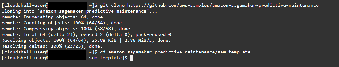
• Next, we clone the code repository locally, which contains the CloudFormation template to deploy the stack. Run the following command in your terminal:

git clone https://github.com/aws-samples/amazon-sagemaker-predictive-maintenance

• Navigate to the sam-template directory:

cd amazon-sagemaker-predictive-maintenance/sam-template

• Run the following command to copy the AWS Glue job script (from glue_streaming/app.py) to the S3 bucket you created:

aws s3 cp glue_streaming/app.py s3://sample-script-bucket-30232/glue_streaming/app.py

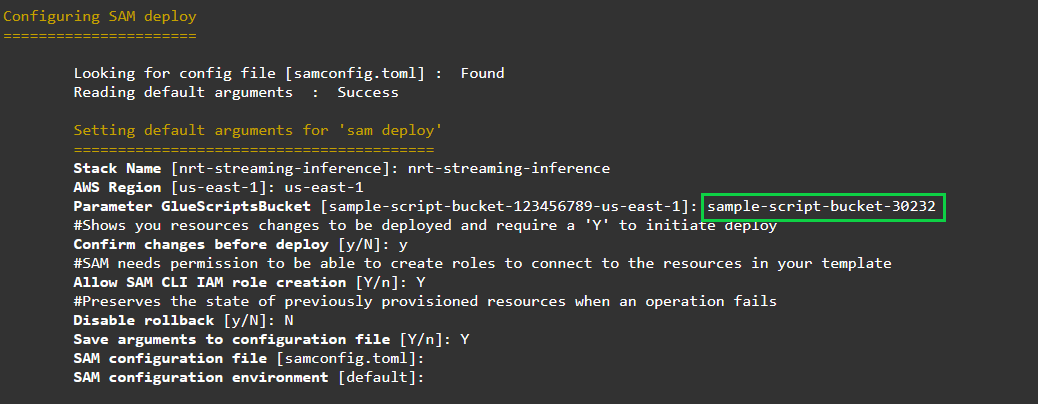
• You can now go ahead with the build and deployment of the solution, through the CloudFormation template via AWS SAM. Run the following command:

sam build

sam deploy --guided

• Provide arguments for the deployment such as the stack name, preferred AWS Region (us-east-1), and GlueScriptsBucket.

Make sure you provide the same S3 bucket that you created earlier for the AWS Glue script S3 bucket (parameter GlueScriptsBucket in the following screenshot).

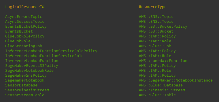
After you provide the required arguments, AWS SAM starts the stack deployment. The following screenshot shows the resources created.

After the stack is deployed successfully, you should see the following message.

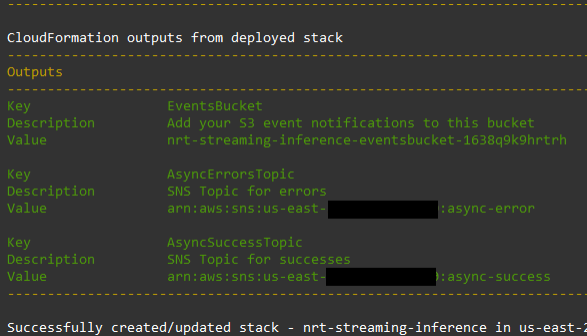
• On the AWS CloudFormation console, open the stack (for this post, nrt-streaming-inference) that was provided when deploying the CloudFormation template.
• On the Resources tab, note the SageMaker notebook instance ID.

• On the SageMaker console, open this instance.

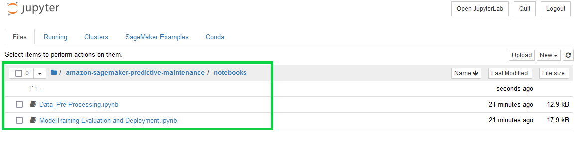
The SageMaker notebook instance already has the required notebooks pre-loaded.

Navigate to the notebooks folder and open and follow the instructions within the notebooks (Data_Pre-Processing.ipynb and ModelTraining-Evaluation-and-Deployment.ipynb) to explore the dataset, perform preprocessing and feature engineering, and train and deploy the model to a SageMaker asynchronous inference endpoint.

Streaming data source and ingestion

Kinesis Data Streams is a serverless, scalable, and durable real-time data streaming service that you can use to collect and process large streams of data records in real time. Kinesis Data Streams enables capturing, processing, and storing data streams from a variety of sources, such as IT infrastructure log data, application logs, social media, market data feeds, web clickstream data, IoT devices and sensors, and more. You can provision a Kinesis data stream in on-demand mode or provisioned mode depending on the throughput and scaling requirements. For more information, see Choosing the Data Stream Capacity Mode.

For our use case, we assume that various sensors are sending measurements such as temperature, rotation speed, torque, and tool wear to a data stream. Kinesis Data Streams acts as a funnel to collect and ingest data streams.

We use the Amazon Kinesis Data Generator (KDG) later in this post to generate and send data to a Kinesis data stream, simulating data being generated by sensors. The data from the data stream sensor-data-stream is ingested and processed using an AWS Glue streaming job, which we discuss next.

Near-real-time feature engineering

AWS Glue streaming jobs provide a convenient way to process streaming data at scale, without the need to manage the compute environment. AWS Glue allows you to perform extract, transform, and load (ETL) operations on streaming data using continuously running jobs. AWS Glue streaming ETL is built on the Apache Spark Structured Streaming engine, and can ingest streams from Kinesis, Apache Kafka, and Amazon Managed Streaming for Apache Kafka (Amazon MSK).

The streaming ETL job can use both AWS Glue built-in transforms and transforms that are native to Apache Spark Structured Streaming. You can also use the Spark ML and MLLib libraries in AWS Glue jobs for easier feature processing using readily available helper libraries.

If the schema of the streaming data source is pre-determined, you can specify it in an AWS Data Catalog table. If the schema definition can’t be determined beforehand, you can enable schema detection in the streaming ETL job. The job then automatically determines the schema from the incoming data. Additionally, you can use the AWS Glue Schema Registry to allow central discovery, control, and evolution of data stream schemas. You can further integrate the Schema Registry with the Data Catalog to optionally use schemas stored in the Schema Registry when creating or updating AWS Glue tables or partitions in the Data Catalog.

For this post, we create an AWS Glue Data Catalog table (sensor-stream) with our Kinesis data stream as the source and define the schema for our sensor data.

We create an AWS Glue dynamic dataframe from the Data Catalog table to read the streaming data from Kinesis. We also specify the following options:

• A window size of 60 seconds, so that the AWS Glue job reads and processes data in 60-second windows
• The starting position TRIM_HORIZON, to allow reading from the oldest records in the Kinesis data stream

We also use Spark MLlib’s StringIndexer feature transformer to encode the string column type into label indexes. This transformation is implemented using Spark ML Pipelines. Spark ML Pipelines provide a uniform set of high-level APIs for ML algorithms to make it easier to combine multiple algorithms into a single pipeline or workflow.

We use the foreachBatch API to invoke a function named processBatch, which in turn processes the data referenced by this dataframe. See the following code:

# Read from Kinesis Data Stream
sourceStreamData = glueContext.create_data_frame.from_catalog(database = "sensordb", table_name = "sensor-stream", transformation_ctx = "sourceStreamData", additional_options = {"startingPosition": "TRIM_HORIZON"})
type_indexer = StringIndexer(inputCol="type", outputCol="type_enc", stringOrderType="alphabetAsc")
pipeline = Pipeline(stages=[type_indexer])
glueContext.forEachBatch(frame = sourceStreamData, batch_function = processBatch, options = {"windowSize": "60 seconds", "checkpointLocation": checkpoint_location})

The function processBatch performs the specified transformations and partitions the data in Amazon S3 based on year, month, day, and batch ID.

We also re-partition the AWS Glue partitions into a single partition, to avoid having too many small files in Amazon S3. Having several small files can impede read performance, because it amplifies the overhead related to seeking, opening, and reading each file. We finally write the features to generate inferences into a prefix (features) within the S3 bucket. See the following code:

# Function that gets called to perform processing, feature engineering and writes to S3 for every micro batch of streaming data from Kinesis.
def processBatch(data_frame, batchId):
transformer = pipeline.fit(data_frame)
now = datetime.datetime.now()
year = now.year
month = now.month
day = now.day
hour = now.hour
minute = now.minute
if (data_frame.count() > 0):
data_frame = transformer.transform(data_frame)
data_frame = data_frame.drop("type")
data_frame = DynamicFrame.fromDF(data_frame, glueContext, "from_data_frame")
data_frame.printSchema()
# Write output features to S3
s3prefix = "features" + "/year=" + "{:0>4}".format(str(year)) + "/month=" + "{:0>2}".format(str(month)) + "/day=" + "{:0>2}".format(str(day)) + "/hour=" + "{:0>2}".format(str(hour)) + "/min=" + "{:0>2}".format(str(minute)) + "/batchid=" + str(batchId)
s3path = "s3://" + out_bucket_name + "/" + s3prefix + "/"
print("-------write start time------------")
print(str(datetime.datetime.now()))
data_frame = data_frame.toDF().repartition(1)
data_frame.write.mode("overwrite").option("header",False).csv(s3path)
print("-------write end time------------")
print(str(datetime.datetime.now()))

Model training and deployment

SageMaker is a fully managed and integrated ML service that enables data scientists and ML engineers to quickly and easily build, train, and deploy ML models.

Within the Data_Pre-Processing.ipynb notebook, we first import the AI4I Predictive Maintenance dataset from the UCI Data Repository and perform exploratory data analysis (EDA). We also perform feature engineering to make our features more useful for training the model.

For example, within the dataset, we have a feature named type, which represents the product’s quality type as L (low), M (medium), or H (high). Because this is categorical feature, we need to encode it before training our model. We use Scikit-Learn’s LabelEncoder to achieve this:

from sklearn.preprocessing import LabelEncoder
type_encoder = LabelEncoder()
type_encoder.fit(origdf['type'])
type_values = type_encoder.transform(origdf['type'])

After the features are processed and the curated train and test datasets are generated, we’re ready to train an ML model to predict whether the machine failed or not based on system readings. We train a XGBoost model, using the SageMaker built-in algorithm. XGBoost can provide good results for multiple types of ML problems, including classification, even when training samples are limited.

SageMaker training jobs provide a powerful and flexible way to train ML models on SageMaker. SageMaker manages the underlying compute infrastructure and provides multiple options to choose from, for diverse model training requirements, based on the use case.

xgb = sagemaker.estimator.Estimator(container,
role,
instance_count=1,
instance_type='ml.c4.4xlarge',
output_path=xgb_upload_location,
sagemaker_session=sagemaker_session)
xgb.set_hyperparameters(max_depth=5,
eta=0.2,
gamma=4,
min_child_weight=6,
subsample=0.8,
silent=0,
objective='binary:hinge',
num_round=100)

xgb.fit({'train': s3_train_channel, 'validation': s3_valid_channel})

When the model training is complete and the model evaluation is satisfactory based on the business requirements, we can begin model deployment. We first create an endpoint configuration with the AsyncInferenceConfig object option and using the model trained earlier:

endpoint_config_name = resource_name.format("EndpointConfig")
create_endpoint_config_response = sm_client.create_endpoint_config(
EndpointConfigName=endpoint_config_name,
ProductionVariants=[
{
"VariantName": "variant1",
"ModelName": model_name,
"InstanceType": "ml.m5.xlarge",
"InitialInstanceCount": 1,
}
],
AsyncInferenceConfig={
"OutputConfig": {
"S3OutputPath": f"s3://{bucket}/{prefix}/output",
#Specify Amazon SNS topics
"NotificationConfig": {
"SuccessTopic": "arn:aws:sns:<region>:<account-id>:<success-sns-topic>",
"ErrorTopic": "arn:aws:sns:<region>:<account-id>:<error-sns-topic>",
}},
"ClientConfig": {"MaxConcurrentInvocationsPerInstance": 4},
},)

We then create a SageMaker asynchronous inference endpoint, using the endpoint configuration we created. After it’s provisioned, we can start invoking the endpoint to generate inferences asynchronously.

endpoint_name = resource_name.format("Endpoint")
create_endpoint_response = sm_client.create_endpoint(
EndpointName=endpoint_name, EndpointConfigName=endpoint_config_name)

Near-real-time inference

SageMaker asynchronous inference endpoints provide the ability to queue incoming inference requests and process them asynchronously in near-real time. This is ideal for applications that have inference requests with larger payload sizes (up to 1 GB), may require longer processing times (up to 15 minutes), and have near-real-time latency requirements. Asynchronous inference also enables you to save on costs by auto scaling the instance count to zero when there are no requests to process, so you only pay when your endpoint is processing requests.

You can create a SageMaker asynchronous inference endpoint similar to how you create a real-time inference endpoint and additionally specify the AsyncInferenceConfig object, while creating your endpoint configuration with the EndpointConfig field in the CreateEndpointConfig API. The following diagram shows the inference workflow and how an asynchronous inference endpoint generates an inference.

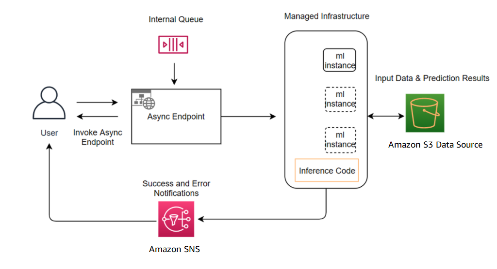
To invoke the asynchronous inference endpoint, the request payload should be stored in Amazon S3 and reference to this payload needs to be provided as part of the InvokeEndpointAsync request. Upon invocation, SageMaker queues the request for processing and returns an identifier and output location as a response. Upon processing, SageMaker places the result in the Amazon S3 location. You can optionally choose to receive success or error notifications with Amazon Simple Notification Service (Amazon SNS).

Test the end-to-end solution

To test the solution, complete the following steps:

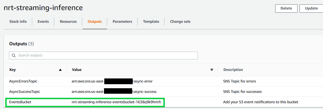
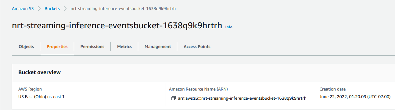
• On the AWS CloudFormation console, open the stack you created earlier (nrt-streaming-inference).
• On the Outputs tab, copy the name of the S3 bucket (EventsBucket).

This is the S3 bucket to which our AWS Glue streaming job writes features after reading and processing from the Kinesis data stream.

Next, we set up event notifications for this S3 bucket.

• On the Amazon S3 console, navigate to the bucket EventsBucket.
• On the Properties tab, in the Event notifications section, choose Create event notification.

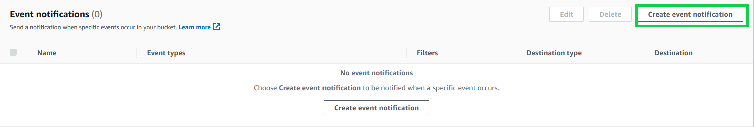
• For Event name, enter invoke-endpoint-lambda.
• For Prefix, enter features/.
• For Suffix, enter .csv.
• For Event types, select All object create events.

• For Destination, select Lambda function.
• For Lambda function, and choose the function invoke-endpoint-asynch.
• Choose Save changes.

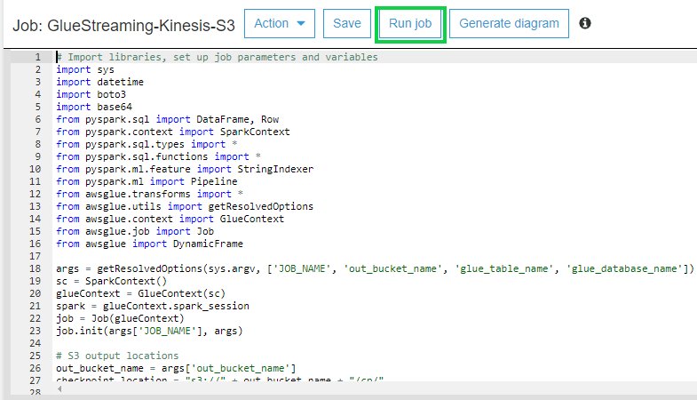
• On the AWS Glue console, open the job GlueStreaming-Kinesis-S3.
• Choose Run job.

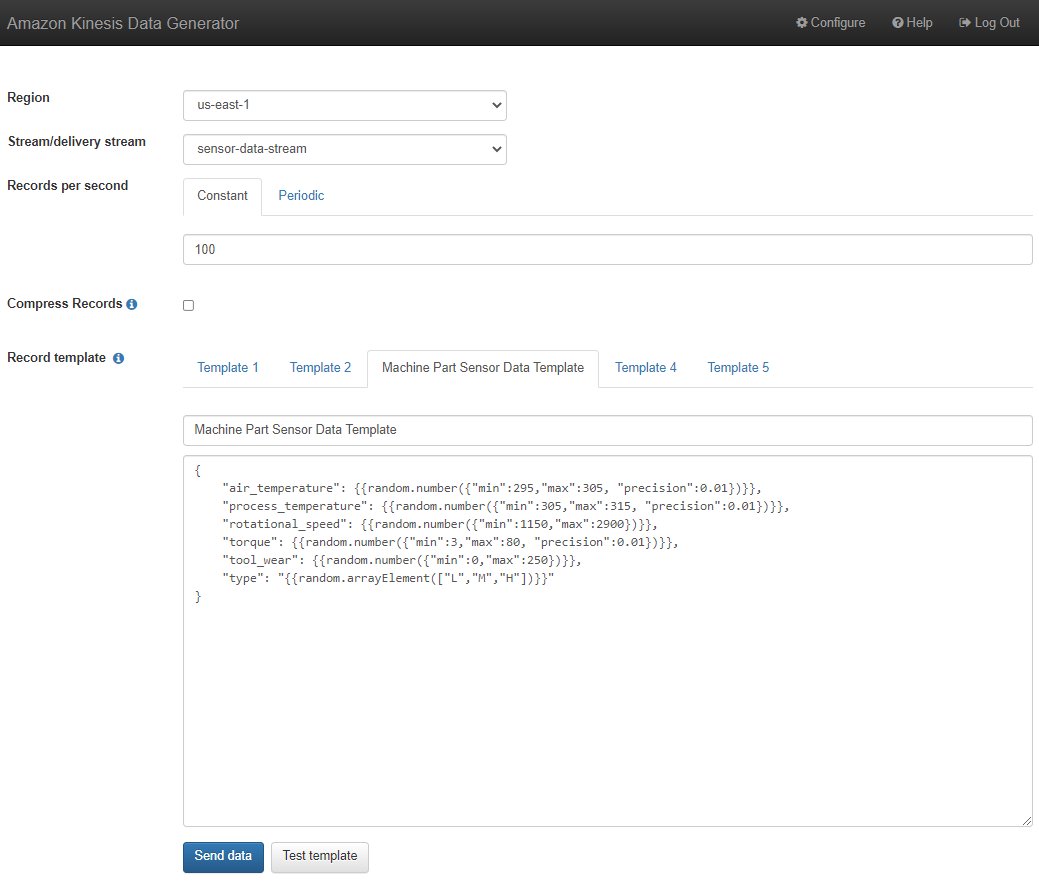
Next we use the Kinesis Data Generator (KDG) to simulate sensors sending data to our Kinesis data stream. If this is your first time using the KDG, refer to Overview for the initial setup. The KDG provides a CloudFormation template to create the user and assign just enough permissions to use the KDG for sending events to Kinesis. Run the CloudFormation template within the AWS account that you’re using to build the solution in this post. After the KDG is set up, log in and access the KDG to send test events to our Kinesis data stream.

• Use the Region in which you created the Kinesis data stream (us-east-1).
• On the drop-down menu, choose the data stream sensor-data-stream.
• In the Records per second section, select Constant and enter 100.
• Unselect Compress Records.
• For Record template, use the following template:

{
"air_temperature": {{random.number({"min":295,"max":305, "precision":0.01})}},
"process_temperature": {{random.number({"min":305,"max":315, "precision":0.01})}},
"rotational_speed": {{random.number({"min":1150,"max":2900})}},
"torque": {{random.number({"min":3,"max":80, "precision":0.01})}},
"tool_wear": {{random.number({"min":0,"max":250})}},
"type": "{{random.arrayElement(["L","M","H"])}}"
}

• Click Send data to start sending data to the Kinesis data stream.

The AWS Glue streaming job reads and extracts a micro-batch of data (representing sensor readings) from the Kinesis data stream based on the window size provided. The streaming job then processes and performs feature engineering on this micro-batch before partitioning and writing it to the prefix features within the S3 bucket.

As new features created by the AWS Glue streaming job are written to the S3 bucket, a Lambda function (invoke-endpoint-asynch) is triggered, which invokes a SageMaker asynchronous inference endpoint by sending an invocation request to get inferences from our deployed ML model. The asynchronous inference endpoint queues the request for asynchronous invocation. When the processing is complete, SageMaker stores the inference results in the Amazon S3 location (S3OutputPath) that was specified during the asynchronous inference endpoint configuration.

For our use case, the inference results indicate if a machine part is likely to fail or not, based on the sensor readings.

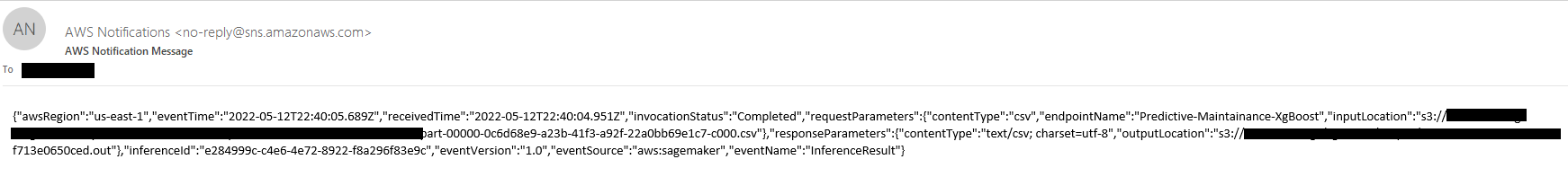
SageMaker also sends a success or error notification with Amazon SNS. For example, if you set up an email subscription for the success and error SNS topics (specified within the asynchronous SageMaker inference endpoint configuration), an email can be sent every time an inference request is processed. The following screenshot shows a sample email from the SNS success topic.

For real-world applications, you can integrate SNS notifications with other services such as Amazon Simple Queue Service (Amazon SQS) and Lambda for additional postprocessing of the generated inferences or integration with other downstream applications, based on your requirements. For example, for our predictive maintenance use case, you can invoke a Lambda function based on an SNS notification to read the generated inference from Amazon S3, further process it (such as aggregation or filtering), and initiate workflows such as sending work orders for equipment repair to technicians.

Clean up

When you’re done testing the stack, delete the resources (especially the Kinesis data stream, Glue streaming job, and SNS topics) to avoid unexpected charges.

Run the following code to delete your stack:

sam delete nrt-streaming-inference

Also delete the resources such as SageMaker endpoints by following the cleanup section in the ModelTraining-Evaluation-and-Deployment notebook.

Conclusion

In this post, we used a predictive maintenance use case to demonstrate how to use various services such as Kinesis, AWS Glue, and SageMaker to build a near-real-time inference pipeline. We encourage you to try this solution and let us know what you think.

If you have any questions, share them in the comments.

About the authors

Rahul Sharma is a Solutions Architect at AWS Data Lab, helping AWS customers design and build AI/ML solutions. Prior to joining AWS, Rahul has spent several years in the finance and insurance sector, helping customers build data and analytical platforms.

Pat Reilly is an Architect in the AWS Data Lab, where he helps customers design and build data workloads to support their business. Prior to AWS, Pat consulted at an AWS Partner, building AWS data workloads across a variety of industries.

Read More

LiDAR is a key enabling technology in growing autonomous markets, such as robotics, industrial, infrastructure, and automotive. LiDAR delivers precise 3D data about its environment in real time to provide “vision” for autonomous solutions. For autonomous vehicles (AVs), nearly every carmaker uses LiDAR to augment camera and radar systems for a comprehensive perception stack capable of safely navigating complex roadway environments. Computer vision systems can use the 3D maps generated by LiDAR sensors for object detection, object classification, and scene segmentation. Like any other supervised machine learning (ML) system, the point cloud data generated by LiDAR sensors should be labeled correctly in order for the ML model to make correct inferences. This allows AVs to operate smoothly and efficiently, avoiding incidents and collisions with objects, pedestrians, vehicles, and other road users.

In this post, we demonstrate how to label 3D point cloud data generated by Velodyne LiDAR sensors using Amazon SageMaker Ground Truth. We break down the process of sending data for annotation so that you can obtain precise, high-quality results.

The code for this example is available on GitHub.

Solution overview

SageMaker Ground Truth is a data labeling service that you can use to create high-quality labeled datasets for various types of ML use cases. SageMaker Ground Truth is a capability in Amazon SageMaker, which is a comprehensive and fully managed ML service. With SageMaker, data scientists and developers can quickly and easily build and train ML models, and then directly deploy them into a production-ready environment.

In addition to LiDAR data, we also include camera images, using the sensor fusion feature in SageMaker Ground Truth to deliver robust visual information about the scenes that annotators are labeling. Through sensor fusion, annotators can adjust labels in the 3D scene as well as in 2D images. It delivers the unique capability to ensure that annotations in LiDAR data are mirrored in 2D imagery, making the process more efficient.

With SageMaker Ground Truth, Velodyne LiDAR’s 3D point cloud data generated by a Velodyne LiDAR sensor mounted on a vehicle can be labeled for tracking moving objects. In this challenging use case, we can follow the trajectory of an object like a car or a pedestrian in a dynamic environment, while our point of reference is also moving. In this case, our point of reference is a car that is equipped with Velodyne LiDAR.

To perform this task, we walk through the following topics:

• Velodyne technology
• The dataset
• Creating a labeling job
• The point cloud sequence input manifest file
• Building the sequence input manifest file
• Labeling the category configuration file
• Specifying the job resources
• Completing a labeling job

Prerequisites

To implement the solution in this post, you must have the following prerequisites:

• An AWS account for running the code.
• An Amazon Simple Storage Service (Amazon S3) bucket you can write to. The bucket must be in the same Region as the SageMaker notebook instance. We can also define a valid S3 prefix. All the files related to this experiment are stored in that prefix of our bucket. We must attach the CORS policy to this bucket. For instructions, refer to Configuring cross-origin resource sharing (CORS). Enter the following policy in the CORS configuration editor:

<?xml version="1.0" encoding="UTF-8"?>
<CORSConfiguration xmlns="http://s3.amazonaws.com/doc/2006-03-01/">
<CORSRule>
    <AllowedOrigin>*</AllowedOrigin>
    <AllowedMethod>GET</AllowedMethod>
    <AllowedMethod>HEAD</AllowedMethod>
    <AllowedMethod>PUT</AllowedMethod>
    <MaxAgeSeconds>3000</MaxAgeSeconds>
    <ExposeHeader>Access-Control-Allow-Origin</ExposeHeader>
    <AllowedHeader>*</AllowedHeader>
</CORSRule>
<CORSRule>
    <AllowedOrigin>*</AllowedOrigin>
    <AllowedMethod>GET</AllowedMethod>
</CORSRule>
</CORSConfiguration>

• An AWS Identity and Access Management (IAM) role to access SageMaker.
• A SageMaker notebook instance.
• Familiarity with the Ground Truth 3D point cloud labeling job.
• Familiarity with Python and NumPy.
• Basic understanding of SageMaker.
• Basic familiarity with the AWS Command Line Interface (AWS CLI).
• The code and associated dataset.

Velodyne technology

LiDAR can be divided into different categories, including scanning LiDAR and flash LiDAR. Conventionally scanning LiDAR uses mechanical rotation to spin the sensor for 360-degree detection. Velodyne, which invented the industry’s first 3D LiDAR, continues to innovate and launch new rotational products with cutting-edge technology. Velodyne’s Ultra Puck is a scanning LiDAR sensor that uses Velodyne’s patented surround view technology. It provides a full 360-degree environmental view to deliver accurate real-time 3D data. The Ultra Puck has a compact form factor and delivers the real-time object detection needed for safe navigation and reliable operation. With a combination of optimal power and high performance, this sensor provides distance and calibrated reflectivity measurements at all rotational angles. It’s an ideal solution for robotics, mapping, security, driver assistance, and autonomous navigation. Besides the LiDAR sensor itself, Velodyne has created the Vella Development Kit (VDK), a collection of tools, hardware, and documentation that facilitate access to the Velodyne’s autonomy software stack. The VDK can be configured for different custom interfaces and environments, providing you with a broad range of applications for increased autonomy and improved safety.

Additionally, the VDK can reduce the upfront work you would have to otherwise put in to enable an end-to-end data collection and annotation pipeline by providing the following necessary capabilities:

• Clock synchronization between LiDAR, odometry, and camera frames
• Calibration for LiDAR vehicle 5-DOF extrinsic calibration (z is not observable)
• Calibration for LiDAR camera extrinsic, intrinsic, and distortion parameters
• Collect motion compensated (intra-frame or multi-frame), synchronized LiDAR point clouds and camera images

To develop vehicle-based perception capabilities, Velodyne’s software team has set up their own data collection vehicle with one of their Ultra Puck LiDAR units, a camera and GPS/IMU sensors mounted to the vehicle hood. In the subsequent steps, we refer to their internal processes that use the VDK to prepare, collect, and annotate data needed to develop their vehicle-based perception capabilities as an example to other customers trying to solve their own perception use cases.

Clock synchronization

Accurate clock synchronization of the LiDAR, odometry, and camera outputs can be crucial for any multi-sensor application that combines those data streams. For best results, you should use a PTP synchronization system with a primary clock and support by all sensors. One advantage of PTP is the ability to synchronize multiple devices to high accuracy with a single timing source. Such a system can achieve synchronization accuracy better than 1 microsecond. Other solutions include PPS distribution and per-device time sources. As an alternative option, the VDK supports software synchronization utilizing time-of-arrival timestamping, which can be a great way to get an application off the ground quickly in the absence of proper clock synchronization infrastructure. This can result in timestamping errors on the order of 1–10 milliseconds due to a combination of latency and queuing delays at various levels of the network infrastructure and host operating system, which may or may not be acceptable, depending on the application.

LiDAR vehicle calibration

The LiDAR vehicle calibration estimates the extrinsic position of the LiDAR in vehicle frame along five axes. Z value is unobservable; therefore you must measure the z value independently. Our process is a targetless calibration technique but it works well in an environment where the ground is relatively flat, and the environment has contiguous static objects features rather than dynamic (vehicles, pedestrians) or non-contiguous (shrubs and bushes) features. Think of a parking lot with few obstacles and buildings with flat facades. The presence of geometric structures is ideal for improving the calibration quality. The user is required to drive in some predefined driving patterns indicated by the VDK to expose most of the parameters. One minute of data is sufficient for this calibration. After the data is uploaded to Veldoyne’s platform service, the calibration takes place on the cloud and the result is made available within 24 hours. For the purposes of this notebook, the calibration parameters have already been processed and provided.

The LiDAR dataset

The dataset and resources used in this notebook are provided by Velodyne. This dataset contains one continuous scene from an autonomous vehicle experiment driving around on a highway in California. The entire scene contains 60 frames. The dataset contents are as follows:

• lidar_cam_calib_vlp32_06_10_2021.yaml – Camera calibration information, one camera only
• images/ – Camera footage for each frame
• poses/ – Pose JSON file containing LiDAR extrinsic matrix for each frame
• rectified_scans_local/ – .pcb files in LiDAR sensor local coordinate system

Run the following code to download the dataset locally and then upload to your S3 bucket, which we defined in the initialization section:

source_bucket = 'velodyne-blog'
source_prefix = 'highway_data_07'
source_data = f's3://{source_bucket}/{source_prefix}'

!aws s3 cp $source_data ./$PREFIX --recursive
target_s3 = f's3://{BUCKET}/{PREFIX}'
!aws s3 cp ./$PREFIX $target_s3 –recursive

Create a labeling job

As the next step, we need to create a data labeling job in SageMaker Ground Truth. We select the task type as object tracking. For more information about 3D point cloud labeling task types, refer to 3D Point Cloud Task types. To create an object tracking point cloud labeling job, we need to add the following resources as the labeling job inputs:

• Point cloud sequence input manifest – A JSON file defining the point cloud frame sequence and associated sensor fusion data. For more information, see Create a Point Cloud Sequence Input Manifest.
• Input manifest file – The input file for the labeling job. Each line of the manifest file contains a link to a sequence file defined in the point cloud sequence input manifest.
• Label category configuration file – This file is used to specify your labels, label category, frame attributes, and worker instructions. For more information, see Create a Labeling Category Configuration File with Label Category and Frame Attributes.
• Predefined AWS resources – Includes the following:
  • Pre-annotation Lambda ARN – Refer to PreHumanTaskLambdaArn.
  • Annotation consolidation ARN – The AWS Lambda function used to consolidate labels from different workers. Refer to AnnotationConsolidationLambdaArn.
  • Workforce ARN – Defines which workforce type we want to use. Refer to Create and Manage Workforces for more details.
  • HumanTaskUiArn – Defines the worker UI template to do the labeling job. This should have a format similar to arn:aws:sagemaker:<region>:123456789012:human-task-ui/PointCloudObjectTracking.

Keep in mind the following:

• There should not be an entry for the UiTemplateS3Uri parameter.
• Your LabelAttributeName must end in -ref. For example, ot-labels-ref.
• The number of workers specified in NumberOfHumanWorkersPerDataObject should be 1.
• 3D point cloud labeling doesn’t support active learning, so we shouldn’t specify values for parameters in LabelingJobAlgorithmsConfig.
• 3D point cloud object tracking labeling jobs can take multiple hours to complete. You should specify a longer time limit for these labeling jobs in TaskTimeLimitInSeconds (up to 7 days, or 604,800 seconds).

  #object tracking as our 3D Point Cloud Task Type. 
  task_type = "3DPointCloudObjectTracking"

Point cloud sequence input manifest file

The following of the most important steps to generating a sequence input manifest file:

1. Convert the 3D points to a world coordinate system.
2. Generate the sensor extrinsic matrix to enable the sensor fusion feature in SageMaker Ground Truth.

The LiDAR sensor is mounted on a moving vehicle (ego vehicle), which captures the data in its own frame of reference. To perform object tracking, we need to convert this data to a global frame of reference to account for the moving ego vehicle itself. This is the world coordinate system.

Sensor fusion is a feature in SageMaker Ground Truth that synchronizes the 3D point cloud frame side by side with the camera frame. This provides visual context for human labelers and allows labelers to adjust annotation in 3D and 2D images synchronously. For instructions on matrix transformation, refer to Labeling data for 3D object tracking and sensor fusion in Amazon SageMaker Ground Truth.

The generate_transformed_pcd_from_point_cloud function performs the coordinate translation and then generates the 3D point data file, which SageMaker Ground Truth can consume.

To translate the data from local/sensor global coordinate system, multiply each point in a 3D frame with the extrinsic matrix for the LiDAR sensor.

SageMaker Ground Truth renders the 3D point cloud data in either Compact Binary Pack (.bin) or ASCII (.txt) format. Files in these formats need to contain information about the location (x, y, and z coordinates) of all points that make up that frame, and, optionally, information about the pixel color of each point for colored point clouds (i, r, g, b).

To read more about SageMaker Ground Truth accepted raw 3D data formats, see Accepted Raw 3D Data Formats.

Build the sequence input manifest file

The next step is to build the point cloud sequence input manifest file. The steps listed in this section are also available in the notebook.

1. Point the cloud data from the .pcd file, the LiDAR extrinsic matrix from the pose file, and the camera extrinsic, intrinsic, and distortion data from the camera calibration .yaml file.
2. Perform a per-frame transform of the raw point cloud to the global frame of reference. Generate and store ASCII (.txt) for each frame to Amazon S3.
3. Extract the ego vehicle pose from the LiDAR extrinsic matrix.
4. Build a sensor position in the global coordinate system by extracting the camera pose from the camera inverse extrinsic matrix.
5. Provide camera calibration parameters (such as distortion and skew).
6. Build the array of data frames. Reference the ASCII file location, define the vehicle position in world coordinate system, and so on.
7. Create the sequence manifest file sequence.json.
8. Create our input manifest file. Each line identifies a single sequence file we just uploaded.

Label the category configuration file

Our label category configuration file is used to specify labels, or classes, for our labeling job. When we use the object detection or object tracking task types; we can also include label attributes in our label category configuration file. Workers can assign one or more attributes we provide to annotations to give more information about that object. For example, we may want to use the attribute occluded to have workers identify when an object is partially obstructed. Let’s look at an example of the label category configuration file for an object detection or object tracking labeling job:

label_category = {
  "categoryGlobalAttributes": [
    {
      "enum": [
        "75-100%",
        "25-75%",
        "0-25%"
      ],
      "name": "Visibility",
      "type": "string"
    }
  ],
  "documentVersion": "2020-03-01",
  "instructions": {
    "fullInstruction": "Draw a tight Cuboid. You only need to annotate those in the first frame. Please make sure the direction of the cubiod is accurately representative of the direction of the vehicle it bounds.",
    "shortInstruction": "Draw a tight Cuboid. You only need to annotate those in the first frame."
  },
  "labels": [
    {
      "categoryAttributes": [],
      "label": "Car"
    },
    {
      "categoryAttributes": [],
      "label": "Truck"
    },
    {
      "categoryAttributes": [],
      "label": "Bus"
    },
    {
      "categoryAttributes": [],
      "label": "Pedestrian"
    },
    {
      "categoryAttributes": [],
      "label": "Cyclist"
    },
    {
      "categoryAttributes": [],
      "label": "Motorcyclist"
    },
  ]
}

category_key = f'{PREFIX}/manifests_categories/label_category.json'
write_json_to_s3(label_category, BUCKET, category_key)

label_category_file = f's3://{BUCKET}/{category_key}'
print(f"label category file uri: {label_category_file}")

Specify the job resources

As the next step, we specify various labeling job resources:

• Human task UI ARN – HumanTaskUiArn is a resource that defines the worker task template used to render the worker UI and tools for the labeling job. This attribute is defined under UiConfig and the resource name is configured by Region and task type:

  human_task_ui_arn = (
      f"arn:aws:sagemaker:{region}:123456789012:human-task-ui/{task_type[2:]}"
  )

• Work resource – In this example, we use private team resources. For instructions, refer to Create a Private Workforce (Amazon Cognito Console). When we’re done, we should put our resource ARN in the following parameter:

  workteam_arn = f"arn:aws:sagemaker:{region}:123456789012:workteam/private-crowd/test-team"#"<REPLACE W/ YOUR Private Team ARN>"

• Pre-annotation Lambda ARN and post-annotation Lambda ARN – See the following code:

  ac_arn_map = {
      "us-west-2": "081040173940",
      "us-east-1": "432418664414",
      "us-east-2": "266458841044",
      "eu-west-1": "568282634449",
      "ap-northeast-1": "477331159723",
  }
  
  prehuman_arn = "arn:aws:lambda:{}:{}:function:PRE-{}".format(region, ac_arn_map[region], task_type)
  acs_arn = "arn:aws:lambda:{}:{}:function:ACS-{}".format(region, ac_arn_map[region], task_type)

• HumanTaskConfig – We use this to specify our work team and configure our labeling job task. Feel free to update the task description in the following code:

  job_name = f"velodyne-blog-test-{str(time.time()).split('.')[0]}"
  
  # Task description info =================
  task_description = "Draw 3D boxes around required objects"
  task_keywords = ['lidar', 'pointcloud']
  task_title = job_name
  
  human_task_config = {
      "AnnotationConsolidationConfig": {
          "AnnotationConsolidationLambdaArn": acs_arn,
      },
      "WorkteamArn": workteam_arn,
      "PreHumanTaskLambdaArn": prehuman_arn,
      "MaxConcurrentTaskCount": 200,
      "NumberOfHumanWorkersPerDataObject": 1,  # One worker will work on each task
      "TaskAvailabilityLifetimeInSeconds": 18000, # Your workteam has 5 hours to complete all pending tasks.
      "TaskDescription": task_description,
      "TaskKeywords": task_keywords,
      "TaskTimeLimitInSeconds": 36000, # Each seq must be labeled within 1 hour.
      "TaskTitle": task_title,
      "UiConfig": {
          "HumanTaskUiArn": human_task_ui_arn,
      },
  }

Create the labeling job

Next, we create the labeling request, as shown in the following code:

labelAttributeName = f"{job_name}-ref" #must end with -ref

output_path = f"s3://{BUCKET}/{PREFIX}/output"

ground_truth_request = {
    "InputConfig" : {
      "DataSource": {
        "S3DataSource": {
          "ManifestS3Uri": manifest_uri,
        }
      },
      "DataAttributes": {
        "ContentClassifiers": [
          "FreeOfPersonallyIdentifiableInformation",
          "FreeOfAdultContent"
        ]
      },  
    },
    "OutputConfig" : {
      "S3OutputPath": output_path,
    },
    "HumanTaskConfig" : human_task_config,
    "LabelingJobName": job_name,
    "RoleArn": role, 
    "LabelAttributeName": labelAttributeName,
    "LabelCategoryConfigS3Uri": label_category_file,
    "Tags": [],
}

Finally, we create the labeling job:

sagemaker_client.create_labeling_job(**ground_truth_request)

Complete a labeling job

When our labeling job is ready, we can add ourselves to our private work team and experiment with the worker’s portal. We should receive an email with the portal link, our user name, and a temporary password. When we log in, we choose the labeling job from the list, and then we should see the worker’s portal like the following screenshot. (It may take a few minutes for a new labeling job to show up in the portal). More information on how to set up workers and instructions can be found here and here respectively.

When we’re are done with the labeling job, we can choose Submit, and then view the output data in the S3 output location we specified earlier.

Conclusion

In this post, we showed how we can create a 3D point cloud labeling job for object tracking for data captured using Velodyne’s LiDAR sensor. We followed the step-by-step instructions in this post and ran the provided code to create a SageMaker Ground Truth labeling job to label the 3D point cloud data. ML models can use the labels created with this job to train object detection, object recognition, and object tracking models commonly used in autonomous vehicle scenarios.

If you are interested in labeling 3D point cloud data captured via Velodyne’s LiDAR sensor, follow the steps in this article to label the data using Amazon SageMaker Ground Truth.

About the Authors

Sharath Nair leads the Computer Vision team that focusses on building perception algorithms for some of Velodyne’s software products like Object Detection & Tracking, Semantic Segmentation, SLAM, etc. Prior to Velodyne, Sharath worked on Autonomous Vehicles and Robotics and has been involved in this space for the past 6 years.

Oliver Monson is a Senior Data Operations Manager at Velodyne Lidar, responsible for the data pipelines and acquisition strategies that support the development of perception software. Prior to Velodyne, Oliver has managed operational teams executing on HD mapping, geospatial, and archaeological applications.

John Kua is Director of Software Engineering at Velodyne, overseeing the System Integration and Robotics, Vella Go, and Software Production teams. Prior to joining Velodyne, John spent over a decade building multimodal sensor platforms for a wide range of 3D localization and mapping applications in commercial and government applications. These platforms included a wide array of sensors including visible light, thermal, and hyperspectral cameras, lidar, GPS, IMUs, and even gamma-ray spectrometers and imagers.

Sally Frykman, Chief Marketing Officer at Velodyne, oversees the strategic development and execution of global marketing and communications programs that advance the company’s innovative vision and goals. Her multifaceted role encompasses a wide array of responsibilities, including promotion of the Velodyne brand, thought leadership development, and robust sales lead generation fueled by highly engaging digital marketing. Previously, Sally worked in public education and social work.

Nitin Wagh is Sr. Business Development Manager for Amazon AI. He likes the opportunity to help customers understand Machine Learning and  power of Augmented AI in AWS cloud. In his spare time, he loves spending time with family in outdoors activities.

James Wu is a Senior AI/ML Specialist Solution Architect at AWS. helping customers design and build AI/ML solutions. James’s work covers a wide range of ML use cases, with a primary interest in computer vision, deep learning, and scaling ML across the enterprise. Prior to joining AWS, James was an architect, developer, and technology leader for over 10 years, including 6 years in engineering and 4 years in marketing & advertising industries.

Farooq Sabir is a Senior Artificial Intelligence and Machine Learning Specialist Solutions Architect at AWS. He holds PhD and MS degrees in Electrical Engineering from The University of Texas at Austin and a MS in Computer Science from Georgia Institute of Technology. He has over 15 years of work experience and also likes to teach and mentor college students. At AWS, he helps customers formulate and solve their business problems in data science, machine learning, computer vision, artificial intelligence, numerical optimization and related domains. Based in Dallas, Texas, he and his family love to travel and make long road trips.

Read More

Optical character recognition (OCR) is the task of converting printed or handwritten text into machine-encoded text. OCR has been widely used in various scenarios, such as document electronization and identity authentication. Because OCR can greatly reduce the manual effort to register key information and serve as an entry step for understanding large volumes of documents, an accurate OCR system plays a crucial role in the era of digital transformation.

The open-source community and researchers are concentrating on how to improve OCR accuracy, ease of use, integration with pre-trained models, extension, and flexibility. Among many proposed frameworks, PaddleOCR has gained increasing attention recently. The proposed framework concentrates on obtaining high accuracy while balancing computational efficiency. In addition, the pre-trained models for Chinese and English make it popular in the Chinese language-based market. See the PaddleOCR GitHub repo for more details.

At AWS, we have also proposed integrated AI services that are ready to use with no machine learning (ML) expertise. To extract text and structured data such as tables and forms from documents, you can use Amazon Textract. It uses ML techniques to read and process any type of document, accurately extracting text, handwriting, tables, and other data with no manual effort.

For the data scientists who want the flexibility to use an open-source framework to develop your own OCR model, we also offer the fully managed ML service Amazon SageMaker. SageMaker enables you to implement MLOps best practices throughout the ML lifecycle, and provides templates and toolsets to reduce the undifferentiated heavy lifting to put ML projects in production.

In this post, we concentrate on developing customized models within the PaddleOCR framework on SageMaker. We walk through the ML development lifecycle to illustrate how SageMaker can help you build and train a model, and eventually deploy the model as a web service. Although we illustrate this solution with PaddleOCR, the general guidance is true for arbitrary frameworks to be used on SageMaker. To accompany this post, we also provide sample code in the GitHub repository.

PaddleOCR framework

As a widely adopted OCR framework, PaddleOCR contains rich text detection, text recognition, and end-to-end algorithms. It chooses Differentiable Binarization (DB) and Convolutional Recurrent Neural Network (CRNN) as the basic detection and recognition models, and proposes a series of models, named PP-OCR, for industrial applications after a series of optimization strategies.

The PP-OCR model is aimed at general scenarios and forms a model library of different languages. It consists of three parts: text detection, box detection and rectification, and text recognition, illustrated in the following figure on the PaddleOCR official GitHub repository. You can also refer to the research paper PP-OCR: A Practical Ultra Lightweight OCR System for more information.

To be more specific, PaddleOCR consists of three consecutive tasks:

• Text detection – The purpose of text detection is to locate the text area in the image. Such tasks can be based on a simple segmentation network.
• Box detection and rectification – Each text box needs to be transformed into a horizontal rectangle box for subsequent text recognition. To do this, PaddleOCR proposes to train a text direction classifier (image classification task) to determine the text direction.
• Text recognition – After the text box is detected, the text recognizer model performs inference on each text box and outputs the results according to text box location. PaddleOCR adopts the widely used method CRNN.

PaddleOCR provides high-quality pre-trained models that are comparable to commercial effects. You can either use the pre-trained model for a detection model, direction classifier, or recognition model, or you can fine tune and retrain each individual model to serve your use case. To increase the efficiency and effectiveness of detecting Traditional Chinese and English, we illustrate how to fine-tune the text recognition model. The pre-trained model we choose is ch_ppocr_mobile_v2.0_rec_train, which is a lightweight model, supporting Chinese, English, and number recognition. The following is an example inference result using a Hong Kong identity card.

In the following sections, we walk through how to fine-tune the pre-trained model using SageMaker.

MLOps best practices with SageMaker

SageMaker is a fully managed ML service. With SageMaker, data scientists and developers can quickly and easily build and train ML models, and then directly deploy them into a production-ready managed environment.

Many data scientists use SageMaker for accelerating the ML lifecycle. In this section, we illustrate how SageMaker can help you from experimentation to productionalizing ML. Following the standard steps of an ML project, from the experimental phrase (code development and experiments), to the operational phrase (automatization of the model build workflow and deployment pipelines), SageMaker can bring efficiency in the following steps:

1. Explore the data and build the ML code with Amazon SageMaker Studio notebooks.
2. Train and tune the model with a SageMaker training job.
3. Deploy the model with an SageMaker endpoint for model serving.
4. Orchestrate the workflow with Amazon SageMaker Pipelines.

The following diagram illustrates this architecture and workflow.

It’s important to note that you can use SageMaker in a modular way. For example, you can build your code with a local integrated development environment (IDE) and train and deploy your model on SageMaker, or you can develop and train your model in your own cluster compute sources, and use a SageMaker pipeline for workflow orchestration and deploy on a SageMaker endpoint. This means that SageMaker provides an open platform to adapt for your own requirements.

See the code in our GitHub repository and README to understand the code structure.

Provision a SageMaker project

You can use Amazon SageMaker Projects to start your journey. With a SageMaker project, you can manage the versions for your Git repositories so you can collaborate across teams more efficiently, ensure code consistency, and enable continuous integration and continuous delivery (CI/CD). Although notebooks are helpful for model building and experimentation, when you have a team of data scientists and ML engineers working on an ML problem, you need a more scalable way to maintain code consistency and have stricter version control.

SageMaker projects create a preconfigured MLOps template, which includes the essential components for simplifying the PaddleOCR integration:

• A code repository to build custom container images for processing, training, and inference, integrated with CI/CD tools. This allows us to configure our custom Docker image and push to Amazon Elastic Container Registry (Amazon ECR) to be ready to use.
• A SageMaker pipeline that defines steps for data preparation, training, model evaluation, and model registration. This prepares us to be MLOps ready when the ML project goes to production.
• Other useful resources, such as a Git repository for code version control, model group that contains model versions, code change trigger for the model build pipeline, and event-based trigger for the model deployment pipeline.

You can use SageMaker seed code to create standard SageMaker projects, or a specific template that your organization created for team members. In this post, we use the standard MLOps template for image building, model building, and model deployment. For more information about creating a project in Studio, refer to Create an MLOps Project using Amazon SageMaker Studio.

Explore data and build ML code with SageMaker Studio Notebooks

SageMaker Studio notebooks are collaborative notebooks that you can launch quickly because you don’t need to set up compute instances and file storage beforehand. Many data scientists prefer to use this web-based IDE for developing the ML code, quickly debugging the library API, and getting things running with a small sample of data to validate the training script.

In Studio notebooks, you can use a pre-built environment for common frameworks such as TensorFlow, PyTorch, Pandas, and Scikit-Learn. You can install the dependencies to the pre-built kernel, or build up your own persistent kernel image. For more information, refer to Install External Libraries and Kernels in Amazon SageMaker Studio. Studio notebooks also provide a Python environment to trigger SageMaker training jobs, deployment, or other AWS services. In the following sections, we illustrate how to use Studio notebooks as an environment to trigger training and deployment jobs.

SageMaker provides a powerful IDE; it’s an open ML platform where data scientists have the flexibility to use their preferred development environment. For data scientists who prefer a local IDE such as PyCharm or Visual Studio Code, you can use the local Python environment to develop your ML code, and use SageMaker for training in a managed scalable environment. For more information, see Run your TensorFlow job on Amazon SageMaker with a PyCharm IDE. After you have a solid model, you can adopt the MLOps best practices with SageMaker.

Currently, SageMaker also provides SageMaker notebook instances as our legacy solution for the Jupyter Notebook environment. You have the flexibility to run the Docker build command and use SageMaker local mode to train on your notebook instance. We also provide sample code for PaddleOCR in our code repository: ./train_and_deploy/notebook.ipynb.

Build a custom image with a SageMaker project template

SageMaker makes extensive use of Docker containers for build and runtime tasks. You can run your own container with SageMaker easily. See more technical details at Use Your Own Training Algorithms.

However, as a data scientist, building a container might not be straightforward. SageMaker projects provide a simple way for you to manage custom dependencies through an image building CI/CD pipeline. When you use a SageMaker project, you can make updates to the training image with your custom container Dockerfile. For step-by-step instructions, refer to Create Amazon SageMaker projects with image building CI/CD pipelines. With the structure provided in the template, you can modify the provided code in this repository to build a PaddleOCR training container.

For this post, we showcase the simplicity of building a custom image for processing, training, and inference. The GitHub repo contains three folders:

• Preprocessing – image-build-process/
• Training – image-build-train/
• Inference – image-build-inference/

These projects follow a similar structure. Take the training container image as an example; the image-build-train/ repository contains the following files:

• The codebuild-buildspec.yml file, which is used to configure AWS CodeBuild so that the image can be built and pushed to Amazon ECR.
• The Dockerfile used for the Docker build, which contains all dependencies and the training code.
• The train.py entry point for training script, with all hyperparameters (such as learning rate and batch size) that can be configured as an argument. These arguments are specified when you start the training job.
• The dependencies.

When you push the code into the corresponding repository, it triggers AWS CodePipeline to build a training container for you. The custom container image is stored in an Amazon ECR repository, as illustrated in the previous figure. A similar procedure is adopted for generating the inference image.

Train the model with the SageMaker training SDK

After your algorithm code is validated and packaged into a container, you can use a SageMaker training job to provision a managed environment to train the model. This environment is ephemeral, meaning that you can have separate, secure compute resources (such as GPU) or a Multi-GPU distributed environment to run your code. When the training is complete, SageMaker saves the resulting model artifacts to an Amazon Simple Storage Service (Amazon S3) location that you specify. All the log data and metadata persist on the AWS Management Console, Studio, and Amazon CloudWatch.

The training job includes several important pieces of information:

• The URL of the S3 bucket where you stored the training data
• The URL of the S3 bucket where you want to store the output of the job
• The managed compute resources that you want SageMaker to use for model training
• The Amazon ECR path where the training container is stored

For more information about training jobs, see Train Models. The example code for the training job is available at experiments-train-notebook.ipynb.

SageMaker makes the hyperparameters in a CreateTrainingJob request available in the Docker container in the /opt/ml/input/config/hyperparameters.json file.

We use the custom training container as the entry point and specify a GPU environment for the infrastructure. All relevant hyperparameters are detailed as parameters, which allows us to track each individual job configuration, and compare them with the experiment tracking.

Because the data science process is very research-oriented, it’s common that multiple experiments are running in parallel. This requires an approach that keeps track of all the different experiments, different algorithms, and potentially different datasets and hyperparameters attempted. Amazon SageMaker Experiments lets you organize, track, compare, and evaluate your ML experiments. We demonstrate this as well in experiments-train-notebook.ipynb. For more details, refer to Manage Machine Learning with Amazon SageMaker Experiments.

Deploy the model for model serving

As for deployment, especially for real-time model serving, many data scientists might find it hard to do without help from operation teams. SageMaker makes it simple to deploy your trained model into production with the SageMaker Python SDK. You can deploy your model to SageMaker hosting services and get an endpoint to use for real-time inference.

In many organizations, data scientists might not be responsible for maintaining the endpoint infrastructure. However, testing your model as an endpoint and guaranteeing the correct prediction behaviors is indeed the responsibility of data scientists. Therefore, SageMaker simplified the tasks for deploying by adding a set of tools and SDK for this.

For the use case in the post, we want to have real-time, interactive, low-latency capabilities. Real-time inference is ideal for this inference workload. However, there are many options adapting to each specific requirement. For more information, refer to Deploy Models for Inference.

To deploy the custom image, data scientists can use the SageMaker SDK, illustrated at

experiments-deploy-notebook.ipynb.

In the create_model request, the container definition includes the ModelDataUrl parameter, which identifies the Amazon S3 location where model artifacts are stored. SageMaker uses this information to determine from where to copy the model artifacts. It copies the artifacts to the /opt/ml/model directory for use by your inference code. The serve and predictor.py is the entry point for serving, with the model artifact that is loaded when you start the deployment. For more information, see Use Your Own Inference Code with Hosting Services.

Orchestrate your workflow with SageMaker Pipelines

The last step is to wrap your code as end-to-end ML workflows, and to apply MLOps best practices. In SageMaker, the model building workload, a directed acyclic graph (DAG), is managed by SageMaker Pipelines. Pipelines is a fully managed service supporting orchestration and data lineage tracking. In addition, because Pipelines is integrated with the SageMaker Python SDK, you can create your pipelines programmatically using a high-level Python interface that we used previously during the training step.

We provide an example of pipeline code to illustrate the implementation at pipeline.py.

The pipeline includes a preprocessing step for dataset generation, training step, condition step, and model registration step. At the end of each pipeline run, data scientists may want to register their model for version controls and deploy the best performing one. The SageMaker model registry provides a central place to manage model versions, catalog models, and trigger automated model deployment with approval status of a specific model. For more details, refer to Register and Deploy Models with Model Registry.

In an ML system, automated workflow orchestration helps prevent model performance degradation, in other words model drift. Early and proactive detection of data deviations enables you to take corrective actions, such as retraining models. You can trigger the SageMaker pipeline to retrain a new version of the model after deviations have been detected. The trigger of a pipeline can be also determined by Amazon SageMaker Model Monitor, which continuously monitors the quality of models in production. With the data capture capability to record information, Model Monitor supports data and model quality monitoring, bias, and feature attribution drift monitoring. For more details, see Monitor models for data and model quality, bias, and explainability.

Conclusion

In this post, we illustrated how to run the framework PaddleOCR on SageMaker for OCR tasks. To help data scientists easily onboard SageMaker, we walked through the ML development lifecycle, from building algorithms, to training, to hosting the model as a web service for real-time inference. You can use the template code we provided to migrate an arbitrary framework onto the SageMaker platform. Try it out for your ML project and let us know your success stories.

About the Authors

Junyi(Jackie) LIU is an Senior Applied Scientist at AWS. She has many years of working experience in the field of machine learning. She has rich practical experience in the development and implementation of solutions in the construction of machine learning models in supply chain prediction algorithms, advertising recommendation systems, OCR and NLP area.

Yanwei Cui, PhD, is a Machine Learning Specialist Solutions Architect at AWS. He started machine learning research at IRISA (Research Institute of Computer Science and Random Systems), and has several years of experience building artificial intelligence powered industrial applications in computer vision, natural language processing and online user behavior prediction. At AWS, he shares the domain expertise and helps customers to unlock business potentials, and to drive actionable outcomes with machine learning at scale. Outside of work, he enjoys reading and traveling.

Yi-An CHEN is a Software Developer at Amazon Lab 126. She has more than 10 years experience in developing machine learning driven products across diverse disciplines, including personalization, natural language processing and computer vision. Outside of work, she likes to do long running and biking.

Read More