In experiments involving real quantum devices and algorithms, automated-reasoning-based method for mapping quantum computations onto quantum circuits is 26 times as fast as predecessors.Read More
The end of an era: the final AWS DeepRacer League Championship at re:Invent 2024

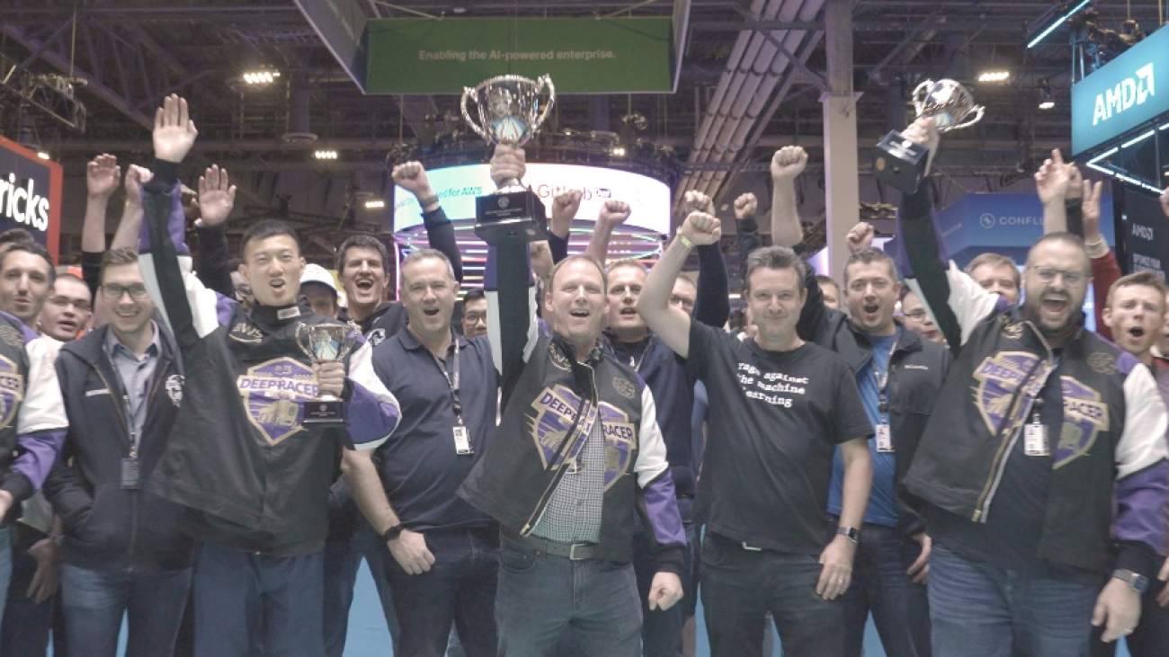
AWS DeepRacer League 2024 Championship finalists at re:Invent 2024
The AWS DeepRacer League is the world’s first global autonomous racing league powered by machine learning (ML). Over the past 6 years, a diverse community of over 560,000 builders from more than 150 countries worldwide have participated in the League to learn ML fundamentals hands-on through the fun of friendly autonomous racing. After an 8-month season of nail-biting virtual qualifiers, finalists convened in person at re:Invent in Las Vegas for one final showdown to compete for prizes and glory in the high-stakes, winner-take-all AWS DeepRacer League Championship. It wasn’t just the largest prize purse in DeepRacer history or the bragging rights of being the fastest builder in the world that was on the line—2024 marked the final year of the beloved League, and the winner of the 2024 Championship would also have the honor of being the very last AWS DeepRacer League Champion.
Tens of thousands raced in Virtual Circuit monthly qualifiers from March to October in an attempt to earn one of only four spots from six regions (24 spots in all), making qualifying for the 2024 Championship one of the most difficult to date. Finalists were tested on consistent performance over consecutive laps rather than “one lucky lap,” making the championship a true test of skill and dashing the championship dreams of some of the most prolific racers, community leaders, and former championship finalists during the regular season. When the dust settled, the best of the best from around the world secured their spots in the championship alongside returning 2023 champion FiatLux (Youssef Addioui) and 2023 Open Winner PolishThunder (Daryl Jezierski). For the rest of the hopefuls, there was only one more opportunity—the WildCard Last Chance qualifier on the Expo floor at re:Invent 2024—to gain entry into the final championship and etch their names in the annals of DeepRacer history.
In a tribute to the League’s origins, the Forever Raceway was chosen as the final championship track. This adaptation of the RL Speedway, which made its initial debut at the DeepRacer League Summit Circuit in 2022, presented a unique challenge: it’s nearly 30% narrower than tracks from the last five seasons, returning to a width only seen in the inaugural League season. The 76-centimeter-wide track leaves little room for error because it exaggerates the curves of the course and forces the vehicle to follow the track contours closely to stay within the borders.
The Wildcard Last Chance
As the Wildcard began on Monday night, the sidelines were packed with a mix of DeepRacer royalty and fresh-faced contenders, all vying for one of the coveted six golden tickets to round 1 of the championship. Twenty elite racers from all corners of the globe unleashed their best models onto the track, each looking for three clean laps (no off-tracks) in a mere 120 seconds to take their place alongside the Virtual Circuit champions.
The following image displays the 2024 qualifiers.

Newcomer and JP Morgan Chase (JPMC) DeepRacer Women’s League winner geervani (Geervani Kolukuluri) made her championship debut, dominating the competition early and showing the crowd exactly why she was the best of the league’s 829 participants and one of the top racers of the 4,400 that participated from JP Morgan Chase in 2024. She was nipping at the heels of community leader, DeepRacer for Cloud contributor, and Wildcard pack leader MattCamp, and less than a second behind SimonHill, another championship rookie and winner of the Eviden internal league.
But the old guard wasn’t about to go down without a fight. DeepRacer legend LeadingAI (Jacky Chen), an educator and mentor to Virtual Circuit winner AIDeepRacer (Nathan Liang), landed the fourth best time of 9.527, slightly ahead of Jerec (Daniel Morgan), who returned to the finals after taking third place in the 2023 Championship. Duckworth (Lars Ludvigson), AWS Community Builder and solutions developer, took the sixth and final Wildcard spot, less than three-tenths of a second above the rest of the pack.

The field of 32 begins
The first 16 of 32 code warriors hit the track on Tuesday, each one going for glory in two heart-pounding, 2-minute sprints to secure their spot in the bracket of eight over 2 days of competition. MattCamp proved he was no one-hit wonder by blazing across the finish line with Tuesday’s fastest time of 8.223 seconds, geervani still just milliseconds behind at 8.985. Asian Pacific regional stars TonyJ (Tony Jenness) and CodeMachine (Igor Maksaev Brockway) came out swinging, claiming their place in the top four just ahead of 2023 champion FiatLux of the EMEA region, who dug deep to stay in the game, finishing fifth with a time of 9.223. Liao (Wei-Chen Liao), Nevertari (Neveen Ahmed), and BSi (Bobby Stenly) also edged above the pack as the day of racing ended, their positions precarious as they hovered just inside the top eight for the day.
The tension was high and the stands full on Wednesday as the second day of Round 1 racing began, the second 16 ready to burn rubber and leave the Tuesday competitors in the dust. AIDeepRacer (Nathan Liang) quickly dethroned MattCamp with a blistering time of 8.102, looking to redeem himself from barely missing the bracket of eight in the 2022 Championship. 2023 Global points winner rosscomp1 (Ross Williams) slid into the top four right behind the indomitable SimonHill, while geervani, TonyJ, and CodeMachine managed to stay in the game as the Wednesday racers tried to best their times.
A mechanical failure in his second attempt gave community leader MarkRoss one last attempt to break into the top eight. His 8.635-second run looked like it might just be his ticket to Round 2, but a challenge from the sidelines had everyone holding their breath. The tension was palpable as the DeepRacer Pit Crew reviewed video footage to determine if Mark’s car had stayed within track limits, knowing that a spot in the semifinals—and a shot at the $25,000 grand prize—hung in the balance. Mark’s hopes were dashed when the replay revealed all four wheels left the track, and PolishThunder snuck into Round 2 by the skin of their teeth, claiming the coveted eighth-place spot.
The following images show Blaine Sundrud and Ryan Myrehn commentating on Round 2 (left) and the off-track footage (right).

And then there were eight
On Thursday morning, racers and spectators returned to the Forever Raceway for the bracket of eight, a series of head-to-head battles pitting the top racers against each other in a grueling double elimination format. Each matchup was another contest of speed and accuracy, another chance for the undefeatable to be toppled from their thrones and underdogs to scrap their way back into contention in the last chance bracket, as shown in the following image.

First seed AIDeepRacer dominated their first two matchups, sending rosscomp1 and PolishThunder to early defeat, definitively earning a place in the final three. Sixth seed TonyJ couldn’t get his average lap under 12 seconds against third seed SimonHill, while fellow regional heavyweight CodeMachine was unable to close the 1-second gap between him and second seed MattCamp, the strong favorite coming out of the Wildcard and round 1. That left MattCamp and SimonHill to one last battle for a place in the top three, with SimonHill finally gaining the upper hand in a 9.026- to 9.478-second shootout, sending MattCamp to the Last Chance bracket to try to fight his way back to the top.
With one final spot in the top three up for grabs, five-time championship finalist and eighth-seed PolishThunder, who was stunned into defeat in the very first matchup of the day, mounted an equally stunning comeback as he bested fifth seed geervani in match five and then knocked out fellow DeepRacer veteran, friend, and fourth-seed rosscomp1 with a remarkable 8.389-second time. MattCamp regained his mojo to beat TonyJ in match 10, setting him and PolishThunder up for a showdown to see who would go up against SimonHill and AIDeepRacer in the finale. Undaunted, PolishThunder toppled the Wildcard winner once and for all, taking him one step closer to being the DeepRacer Champion.
The final three
After almost 4 days of triumph and heartbreak, only three competitors remained for one final winner-take-all time trial that would determine, for the last time, the fastest builder in the world. Commentators Ryan Myrehn and Blaine Sundrud, who have been with the DeepRacer program since the very beginning, took to the mic together as the sidelines filled with finalists, spectators, and Pit Crew eager to see who would take home the championship trophy.
Prior to their final lap, each racer was able to choose a car and calibrate it to their liking, giving them an opportunity to optimize for the best performance with their chosen model. A coin toss decided the racing direction, counterclockwise, and each was given 1 minute to test the newly calibrated cars to make sure they were happy with their adjustments. With three cars tested, calibrated, and loaded with their best models, it was down to just 6 minutes of racing that would determine the 2024 Champion.
PolishThunder took to the track first, starting the finale strong as his model averaged a mere 8.436 seconds in laps five, six, and seven, setting a high bar for his competitors. SimonHill answered with a blazing 8.353 seconds, the fastest counterclockwise average of the competition, edging out the comeback king with less than a pixel’s width between them. Then, with just one race left, the crowd watched with bated breath as the competition’s top seed AIDeepRacer approached the starting line, hoping to replicate his enviable lap times from previous rounds. After a tense 2 minutes, first-time competitor SimonHill held onto first place, winning the $25,000 grand prize, the coveted DeepRacer trophy, and legendary status as the final DeepRacer champion. PolishThunder, who previously hadn’t broken the top six in his DeepRacer career, finished second, and AIDeepRacer third for his second, and best, championship appearance since his debut in 2022.
As the final chapter came to a close and trophies were handed out, racers and Pit Crew who have worked, competed, and built lifelong friendships around a 1/18th scale autonomous car celebrated together one more time on the very last championship track. Although the League may have concluded, the legacy of DeepRacer and its unique ability to teach ML and the foundations of generative AI through gamified learning continues. Support for DeepRacer in the AWS console will continue through the end of 2025, and DeepRacer will enter a new era as organizations around the world will also be able to launch their own leagues and competitions at a fraction of the cost with the AWS DeepRacer Solution. Featuring the same functionality as the console and deployable anywhere, the Solution will also contain new workshops and resources bridging fundamental concepts of ML using AWS DeepRacer with foundation model (FM) training and fine-tuning techniques, using AWS services such as Amazon SageMaker and Amazon Bedrock for popular industry use cases. Look for the Solution to kickstart your company’s ML transformation starting in Q2 of 2025.
The following images show championship finalists and pit crew at re:Invent 2024 (left) and 2024 League Champion Simon Hill with his first-place trophy (right).
 |
 |
Join the DeepRacer community at deepracing.io.
About the Author
 Jackie Moffett is a Senior Project Manager in the AWS AI Builder Programs Product Marketing team. She believes hands-on is the best way to learn and is passionate about building better systems to create exceptional customer experiences. Outside of work she loves to travel, is addicted to learning new things, and definitely wants to say hi to your dog.

Evaluate healthcare generative AI applications using LLM-as-a-judge on AWS
In our previous blog posts, we explored various techniques such as fine-tuning large language models (LLMs), prompt engineering, and Retrieval Augmented Generation (RAG) using Amazon Bedrock to generate impressions from the findings section in radiology reports using generative AI. Part 1 focused on model fine-tuning. Part 2 introduced RAG, which combines LLMs with external knowledge bases to reduce hallucinations and improve accuracy in medical applications. Through real-time retrieval of relevant medical information, RAG systems can provide more reliable and contextually appropriate responses, making them particularly valuable for healthcare applications where precision is crucial. In both previous posts, we used traditional metrics like ROUGE scores for performance evaluation. This metric is suitable for evaluating general summarization tasks, but can’t effectively assess whether a RAG system successfully integrates retrieved medical knowledge or maintains clinical accuracy.
In Part 3, we’re introducing an approach to evaluate healthcare RAG applications using LLM-as-a-judge with Amazon Bedrock. This innovative evaluation framework addresses the unique challenges of medical RAG systems, where both the accuracy of retrieved medical knowledge and the quality of generated medical content must align with stringent standards such as clear and concise communication, clinical accuracy, and grammatical accuracy. By using the latest models from Amazon and the newly released RAG evaluation feature for Amazon Bedrock Knowledge Bases, we can now comprehensively assess how well these systems retrieve and use medical information to generate accurate, contextually appropriate responses.
This advancement in evaluation methodology is particularly crucial as healthcare RAG applications become more prevalent in clinical settings. The LLM-as-a-judge approach provides a more nuanced evaluation framework that considers both the quality of information retrieval and the clinical accuracy of generated content, aligning with the rigorous standards required in healthcare.
In this post, we demonstrate how to implement this evaluation framework using Amazon Bedrock, compare the performance of different generator models, including Anthropic’s Claude and Amazon Nova on Amazon Bedrock, and showcase how to use the new RAG evaluation feature to optimize knowledge base parameters and assess retrieval quality. This approach not only establishes new benchmarks for medical RAG evaluation, but also provides practitioners with practical tools to build more reliable and accurate healthcare AI applications that can be trusted in clinical settings.
Overview of the solution
The solution uses Amazon Bedrock Knowledge Bases evaluation capabilities to assess and optimize RAG applications specifically for radiology findings and impressions. Let’s examine the key components of this architecture in the following figure, following the data flow from left to right.

The workflow consists of the following phases:
- Data preparation – Our evaluation process begins with a prompt dataset containing paired radiology findings and impressions. This clinical data undergoes a transformation process where it’s converted into a structured JSONL format, which is essential for compatibility with the knowledge base evaluation system. After it’s prepared, this formatted data is securely uploaded to an Amazon Simple Storage Service (Amazon S3) bucket, providing accessibility and data security throughout the evaluation process.
- Evaluation processing – At the heart of our solution lies an Amazon Bedrock Knowledge Bases evaluation job. This component processes the prepared data while seamlessly integrating with Amazon Bedrock Knowledge Bases. This integration is crucial because it enables the system to create specialized medical RAG capabilities specifically tailored for radiology findings and impressions, making sure that the evaluation considers both medical context and accuracy.
- Analysis – The final stage empowers healthcare data scientists with detailed analytical capabilities. Through an advanced automated report generation system, professionals can access detailed analysis of performance metrics of the summarization task for impression generation. This comprehensive reporting system enables thorough assessment of both retrieval quality and generation accuracy, providing valuable insights for system optimization and quality assurance.
This architecture provides a systematic and thorough approach to evaluating medical RAG applications, providing both accuracy and reliability in healthcare contexts where precision and dependability are paramount.
Dataset and background
The MIMIC Chest X-ray (MIMIC-CXR) database v2.0.0 is a large, publicly available dataset of chest radiographs in DICOM format with free-text radiology reports. We used the MIMIC CXR dataset consisting of 91,544 reports, which can be accessed through a data use agreement. This requires user registration and the completion of a credentialing process.
During routine clinical care, clinicians trained in interpreting imaging studies (radiologists) will summarize their findings for a particular study in a free-text note. The reports were de-identified using a rule-based approach to remove protected health information. Because we used only the radiology report text data, we downloaded just one compressed report file (mimic-cxr-reports.zip) from the MIMIC-CXR website. For evaluation, 1,000 of the total 2,000 reports from a subset of MIMIC-CXR dataset were used. This is referred to as the dev1 dataset. Another set of 1,000 of the total 2,000 radiology reports (referred to as dev2) from the chest X-ray collection from the Indiana University hospital network were also used.
RAG with Amazon Bedrock Knowledge Bases
Amazon Bedrock Knowledge Bases helps take advantage of RAG, a popular technique that involves drawing information from a data store to augment the responses generated by LLMs. We used Amazon Bedrock Knowledge Bases to generate impressions from the findings section of the radiology reports by enriching the query with context that is received from querying the knowledge base. The knowledge base is set up to contain findings and corresponding impression sections of 91,544 MIMIC-CXR radiology reports as {prompt, completion} pairs.
LLM-as-a-judge and quality metrics
LLM-as-a-judge represents an innovative approach to evaluating AI-generated medical content by using LLMs as automated evaluators. This method is particularly valuable in healthcare applications where traditional metrics might fail to capture the nuanced requirements of medical accuracy and clinical relevance. By using specialized prompts and evaluation criteria, LLM-as-a-judge can assess multiple dimensions of generated medical content, providing a more comprehensive evaluation framework that aligns with healthcare professionals’ standards.
Our evaluation framework encompasses five critical metrics, each designed to assess specific aspects of the generated medical content:
- Correctness – Evaluated on a 3-point Likert scale, this metric measures the factual accuracy of generated responses by comparing them against ground truth responses. In the medical context, this makes sure that the clinical interpretations and findings align with the source material and accepted medical knowledge.
- Completeness – Using a 5-point Likert scale, this metric assesses whether the generated response comprehensively addresses the prompt holistically while considering the ground truth response. It makes sure that critical medical findings or interpretations are not omitted from the response.
- Helpfulness – Measured on a 7-point Likert scale, this metric evaluates the practical utility of the response in clinical contexts, considering factors such as clarity, relevance, and actionability of the medical information provided.
- Logical coherence – Assessed on a 5-point Likert scale, this metric examines the response for logical gaps, inconsistencies, or contradictions, making sure that medical reasoning flows naturally and maintains clinical validity throughout the response.
- Faithfulness – Scored on a 5-point Likert scale, this metric specifically evaluates whether the response contains information not found in or quickly inferred from the prompt, helping identify potential hallucinations or fabricated medical information that could be dangerous in clinical settings.
These metrics are normalized in the final output and job report card, providing standardized scores that enable consistent comparison across different models and evaluation scenarios. This comprehensive evaluation framework not only helps maintain the reliability and accuracy of medical RAG systems, but also provides detailed insights for continuous improvement and optimization. For details about the metric and evaluation prompts, see Evaluator prompts used in a knowledge base evaluation job.
Prerequisites
Before proceeding with the evaluation setup, make sure you have the following:
- An active AWS account with appropriate permissions
- Amazon Bedrock model access enabled in your preferred AWS Region
- An S3 bucket with CORS enabled for storing evaluation data
- An Amazon Bedrock knowledge base
- An AWS Identity and Access Management (IAM) role with necessary permissions for Amazon S3 and Amazon Bedrock
The solution code can be found at the following GitHub repo.
Make sure that your knowledge base is fully synced and ready before initiating an evaluation job.
Convert the test dataset into JSONL for RAG evaluation
In preparation for evaluating our RAG system’s performance on radiology reports, we implemented a data transformation pipeline to convert our test dataset into the required JSONL format. The following code shows the format of the original dev1 and dev2 datasets:
{
    "prompt": "value of prompt key",
    "completion": "value of completion key"
}
Output Format

{
    "conversationTurns": [{
        "referenceResponses": [{
            "content": [{
                "text": "value from completion key"
            }]
        }],
        "prompt": {
            "content": [{
                "text": "value from prompt key"
            }]
        }
    }]
}
Drawing from Wilcox’s seminal paper The Written Radiology Report, we carefully structured our prompt to include comprehensive guidelines for generating high-quality impressions:
import json
import random
import boto3

# Initialize the S3 client
s3 = boto3.client('s3')

# S3 bucket name
bucket_name = "<BUCKET_NAME>"

# Function to transform a single record
def transform_record(record):
    return {
        "conversationTurns": [
            {
                "referenceResponses": [
                    {
                        "content": [
                            {
                                "text": record["completion"]
                            }
                        ]
                    }
                ],
                "prompt": {
                    "content": [
                        {
                            "text": """You're given a radiology report findings to generate a concise radiology impression from it.

A Radiology Impression is the radiologist's final concise interpretation and conclusion of medical imaging findings, typically appearing at the end of a radiology report.
n Follow these guidelines when writing the impression:
n- Use clear, understandable language avoiding obscure terms.
n- Number each impression.
n- Order impressions by importance.
n- Keep impressions concise and shorter than the findings section.
n- Write for the intended reader's understanding.n
Findings: n""" + record["prompt"]
                        }
                    ]
                }
            }
        ]
    }
The script processes individual records, restructuring them to include conversation turns with both the original radiology findings and their corresponding impressions, making sure each report maintains the professional standards outlined in the literature. To maintain a manageable dataset size set used by this feature, we randomly sampled 1,000 records from the original dev1 and dev2 datasets, using a fixed random seed for reproducibility:
# Read from input file and write to output file
def convert_file(input_file_path, output_file_path, sample_size=1000):
    # First, read all records into a list
    records = []
    with open(input_file_path, 'r', encoding='utf-8') as input_file:
        for line in input_file:
            records.append(json.loads(line.strip()))

    # Randomly sample 1000 records
    random.seed(42)  # Set the seed first
    sampled_records = random.sample(records, sample_size)

    # Write the sampled and transformed records to the output file
    with open(output_file_path, 'w', encoding='utf-8') as output_file:
        for record in sampled_records:
            transformed_record = transform_record(record)
            output_file.write(json.dumps(transformed_record) + 'n')

# Usage
input_file_path = '<INPUT_FILE_NAME>.jsonl'  # Replace with your input file path
output_file_path = '<OUTPUT_FILE_NAME>.jsonl'  # Replace with your desired output file path
convert_file(input_file_path, output_file_path)

# File paths and S3 keys for the transformed files
transformed_files = [
    {'local_file': '<OUTPUT_FILE_NAME>.jsonl', 'key': '<FOLDER_NAME>/<OUTPUT_FILE_NAME>.jsonl'},
    {'local_file': '<OUTPUT_FILE_NAME>.jsonl', 'key': '<FOLDER_NAME>/<OUTPUT_FILE_NAME>.jsonl'}
]

# Upload files to S3
for file in transformed_files:
    s3.upload_file(file['local_file'], bucket_name, file['key'])
    print(f"Uploaded {file['local_file']} to s3://{bucket_name}/{file['key']}")
Set up a RAG evaluation job
Our RAG evaluation setup begins with establishing core configurations for the Amazon Bedrock evaluation job, including the selection of evaluation and generation models (Anthropic’s Claude 3 Haiku and Amazon Nova Micro, respectively). The implementation incorporates a hybrid search strategy with a retrieval depth of 10 results, providing comprehensive coverage of the knowledge base during evaluation. To maintain organization and traceability, each evaluation job is assigned a unique identifier with timestamp information, and input data and results are systematically managed through designated S3 paths. See the following code:
import boto3
from datetime import datetime

# Generate unique name for the job
job_name = f"rag-eval-{datetime.now().strftime('%Y-%m-%d-%H-%M-%S')}"

# Configure knowledge base and model settings
knowledge_base_id = "<KNOWLEDGE_BASE_ID>"
evaluator_model = "anthropic.claude-3-haiku-20240307-v1:0"
generator_model = "amazon.nova-micro-v1:0"
role_arn = "<IAM_ROLE_ARN>"

# Specify S3 locations
input_data = "<INPUT_S3_PATH>"
output_path = "<OUTPUT_S3_PATH>"

# Configure retrieval settings
num_results = 10
search_type = "HYBRID"

# Create Bedrock client
bedrock_client = boto3.client('bedrock')
With the core configurations in place, we initiate the evaluation job using the Amazon Bedrock create_evaluation_job API, which orchestrates a comprehensive assessment of our RAG system’s performance. The evaluation configuration specifies five key metrics—correctness, completeness, helpfulness, logical coherence, and faithfulness—providing a multi-dimensional analysis of the generated radiology impressions. The job is structured to use the knowledge base for retrieval and generation tasks, with the specified models handling their respective roles: Amazon Nova Micro for generation and Anthropic’s Claude 3 Haiku for evaluation, and the results are systematically stored in the designated S3 output location for subsequent analysis. See the following code:
retrieve_generate_job = bedrock_client.create_evaluation_job(
    jobName=job_name,
    jobDescription="Evaluate retrieval and generation",
    roleArn=role_arn,
    applicationType="RagEvaluation",
    inferenceConfig={
        "ragConfigs": [{
            "knowledgeBaseConfig": {
                "retrieveAndGenerateConfig": {
                    "type": "KNOWLEDGE_BASE",
                    "knowledgeBaseConfiguration": {
                        "knowledgeBaseId": knowledge_base_id,
                        "modelArn": generator_model,
                        "retrievalConfiguration": {
                            "vectorSearchConfiguration": {
                                "numberOfResults": num_results,
                                "overrideSearchType": search_type
                            }
                        }
                    }
                }
            }
        }]
    },
    outputDataConfig={
        "s3Uri": output_path
    },
    evaluationConfig={
        "automated": {
            "datasetMetricConfigs": [{
                "taskType": "Custom",
                "dataset": {
                    "name": "RagDataset",
                    "datasetLocation": {
                        "s3Uri": input_data
                    }
                },
                "metricNames": [
                    "Builtin.Correctness",
                    "Builtin.Completeness",
                    "Builtin.Helpfulness",
                    "Builtin.LogicalCoherence",
                    "Builtin.Faithfulness"
                ]
            }],
            "evaluatorModelConfig": {
                "bedrockEvaluatorModels": [{
                    "modelIdentifier": evaluator_model
                }]
            }
        }
    }
)
Evaluation results and metrics comparisons
The evaluation results for the healthcare RAG applications, using datasets dev1 and dev2, demonstrate strong performance across the specified metrics. For the dev1 dataset, the scores were as follows: correctness at 0.98, completeness at 0.95, helpfulness at 0.83, logical coherence at 0.99, and faithfulness at 0.79. Similarly, the dev2 dataset yielded scores of 0.97 for correctness, 0.95 for completeness, 0.83 for helpfulness, 0.98 for logical coherence, and 0.82 for faithfulness. These results indicate that the RAG system effectively retrieves and uses medical information to generate accurate and contextually appropriate responses, with particularly high scores in correctness and logical coherence, suggesting robust factual accuracy and logical consistency in the generated content.
The following screenshot shows the evaluation summary for the dev1 dataset.

The following screenshot shows the evaluation summary for the dev2 dataset.

Additionally, as shown in the following screenshot, the LLM-as-a-judge framework allows for the comparison of multiple evaluation jobs across different models, datasets, and prompts, enabling detailed analysis and optimization of the RAG system’s performance.

Additionally, you can perform a detailed analysis by drilling down and investigating the outlier cases with least performance metrics such as correctness, as shown in the following screenshot.

Metrics explainability
The following screenshot showcases the detailed metrics explainability interface of the evaluation system, displaying example conversations with their corresponding metrics assessment. Each conversation entry includes four key columns: Conversation input, Generation output, Retrieved sources, and Ground truth, along with a Score column. The system provides a comprehensive view of 1,000 examples, with navigation controls to browse through the dataset. Of particular note is the retrieval depth indicator showing 10 for each conversation, demonstrating consistent knowledge base utilization across examples.
The evaluation framework enables detailed tracking of generation metrics and provides transparency into how the knowledge base arrives at its outputs. Each example conversation presents the complete chain of information, from the initial prompt through to the final assessment. The system displays the retrieved context that informed the generation, the actual generated response, and the ground truth for comparison. A scoring mechanism evaluates each response, with a detailed explanation of the decision-making process visible through an expandable interface (as shown by the pop-up in the screenshot). This granular level of detail allows for thorough analysis of the RAG system’s performance and helps identify areas for optimization in both retrieval and generation processes.

In this specific example from the Indiana University Medical System dataset (dev2), we see a clear assessment of the system’s performance in generating a radiology impression for chest X-ray findings. The knowledge base successfully retrieved relevant context (shown by 10 retrieved sources) to generate an impression stating “Normal heart size and pulmonary vascularity 2. Unremarkable mediastinal contour 3. No focal consolidation, pleural effusion, or pneumothorax 4. No acute bony findings.” The evaluation system scored this response with a perfect correctness score of 1, noting in the detailed explanation that the candidate response accurately summarized the key findings and correctly concluded there was no acute cardiopulmonary process, aligning precisely with the ground truth response.

In the following screenshot, the evaluation system scored this response with a low score of 0.5, noting in the detailed explanation the ground truth response provided is “Moderate hiatal hernia. No definite pneumonia.” This indicates that the key findings from the radiology report are the presence of a moderate hiatal hernia and the absence of any definite pneumonia. The candidate response covers the key finding of the moderate hiatal hernia, which is correctly identified as one of the impressions. However, the candidate response also includes additional impressions that are not mentioned in the ground truth, such as normal lung fields, normal heart size, unfolded aorta, and degenerative changes in the spine. Although these additional impressions might be accurate based on the provided findings, they are not explicitly stated in the ground truth response. Therefore, the candidate response is partially correct and partially incorrect based on the ground truth.
Clean up
To avoid incurring future charges, delete the S3 bucket, knowledge base, and other resources that were deployed as part of the post.
Conclusion
The implementation of LLM-as-a-judge for evaluating healthcare RAG applications represents a significant advancement in maintaining the reliability and accuracy of AI-generated medical content. Through this comprehensive evaluation framework using Amazon Bedrock Knowledge Bases, we’ve demonstrated how automated assessment can provide detailed insights into the performance of medical RAG systems across multiple critical dimensions. The high-performance scores across both datasets indicate the robustness of this approach, though these metrics are just the beginning.
Looking ahead, this evaluation framework can be expanded to encompass broader healthcare applications while maintaining the rigorous standards essential for medical applications. The dynamic nature of medical knowledge and clinical practices necessitates an ongoing commitment to evaluation, making continuous assessment a cornerstone of successful implementation.
Through this series, we’ve demonstrated how you can use Amazon Bedrock to create and evaluate healthcare generative AI applications with the precision and reliability required in clinical settings. As organizations continue to refine these tools and methodologies, prioritizing accuracy, safety, and clinical utility in healthcare AI applications remains paramount.
About the Authors
 Adewale Akinfaderin is a Sr. Data Scientist–Generative AI, Amazon Bedrock, where he contributes to cutting edge innovations in foundational models and generative AI applications at AWS. His expertise is in reproducible and end-to-end AI/ML methods, practical implementations, and helping global customers formulate and develop scalable solutions to interdisciplinary problems. He has two graduate degrees in physics and a doctorate in engineering.
 Priya Padate is a Senior Partner Solution Architect supporting healthcare and life sciences worldwide at Amazon Web Services. She has over 20 years of healthcare industry experience leading architectural solutions in areas of medical imaging, healthcare related AI/ML solutions and strategies for cloud migrations. She is passionate about using technology to transform the healthcare industry to drive better patient care outcomes.
 Dr. Ekta Walia Bhullar is a principal AI/ML/GenAI consultant with AWS Healthcare and Life Sciences business unit. She has extensive experience in development of AI/ML applications for healthcare especially in Radiology. During her tenure at AWS she has actively contributed to applications of AI/ML/GenAI within lifescience domain such as for clinical, drug development and commercial lines of business.
AWS DeepRacer: Closing time at AWS re:Invent 2024 –How did that physical racing go?
Having spent the last years studying the art of AWS DeepRacer in the physical world, the author went to AWS re:Invent 2024. How did it go?
In AWS DeepRacer: How to master physical racing?, I wrote in detail about some aspects relevant to racing AWS DeepRacer in the physical world. We looked at the differences between the virtual and the physical world and how we could adapt the simulator and the training approach to overcome the differences. The previous post was left open-ended—with one last Championship Final left, it was too early to share all my secrets.
Now that AWS re:Invent is over, it’s time to share my strategy, how I prepared, and how it went in the end.
Strategy
Going into the 2024 season, I was reflecting on my performance from 2022 and 2023. In 2022, I had unstable models that were unable to do fast laps on the new re:Invent 2022 Championship track, not even making the last 32. In 2023, things went slightly better, but it was clear that there was potential to improve.
Specifically, I wanted a model that:
- Goes straight on the straights and corners with precision
- Has a survival instinct and avoids going off-track even in a tight spot
- Can ignore the visual noise seen around the track
Combine that with the ability to test the models before showing up at the Expo, and success seemed possible!
Implementation
In this section, I will explain my thinking about why physical racing is so different than virtual racing, as well as describe my approach to training a model that overcomes those differences.
How hard can it be to go straight?
If you have watched DeepRacer over the years, you have probably seen that most models struggle to go straight on the straights and end up oscillating left and right. The question has always been: why is it like that? This behavior causes two issues: the distance driven increases (result: slower lap time) and the car potentially enters the next turn in a way it can’t handle (result: off-track).
A few theories emerged:
- Sim-to-real issues – The steering response isn’t matching the simulator, both with regards to the steering geometry and latency (time from picture to servo command, as well as the time it takes the servo to actually actuate). Therefore, when the car tries to adjust the direction on the straight, it doesn’t get the response it expects.
- Model issues – A combination of the model not actually using the straight action, and not having access to angles needed to dampen oscillations (2.5–5.0 degrees).
- Calibration issues – If the car isn’t calibrated to go straight when given a 0-degree action, and the left/right max values are either too high (tendency to oversteer) or too low (tendency to understeer), you are likely to get control issues and unstable behavior.
My approach:
- Use the Ackermann steering geometry patch. With it, the car will behave more realistically, and the turning radius will decrease for a given angle. As a result, the action space can be limited to angles up to about 20 degrees. This roughly matches with the real car’s steering angle.
- Include stabilizing steering angles (2.5 and 5.0) in the action space, allowing for minor corrections on the straights.
- Use relatively slow speeds (0.8–1.3 m/s) to avoid slipping in the simulator. My theory is that the 15 fps simulator and the 30 fps car actually translates 1.2 mps in the simulator into effectively 2.4 mps in the real world.
- By having an inverted chevron action space giving higher speeds for straights, nudge the car to use the straight actions, rather than oscillating left-right actions.
- Try out v3, v4, and v5 physical models—test on a real track to see what works best.
- Otherwise, the reward function was the same progress-based reward function I also use in virtual racing.
The following figure illustrates the view of testing in the garage, going straight at least one frame.

Be flexible
Virtual racing is (almost) deterministic, and over time, the model will converge and the car will take a narrow path, reducing the variety in the situations it sees. Early in training, it will frequently be in odd positions, almost going off-track, and it remembers how to get out of these situations. As it converges, the frequency at which it must handle these reduces, and the theory is that the memory fades, and at some point, it forgets how to get out of a tight spot.
My approach:
- Diversify training to teach the car to handle a variety of corners, in both directions:
- Consistently train models going both clockwise and counterclockwise.
- Use tracks—primarily the 2022 Championship track—that are significantly more complex than the Forever Raceway.
- Do final optimization on the Forever Raceway—again in both directions.
- Take several snapshots during training; don’t go below 0.5 in entropy.
- Test on tracks the car has never seen. The simulator has many suitable, narrow tracks—the hallmark of a generalized model is one that can handle tracks it has never seen during training.
Stay focused on the track
In my last post, I looked at the visual differences between the virtual and real worlds. The question is what to do about it. The goal is to trick the model into ignoring the noise and focus on what is important: the track.
My approach:
- Train in an environment with significantly more visual noise. The tracks in the custom track repository have added noise through additional lights, buildings, and different walls (and some even come with shadows).
- Alter the environment during training to avoid overfitting to the added noise. The custom tracks were made in such a way that different objects (buildings, walls, and lines) could be made invisible at runtime. I had a cron job randomizing the environment every 5 minutes.
The following figure illustrates the varied training environment.

What I didn’t consider this year was simulating blurring during training. I attempted this previously by averaging the current camera frame with the previous one before inferencing. It didn’t seem to help.
Lens distortion is a topic I have observed, but not fully investigated. The original camera has a distinct fish-eye distortion, and Gazebo would be able to replicate it, but it would require some work to actually determine the coefficients. Equally, I have never tried to replicate the rolling motions of the real car.
Testing
Testing took place in the garage on the Trapezoid Narrow track. The track is obviously basic, but with two straights and two 180-degree turns with different radii, it had to do the job. The garage track also had enough visual noise to see if the models were robust enough.
The method was straightforward: try all models both clockwise and counterclockwise. Using the logs captured by the custom car stack, I spent the evening looking through the video of each run to determine which model I liked the best—looking at stability, handling (straight on straights plus precision cornering), and speed.
re:Invent 2024
The track for re:Invent 2024 was the Forever Raceway. The shape of the track isn’t new; it shares the centerline with the 2022 Summit Speedway, but being only 76 cm wide (the original was 1.07 cm), the turns become more pronounced, making it a significantly more difficult track.
The environment
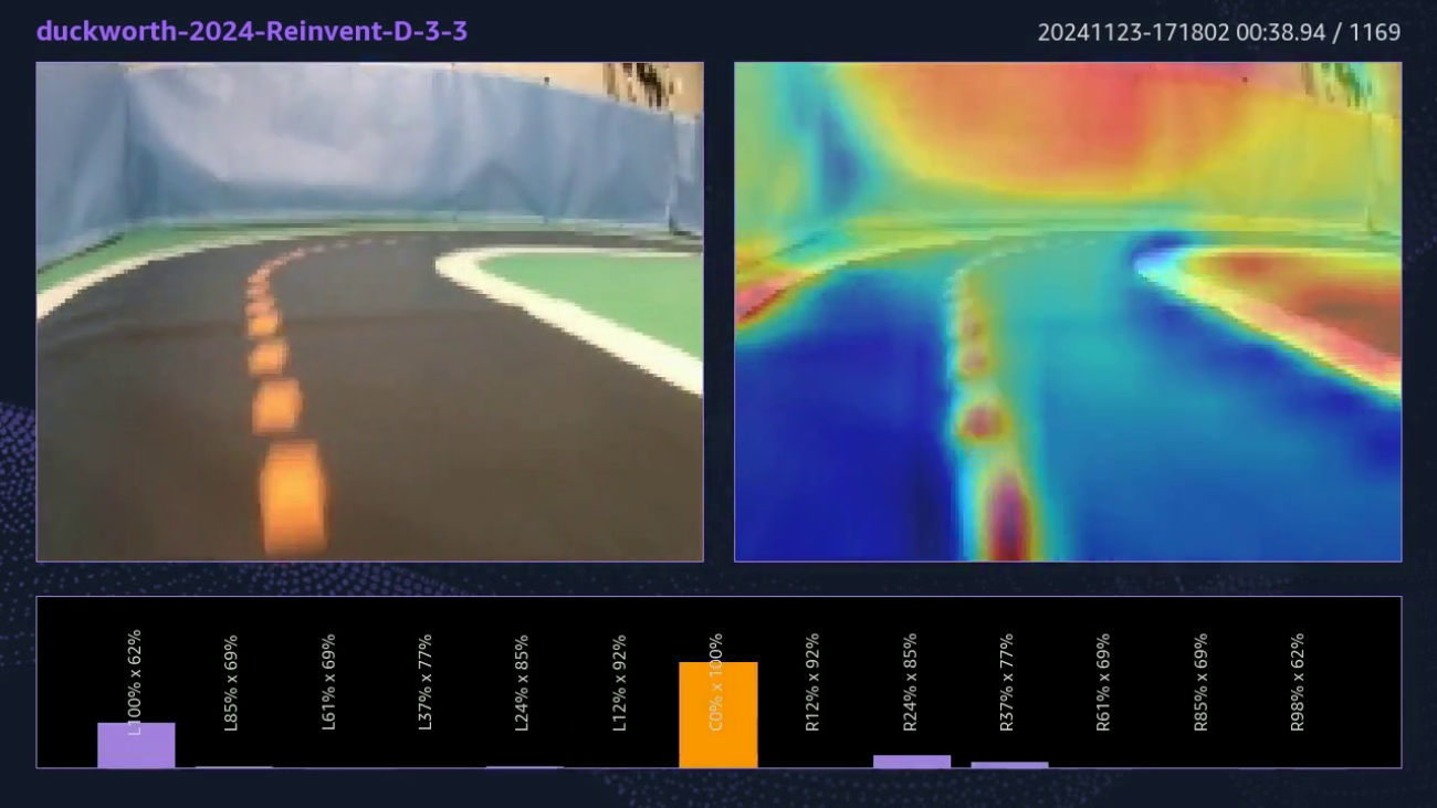
The environment is classic re:Invent: a smooth track with very little shine combined with smooth, fairly tall walls surrounding the track. The background is what often causes trouble—this year, a large lit display hung under the ceiling at the far end of the track, and as the following figure shows, it was attracting quite some attention from the GradCam.

Similarly, the pit crew cage, where cars are maintained, attracted attention.

The results
So where did I end up, and why? In Round 1, I ended up at place 14, with a best average of 10.072 seconds, and a best lap time of 9.335 seconds. Not great, but also not bad—almost 1 second outside top 8.
Using the overhead camera provided by AWS through the Twitch stream, it’s possible to create a graphical view showing the path the car took, as shown in the following figure.

If we compare this with how the same model liked to drive in training, we see a bit of a difference.

What becomes obvious quite quickly is that although I succeeded in going straight on the (upper) straight, the car didn’t corner as tightly as during training, making the bottom half of the track a bit of a mess. Nevertheless, the car demonstrated the desired survival instinct and stayed on track even when faced with unexpectedly sharp corners.
Why did this happen:
- 20 degrees of turning using Ackermann steering is too much; the real car isn’t capable of doing it in the real world
- The turning radius is increasing as the speed goes up due to slipping, caused both by low friction and lack of grip due to rolling
- The reaction time plays more of a role as the speed increases, and my model acted too late, overshooting into the corner
The combined turning radius and reaction time effect also caused issues at the start. If the car goes slowly, it turns much faster—and ends up going off-track on the inside—causing issues for me and others.

My takeaways:
- Overall, the training approach seemed to work well. Well-calibrated cars went straight on the straights, and background noise didn’t seem to bother my models much.
- I need to get closer to the car’s actual handling characteristics at speed during training by increasing the max speed and reducing the max angle in the action space.
- Physical racing is still not well understood—and it’s a lot about model-meets-car. Some models thrive on objectively perfectly calibrated cars, whereas others work great when matched with a particular one.
- Track is king—those that had access to the track, either through their employer or having built one at home, had a massive advantage, even if almost everyone said that they were surprised by which model worked in the end.
Now enjoy the inside view of a car at re:Invent, and see if you can detect any of the issues that I have discussed. The video was recorded after I had been knocked out of the competition using a car with the custom car software.
Closing time: Where do we go from here?
This section is best enjoyed with Semisonic’s Closing Time as a soundtrack.
As we all wrapped up at the Expo after an intense week of racing, re:Invent literally being dismantled around us, the question was: what comes next?
This was the last DeepRacer Championship, but the general sentiment was that whereas nobody will really miss virtual racing—it is a problem solved—physical racing is still a whole lot of fun, and the community is not yet ready to move on. Since re:Invent several initiatives have gained traction with a common goal to make DeepRacer more accessible:
- By enrolling cars with the DeepRacer Custom Car software stack into DeepRacer Event Manager you can capture car logs and generate the analytics videos, as shown in this article, directly during your event!
- DeepRacer Pi and DeepRacer Custom Car initiatives allow racers to build cars at home:Use off-the-shelf components for a 1:18 scale racer, or
- Combine off-the-shelf components with a custom circuit board to build the 1:28 scale DeepRacer Pi Mini Both options are compatible with already trained models, including integration with DeepRacer Event Manager.
DeepRacer Custom Console will be a drop-in replacement for the current car UI with a beautiful UI designed in Cloudscape, aligning the design with DREM and the AWS Console.

Prototype DeepRacer Pi Mini – 1 :28 scale
Closing Words
DeepRacer is a fantastic way to teach AI in a very physical and visual way, and is suitable for older kids, students, and adults in the corporate setting alike. It will be interesting to see how AWS, its corporate partners, and the community will continue the journey in the years ahead.
A big thank you goes to all of those that have been involved in DeepRacer from its inception to today—too many to be named—it has been a wonderful experience. A big congratulations goes out to this years’ winners!
Closing time, every new beginning comes from some other beginning’s end…

About the Author
Lars Lorentz Ludvigsen is a technology enthusiast who was introduced to AWS DeepRacer in late 2019 and was instantly hooked. Lars works as a Managing Director at Accenture, where he helps clients build the next generation of smart connected products. In addition to his role at Accenture, he’s an AWS Community Builder who focuses on developing and maintaining the AWS DeepRacer community’s software solutions.

Amazon announces Ocelot quantum chip
Amazon announces Ocelot quantum chip
Prototype is the first realization of a scalable, hardware-efficient quantum computing architecture based on bosonic quantum error correction.
Quantum technologies
Fernando Brando Oskar PainterFebruary 27, 06:00 AMApril 30, 08:32 PM
Today we are happy to announce Ocelot, our first-generation quantum chip. Ocelot represents Amazon Web Services pioneering effort to develop, from the ground up, a hardware implementation of quantum error correction that is both resource efficient and scalable. Based on superconducting quantum circuits, Ocelot achieves the following major technical advances:
- The first realization of a scalable architecture for bosonic error correction, surpassing traditional qubit approaches to reducing error correction overhead;
- The first implementation of a noise-biased gate a key to unlocking the type of hardware-efficient error correction necessary for building scalable, commercially viable quantum computers;
- State-of-the-art performance for superconducting qubits, with bit-flip times approaching one second in tandem with phase-flip times of 20 microseconds.

We believe that scaling Ocelot to a full-fledged quantum computer capable of transformative societal impact would require as little as one-tenth as many resources as common approaches, helping bring closer the age of practical quantum computing.
The quantum performance gap
Quantum computers promise to perform some computations much faster even exponentially faster than classical computers. This means quantum computers can solve some problems that are forever beyond the reach of classical computing.
Practical applications of quantum computing will require sophisticated quantum algorithms with billions of quantum gates the basic operations of a quantum computer. But current quantum computers extreme sensitivity to environmental noise means that the best quantum hardware today can run only about a thousand gates without error. How do we bridge this gap?
Quantum error correction: the key to reliable quantum computing
Quantum error correction, first proposed theoretically in the 1990s, offers a solution. By sharing the information in each logical qubit across multiple physical qubits, one can protect the information within a quantum computer from external noise. Not only this, but errors can be detected and corrected in a manner analogous to the classical error correction methods used in digital storage and communication.
Recent experiments have demonstrated promising progress, but todays best logical qubits, based on superconducting or atomic qubits, still exhibit error rates a billion times larger than the error rates needed for known quantum algorithms of practical utility and quantum advantage.
The challenge of qubit overhead
While quantum error correction provides a path to bridging the enormous chasm between todays error rates and those required for practical quantum computation, it comes with a severe penalty in terms of resource overhead. Reducing logical-qubit error rates requires scaling up the redundancy in the number of physical qubits per logical qubit.
Traditional quantum error correction methods, such as those using the surface error-correcting code, currently require thousands (and if we work really, really hard, maybe in the future, hundreds) of physical qubits per logical qubit to reach the desired error rates. That means that a commercially relevant quantum computer would require millions of physical qubits many orders of magnitude beyond the qubit count of current hardware.
One fundamental reason for this high overhead is that quantum systems experience two types of errors: bit-flip errors (also present in classical bits) and phase-flip errors (unique to qubits). Whereas classical bits require only correction of bit flips, qubits require an additional layer of redundancy to handle both types of errors.
Although subtle, this added complexity leads to quantum systems large resource overhead requirement. For comparison, a good classical error-correcting code could realize the error rate we desire for quantum computing with less than 30% overhead, roughly one-ten-thousandth the overhead of the conventional surface code approach (assuming bit error rates of 0.5%, similar to qubit error rates in current hardware).
Cat qubits: an approach to more efficient error correction
Quantum systems in nature can be more complex than qubits, which consist of just two quantum states (usually labeled 0 and 1 in analogy to classical digital bits). Take for example the simple harmonic oscillator, which oscillates with a well-defined frequency. Harmonic oscillators come in all sorts of shapes and sizes, from the mechanical metronome used to keep time while playing music to the microwave electromagnetic oscillators used in radar and communication systems.
Classically, the state of an oscillator can be represented by the amplitude and phase of its oscillations. Quantum mechanically, the situation is similar, although the amplitude and phase are never simultaneously perfectly defined, and there is an underlying graininess to the amplitude associated with each quanta of energy one adds to the system.
These quanta of energy are what are called bosonic particles, the best known of which is the photon, associated with the electromagnetic field. The more energy we pump into the system, the more bosons (photons) we create, and the more oscillator states (amplitudes) we can access. Bosonic quantum error correction, which relies on bosons instead of simple two-state qubit systems, uses these extra oscillator states to more effectively protect quantum information from environmental noise and to do more efficient error correction.
One type of bosonic quantum error correction uses cat qubits, named after the dead/alive Schrdinger cat of Erwin Schrdinger’s famous thought experiment. Cat qubits use the quantum superposition of classical-like states of well-defined amplitude and phase to encode a qubits worth of information. Just a few years after Peter Shors seminal 1995 paper on quantum error correction, researchers began quietly developing an alternative approach to error correction based on cat qubits.
A major advantage of cat qubits is their inherent protection against bit-flip errors. Increasing the number of photons in the oscillator can make the rate of the bit-flip errors exponentially small. This means that instead of increasing qubit count, we can simply increase the energy of an oscillator, making error correction far more efficient.
The past decade has seen pioneering experiments demonstrating the potential of cat qubits. However, these experiments have mostly focused on single-cat-qubit demonstrations, leaving open the question of whether cat qubits could be integrated into a scalable architecture.
Ocelot: demonstrating the scalability of bosonic quantum error correction
Today in Nature, we published the results of our measurements on Ocelot, and its quantum error correction performance. Ocelot represents an important step on the road to practical quantum computers, leveraging chip-scale integration of cat qubits to form a scalable, hardware-efficient architecture for quantum error correction. In this approach,
- bit-flip errors are exponentially suppressed at the physical-qubit level;
- phase-flip errors are corrected using a repetition code, the simplest classical error-correcting code; and
- highly noise-biased controlled-NOT (C-NOT) gates, between each cat qubit and ancillary transmon qubits (the conventional qubit used in superconducting quantum circuits), enable phase-flip-error detection while preserving the cats bit-flip protection.

The Ocelot logical-qubit memory chip, shown schematically above, consists of five cat data qubits, each housing an oscillator that is used to store the quantum data. The storage oscillator of each cat qubit is connected to two ancillary transmon qubits for phase-flip-error detection and paired with a special nonlinear buffer circuit used to stabilize the cat qubit states and exponentially suppress bit-flip errors.
Tuning up the Ocelot device involves calibrating the bit- and phase-flip error rates of the cat qubits against the cat amplitude (average photon number) and optimizing the noise-bias of the C-NOT gate used for phase-flip-error detection. Our experimental results show that we can achieve bit-flip times approaching one second, more than a thousand times longer than the lifetime of conventional superconducting qubits.
Critically, this can be accomplished with a cat amplitude as small as four photons, enabling us to retain phase-flip times of tens of microseconds, sufficient for quantum error correction. From there, we run a sequence of error correction cycles to test the performance of the circuit as a logical-qubit memory. In order to characterize the performance of the repetition code and the scalability of the architecture, we studied subsets of the Ocelot cat qubits, representing different repetition code lengths.
The logical phase-flip error rate was seen to drop significantly when the code distance was increased from distance-3 to distance-5 (i.e., from a code with three cat qubits to one with five) across a wide range of cat photon numbers, indicating the effectiveness of the repetition code.
When bit-flip errors were included, the total logical error rate was measured to be 1.72% per cycle for the distance-3 code and 1.65% per cycle for the distance-5 code. The comparability of the total error rate of the distance-5 code to that of the shorter distance-3 code, with fewer cat qubits and opportunities for bit-flip errors, can be attributed to the large noise bias of the C-NOT gate and its effectiveness in suppressing bit-flip errors. This noise bias is what allows Ocelot to achieve a distance-5 code with less than a fifth as many qubits five data qubits and four ancilla qubits, versus 49 qubits for a surface code device.
What we scale matters
From the billions of transistors in a modern GPU to the massive-scale GPU clusters powering AI models, the ability to scale efficiently is a key driver of technological progress. Similarly, scaling the number of qubits to accommodate the overhead required of quantum error correction will be key to realizing commercially valuable quantum computers.
But the history of computing shows that scaling the right component can have massive consequences for cost, performance, and even feasibility. The computer revolution truly took off when the transistor replaced the vacuum tube as the fundamental building block to scale.
Ocelot represents our first chip with the cat qubit architecture, and an initial test of its suitability as a fundamental building block for implementing quantum error correction. Future versions of Ocelot are being developed that will exponentially drive down logical error rates, enabled by both an improvement in component performance and an increase in code distance.
Codes tailored to biased noise, such as the repetition code used in Ocelot, can significantly reduce the number of physical qubits required. In our forthcoming paper Hybrid cat-transmon architecture for scalable, hardware-efficient quantum error correction, we find that scaling Ocelot could reduce quantum error correction overhead by up to 90% compared to conventional surface code approaches with similar physical-qubit error rates.
We believe that Ocelot’s architecture, with its hardware-efficient approach to error correction, positions us well to tackle the next phase of quantum computing: learning how to scale. Using a hardware-efficient approach will allow us to more quickly and cost effectively achieve an error-corrected quantum computer that benefits society.
Over the last few years, quantum computing has entered an exciting new era in which quantum error correction has moved from the blackboard to the test bench. With Ocelot, we are just beginning down a path to fault-tolerant quantum computation. For those interested in joining us on this journey, we are hiring for positions across our quantum computing stack. Visit Amazon Jobs and enter the keyword quantum.
Research areas: Quantum technologies
How Pattern PXM’s Content Brief is driving conversion on ecommerce marketplaces using AI
Brands today are juggling a million things, and keeping product content up-to-date is at the top of the list. Between decoding the endless requirements of different marketplaces, wrangling inventory across channels, adjusting product listings to catch a customer’s eye, and trying to outpace shifting trends and fierce competition, it’s a lot. And let’s face it—staying ahead of the ecommerce game can feel like running on a treadmill that just keeps speeding up. For many, it results in missed opportunities and revenue that doesn’t quite hit the mark.
“Managing a diverse range of products and retailers is so challenging due to the varying content requirements, imagery, different languages for different regions, formatting and even the target audiences that they serve.”
– Martin Ruiz, Content Specialist, Kanto
Pattern is a leader in ecommerce acceleration, helping brands navigate the complexities of selling on marketplaces and achieve profitable growth through a combination of proprietary technology and on-demand expertise. Pattern was founded in 2013 and has expanded to over 1,700 team members in 22 global locations, addressing the growing need for specialized ecommerce expertise.
Pattern has over 38 trillion proprietary ecommerce data points, 12 tech patents and patents pending, and deep marketplace expertise. Pattern partners with hundreds of brands, like Nestle and Philips, to drive revenue growth. As the top third-party seller on Amazon, Pattern uses this expertise to optimize product listings, manage inventory, and boost brand presence across multiple services simultaneously.
In this post, we share how Pattern uses AWS services to process trillions of data points to deliver actionable insights, optimizing product listings across multiple services.
Content Brief: Data-backed content optimization for product listings
Pattern’s latest innovation, Content Brief, is a powerful AI-driven tool designed to help brands optimize their product listings and accelerate growth across online marketplaces. Using Pattern’s dataset of over 38 trillion ecommerce data points, Content Brief provides actionable insights and recommendations to create standout product content that drives traffic and conversions.
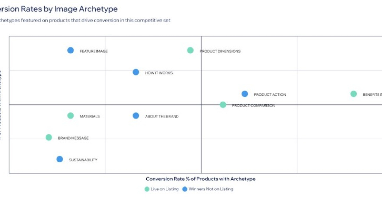
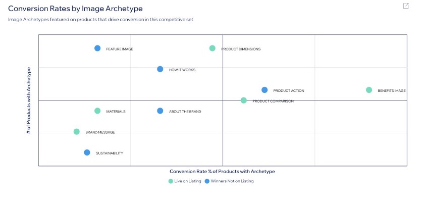
Content Brief analyzes consumer demographics, discovery behavior, and content performance to give brands a comprehensive understanding of their product’s position in the marketplace. What would normally require months of research and work is now done in minutes. Content Brief takes the guesswork out of product strategy with tools that do the heavy lifting. Its attribute importance ranking shows you which product features deserve the spotlight, and the image archetype analysis makes sure your visuals engage customers.
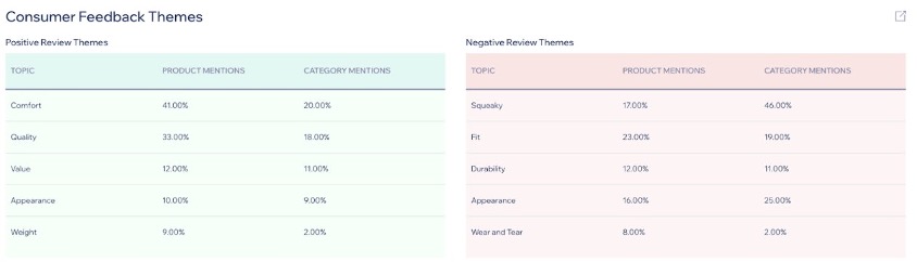
As shown in the following screenshot, the image archetype feature shows attributes that are driving sales in a given category, allowing brands to highlight the most impactful features in the image block and A+ image content.
Content Brief incorporates review and feedback analysis capabilities. It uses sentiment analysis to process customer reviews, identifying recurring themes in both positive and negative feedback, and highlights areas for potential improvement.
Content Brief’s Search Family analysis groups similar search terms together, helping brands understand distinct customer intent and tailor their content accordingly. This feature combined with detailed persona insights helps marketers create highly targeted content for specific segments. It also offers competitive analysis, providing side-by-side comparisons with competing products, highlighting areas where a brand’s product stands out or needs improvement.
“This is the thing we need the most as a business. We have all of the listening tools, review sentiment, keyword things, but nothing is in a single place like this and able to be optimized to my listing. And the thought of writing all those changes back to my PIM and then syndicating to all of my retailers, this is giving me goosebumps.”
– Marketing executive, Fortune 500 brand
Brands using Content Brief can more quickly identify opportunities for growth, adapt to change, and maintain a competitive edge in the digital marketplace. From search optimization and review analysis to competitive benchmarking and persona targeting, Content Brief empowers brands to create compelling, data-driven content that drives both traffic and conversions.
Select Brands looked to improve their Amazon performance and partnered with Pattern. Content Brief’s insights led to updates that caused a transformation for their Triple Buffet Server listing’s image stack. Their old image stack was created for marketplace requirements, whereas the new image stack was optimized with insights based on product attributes to highlight from category and sales data. The updated image stack featured bold product highlights and captured shoppers with lifestyle imagery. The results were a 21% MoM revenue surge, 14.5% more traffic, and a 21 bps conversion lift.
“Content Brief is a perfect example of why we chose to partner with Pattern. After just one month of testing, we see how impactful it can be for driving incremental growth—even on products that are already performing well. We have a product that, together with Pattern, we were able to grow into a top performer in its category in less than 2 years, and it’s exciting to see how adding this additional layer can grow revenue even for that product, which we already considered to be strong.”
– Eric Endres, President, Select Brands
To discover how Content Brief helped Select Brands boost their Amazon performance, refer to the full case study.
The AWS backbone of Content Brief
At the heart of Pattern’s architecture lies a carefully orchestrated suite of AWS services. Amazon Simple Storage Service (Amazon S3) serves as the cornerstone for storing product images, crucial for comprehensive ecommerce analysis. Amazon Textract is employed to extract and analyze text from these images, providing valuable insights into product presentation and enabling comparisons with competitor listings. Meanwhile, Amazon DynamoDB acts as the powerhouse behind Content Brief’s rapid data retrieval and processing capabilities, storing both structured and unstructured data, including content brief object blobs.
Pattern’s approach to data management is both innovative and efficient. As data is processed and analyzed, they create a shell in DynamoDB for each content brief, progressively injecting data as it’s processed and refined. This method allows for rapid access to partial results and enables further data transformations as needed, making sure that brands have access to the most up-to-date insights.
The following diagram illustrates the pipeline workflow and architecture.
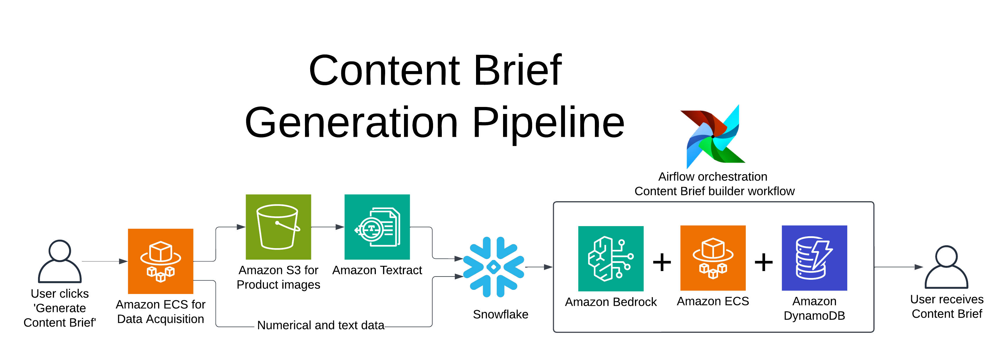
Scaling to handle 38 trillion data points
Processing over 38 trillion data points is no small feat, but Pattern has risen to the challenge with a sophisticated scaling strategy. At the core of this strategy is Amazon Elastic Container Store (Amazon ECS) with GPU support, which handles the computationally intensive tasks of natural language processing and data science. This setup allows Pattern to dynamically scale resources based on demand, providing optimal performance even during peak processing times.
To manage the complex flow of data between various AWS services, Pattern employs Apache Airflow. This orchestration tool manages the intricate dance of data with a primary DAG, creating and managing numerous sub-DAGs as needed. This innovative use of Airflow allows Pattern to efficiently manage complex, interdependent data processing tasks at scale.
But scaling isn’t just about processing power—it’s also about efficiency. Pattern has implemented batching techniques in their AI model calls, resulting in up to 50% cost reduction for two-batch processing while maintaining high throughput. They’ve also implemented cross-region inference to improve scalability and reliability across different geographical areas.
To keep a watchful eye on their system’s performance, Pattern employs LLM observability techniques. They monitor AI model performance and behavior, enabling continuous system optimization and making sure that Content Brief is operating at peak efficiency.
Using Amazon Bedrock for AI-powered insights
A key component of Pattern’s Content Brief solution is Amazon Bedrock, which plays a pivotal role in their AI and machine learning (ML) capabilities. Pattern uses Amazon Bedrock to implement a flexible and secure large language model (LLM) strategy.
Model flexibility and optimization
Amazon Bedrock offers support for multiple foundation models (FMs), which allows Pattern to dynamically select the most appropriate model for each specific task. This flexibility is crucial for optimizing performance across various aspects of Content Brief:
- Natural language processing – For analyzing product descriptions, Pattern uses models optimized for language understanding and generation.
- Sentiment analysis – When processing customer reviews, Amazon Bedrock enables the use of models fine-tuned for sentiment classification.
- Image analysis – Pattern currently uses Amazon Textract for extracting text from product images. However, Amazon Bedrock also offers advanced vision-language models that could potentially enhance image analysis capabilities in the future, such as detailed object recognition or visual sentiment analysis.
The ability to rapidly prototype on different LLMs is a key component of Pattern’s AI strategy. Amazon Bedrock offers quick access to a variety of cutting-edge models o facilitate this process, allowing Pattern to continuously evolve Content Brief and use the latest advancements in AI technology. Today, this allows the team to build seamless integration and use various state-of-the-art language models tailored to different tasks, including the new, cost-effective Amazon Nova models.
Prompt engineering and efficiency
Pattern’s team has developed a sophisticated prompt engineering process, continually refining their prompts to optimize both quality and efficiency. Amazon Bedrock offers support for custom prompts, which allows Pattern to tailor the model’s behavior precisely to their needs, improving the accuracy and relevance of AI-generated insights.
Moreover, Amazon Bedrock offers efficient inference capabilities that help Pattern optimize token usage, reducing costs while maintaining high-quality outputs. This efficiency is crucial when processing the vast amounts of data required for comprehensive ecommerce analysis.
Security and data privacy
Pattern uses the built-in security features of Amazon Bedrock to uphold data protection and compliance. By employing AWS PrivateLink, data transfers between Pattern’s virtual private cloud (VPC) and Amazon Bedrock occur over private IP addresses, never traversing the public internet. This approach significantly enhances security by reducing exposure to potential threats.
Furthermore, the Amazon Bedrock architecture makes sure that Pattern’s data remains within their AWS account throughout the inference process. This data isolation provides an additional layer of security and helps maintain compliance with data protection regulations.
“Amazon Bedrock’s flexibility is crucial in the ever-evolving landscape of AI, enabling Pattern to utilize the most effective and efficient models for their diverse ecommerce analysis needs. The service’s robust security features and data isolation capabilities give us peace of mind, knowing that our data and our clients’ information are protected throughout the AI inference process.”
– Jason Wells, CTO, Pattern
Building on Amazon Bedrock, Pattern has created a secure, flexible, and efficient AI-powered solution that continuously evolves to meet the dynamic needs of ecommerce optimization.
Conclusion
Pattern’s Content Brief demonstrates the power of AWS in revolutionizing data-driven solutions. By using services like Amazon Bedrock, DynamoDB, and Amazon ECS, Pattern processes over 38 trillion data points to deliver actionable insights, optimizing product listings across multiple services.
Inspired to build your own innovative, high-performance solution? Explore AWS’s suite of services at aws.amazon.com and discover how you can harness the cloud to bring your ideas to life. To learn more about how Content Brief could help your brand optimize its ecommerce presence, visit pattern.com.
About the Author
 Parker Bradshaw is an Enterprise SA at AWS who focuses on storage and data technologies. He helps retail companies manage large data sets to boost customer experience and product quality. Parker is passionate about innovation and building technical communities. In his free time, he enjoys family activities and playing pickleball.
How to configure cross-account model deployment using Amazon Bedrock Custom Model Import
In enterprise environments, organizations often divide their AI operations into two specialized teams: an AI research team and a model hosting team. The research team is dedicated to developing and enhancing AI models using model training and fine-tuning techniques. Meanwhile, a separate hosting team is responsible for deploying these models across their own development, staging, and production environments.
With Amazon Bedrock Custom Model Import, the hosting team can import and serve custom models using supported architectures such as Meta Llama 2, Llama 3, and Mistral using On-Demand pricing. Teams can import models with weights in Hugging Face safetensors format from Amazon SageMaker or from Amazon Simple Storage Service (Amazon S3). These imported custom models work alongside existing Amazon Bedrock foundation models (FMs) through a single, unified API in a serverless manner, alleviating the need to manage model deployment and scaling.
However, in such enterprise environments, these teams often work in separate AWS accounts for security and operational reasons. The model development team’s training results, known as model artifacts, for example model weights, are typically stored in S3 buckets within the research team’s AWS account, but the hosting team needs to access these artifacts from another account to deploy models. This creates a challenge: how do you securely share model artifacts between accounts?
This is where cross-account access becomes important. With Amazon Bedrock Custom Model Import cross-account support, we can help you configure direct access between the S3 buckets storing model artifacts and the hosting account. This streamlines your operational workflow while maintaining security boundaries between teams. One of our customers quotes:
Bedrock Custom Model Import cross-account support helped AI Platform team to simplify the configuration, reduce operational overhead and secure models in the original location.
– Scott Chang, Principal Engineer, AI Platform at Salesforce
In this guide, we walk you through step-by-step instructions for configuring cross-account access for Amazon Bedrock Custom Model Import, covering both non-encrypted and AWS Key Management Service (AWS KMS) based encrypted scenarios.
Example scenario
For this walkthrough, consider two AWS accounts:
- Model Development account (
111122223333):- Stores model artifacts (custom weights and configurations) in an S3 bucket called
model-artifacts-111122223333 - Optionally encrypts artifacts using AWS KMS customer managed key
kms-cmk-111122223333
- Stores model artifacts (custom weights and configurations) in an S3 bucket called
- Model Hosting account (
777788889999):- Hosts models using Amazon Bedrock Custom Model Import
- Uses a new AWS Identity and Access Management (IAM) execution role
BedrockCMIExecutionRole-777788889999 - Can optionally encrypt artifacts using AWS KMS key
kms-cmk-777788889999
The following figure illustrates this setup, showing how the cross-account access is configured between the S3 bucket, KMS keys, and Amazon Bedrock Custom Model Import.

To successfully implement the described scenario while adhering to the principle of least privilege access, the following steps must be executed:
- The Model Development account must provide access to the Model Hosting account’s IAM role
BedrockCMIExecutionRole-777788889999, allowing it to utilize their S3 bucket and, if applicable, the encryption key, using resource-based policies. - The Model Hosting account should establish an IAM role, such as
BedrockCMIExecutionRole-777788889999. The identity-based policies needed would be for the Model Development S3 bucket and customer managed keys for decrypting model artifacts, like usingkms-cmk-111122223333. - The Model Hosting account must enable the Amazon Bedrock service to assume the IAM role
BedrockCMIExecutionRole-777788889999, created in step 2, by including the Amazon Bedrock service as a trusted entity. This IAM role will be utilized by the Model Hosting account to initiate the custom model import job.
Prerequisites
Before you can start a custom model import job, you need to fulfill the following prerequisites:
- If you’re importing your model from an S3 bucket, prepare your model files in the Hugging Face weights format. For more information refer to Import source.
- (Optional) Set up extra security configurations.
- You can encrypt input and output data, import jobs, or inference requests made to imported models. For more information refer to Encryption of custom model import.
- You can create a virtual private cloud (VPC) to protect your customization jobs. For more information, refer to (Optional) Protect custom model import jobs using a VPC.
Step-by-step execution
The following section provides the step-by-step execution of the previously outlined high-level process, from the perspective of an administrator managing both accounts:
Step 1: Set up the S3 bucket policy (in the Model Development account) to enable access for the Model Hosting account’s IAM role:
- Sign in to the AWS Management Console for account
111122223333, then access the Amazon S3 console. - On the General purpose buckets view, locate
model-artifacts-111122223333, the bucket used by the model development team to store their model artifacts. - On the Permissions tab, select Edit in the Bucket policy section, and insert the following IAM resource-based policy. Be sure to update the AWS account IDs (shown in red) in the policy with your information.
Step 2: Establish an IAM role (in the Model Hosting account) and authorize Amazon Bedrock to assume this role:
- Sign in to the AWS console for account
777788889999and launch the IAM console. - In the left navigation pane, select Policies and then choose Create policy. Within the Policy Editor, switch to the JSON tab and insert the following identity-based policy. This policy is designed for read-only access, enabling users or a role to list and download objects from a specified S3 bucket, but only if the bucket is owned by account
111122223333. Customize the AWS account ID and S3 bucket name/prefix (shown in red) with your information.
- Choose Next, assign the policy name as
BedrockCMIExecutionPolicy-777788889999, and finalize by choosing Create policy. - In the left navigation pane, choose Roles and select Custom trust policy as the Trusted entity type. Insert the following trusted entity policy, which restricts the role assumption to the Amazon Bedrock service, specifically for model import jobs in account
777788889999located in the US East (N. Virginia)us-east-1Region. Modify the AWS account ID and Region (shown in red) with your information.
- Choose Next and in the Add permissions section, search for the policy created in the previous step
BedrockCMIExecutionPolicy-777788889999, select the checkbox, and proceed by choosing Next. - Assign the Role name as
BedrockCMIExecutionRole-777788889999, provide a Description as “IAM execution role to be used by CMI jobs,” and finalize by choosing Create role.
Important: If you’re using an AWS KMS encryption key for model artifacts in the Model Development account or for imported model artifacts with the Amazon Bedrock managed AWS account, proceed with steps 3 through 5. If not, skip to step 6.
Step 3: Adjust the AWS KMS key policy (in the Model Development account) to allow the Amazon Bedrock CMI execution IAM role to decrypt model artifacts:
- Transition back to the Model Development account and find the AWS KMS key named
kms-cmk-111122223333in the AWS KMS console. Note the AWS KMS key Amazon Resource Name (ARN). - On the Key policy tab, switch to the Policy view, and incorporate the following resource-based policy statement to enable the Model Hosting account’s IAM role
BedrockCMIExecutionRole-777788889999to decrypt model artifacts. Revise items in red with your information.
Step 4: Set the AWS KMS key policy (in the Model Hosting account) for the CMI execution IAM role to encrypt and decrypt model artifacts to securely store in the Amazon Bedrock AWS account:
- Return to the Model Hosting account and locate the AWS KMS key named
kms-cmk-777788889999in the AWS KMS console. Note the AWS KMS key ARN. - Insert the following statement into the AWS KMS key’s resource-based policy to enable the
BedrockCMIExecutionRole-777788889999IAM role to encrypt and decrypt model artifacts at rest in the Amazon Bedrock managed AWS account. Revise items in red with your information.
Step 5: Modify the CMI execution role’s permissions (in the Model Hosting account) to provide access to encryption keys:
Access the IAM console and find the IAM policy BedrockCMIExecutionPolicy-777788889999. To the existing identity-based policy, append the following statements (replace the ARNs in red with one noted in steps 4 and 5):
Step 6: Initiate the Model import job (in the Model Hosting account)
In this step, we execute the model import job using the AWS Command Line Interface (AWS CLI) command. You can also use AWS SDKs or APIs for the same purpose. Run the following command from your terminal session with an IAM user or role that has the necessary privileges to create a custom model import job. You don’t need to explicitly provide an ARN or details of the CMK used by the Model Development team.
When encrypting model artifacts with Amazon Bedrock Custom Model Import, use the --imported-model-kms-key-id flag and specify the ARN of the Model Hosting account’s CMK key.
Cross-account access to the S3 bucket using the custom model import job is only supported through AWS CLI, AWS SDKs, or APIs. Console support is not yet available.
Troubleshooting
When IAM policy misconfigurations prevent a custom model import job, you might encounter an error like:
To resolve this, manually verify access to Model Development’s S3 bucket from the Model Hosting account by assuming the BedrockCMIExecutionRole-777788889999. Follow these steps:
Step 1: Identify the current IAM role or user in the CLI with the following and copy the ARN from the output:
Step 2: Update trust relationships. Append the trust policy of the BedrockCMIExecutionRole-777788889999 to allow the current user or IAM role to assume this role:
Step 3: List or copy the S3 bucket contents assuming the Amazon Bedrock Custom Model Import execution role
- Assume the CMI execution role (replace the ARN with your information):
- Export the returned temporary credentials as environment variables:
- Run commands to troubleshoot permission issues:
If errors persist, consider using Amazon Q Developer or refer to additional resources outlined in the IAM User Guide.
Cleanup
There is no additional charge to import a custom model to Amazon Bedrock (refer to step 6 in the Step-by-step execution section). However, if your model isn’t in use for inference, and you want to avoid paying storage costs (refer to Amazon Bedrock pricing), delete the imported model using the AWS console or AWS CLI reference or API Reference. For example (replace the text in red with your imported model name):
Conclusion
By using cross-account access in Amazon Bedrock Custom Model Import, organizations can significantly streamline their AI model deployment workflows.
Amazon Bedrock Custom Model Import is generally available today in Amazon Bedrock in the US East (N. Virginia) us-east-1 and US West (Oregon) us-west-2 AWS Regions. Refer to the full Region list for future updates. To learn more, refer to the Amazon Bedrock Custom Model Import product page and Amazon Bedrock pricing page. Give Amazon Bedrock Custom Model Import a try in the Amazon Bedrock console today and send feedback to AWS re:Post for Amazon Bedrock or through your usual AWS Support contacts.
Thank you to our contributors Scott Chang (Salesforce), Raghav Tanaji (Salesforce), Rupinder Grewal (AWS), Ishan Singh (AWS), and Dharinee Gupta (AWS)
About the Authors
 Hrushikesh Gangur is a Principal Solutions Architect at AWS. Based in San Francisco, California, Hrushikesh is an expert in AWS machine learning. As a thought leader in the field of generative AI, Hrushikesh has contributed to AWS’s efforts in helping startups and ISVs build and deploy AI applications. His expertise extends to various AWS services, including Amazon SageMaker, Amazon Bedrock, and accelerated computing which are crucial for building AI applications.
 Sai Darahas Akkineni is a Software Development Engineer at AWS. He holds a master’s degree in Computer Engineering from Cornell University, where he worked in the Autonomous Systems Lab with a specialization in computer vision and robot perception. Currently, he helps deploy large language models to optimize throughput and latency.
 Prashant Patel is a Senior Software Development Engineer in AWS. He’s passionate about scaling large language models for enterprise applications. Prior to joining AWS, he worked at IBM on productionizing large-scale AI/ML workloads on Kubernetes. Prashant has a master’s degree from NYU Tandon School of Engineering. While not at work, he enjoys traveling and playing with his dogs.
ByteDance processes billions of daily videos using their multimodal video understanding models on AWS Inferentia2
This is a guest post authored by the team at ByteDance.
ByteDance is a technology company that operates a range of content platforms to inform, educate, entertain, and inspire people across languages, cultures, and geographies. Users trust and enjoy our content platforms because of the rich, intuitive, and safe experiences they provide. These experiences are made possible by our machine learning (ML) backend engine, with ML models built for video understanding, search, recommendation, advertising, and novel visual effects.
In support of its mission to “Inspire Creativity and Enrich Life,” we’ve made it straightforward and fun for people to engage with, create, and consume content. People can also discover and transact with a suite of more than a dozen products and services, such as CapCut, e-Shop, Lark, Pico, and Mobile Legends: Bang Bang.
At ByteDance, we collaborated with Amazon Web Services (AWS) to deploy multimodal large language models (LLMs) for video understanding using AWS Inferentia2 across multiple AWS Regions around the world. By using sophisticated ML algorithms, the platform efficiently scans billions of videos each day. We use this process to identify and flag content that violates community guidelines, enabling a better experience for all users. By using Amazon EC2 Inf2 instances for these video understanding workloads, we were able to cut the inference cost by half.
In this post, we discuss the use of multimodal LLMs for video understanding, the solution architecture, and techniques for performance optimization.
Overcoming video understanding hurdles with multimodal LLMs
Multimodal LLMs enable better understanding of the world, enabling various forms of digital content as inputs to the LLM, greatly increasing the range of useful applications we can now build. The need for AI systems capable of processing various content forms has become increasingly apparent. Multimodal LLMs have risen to meet this challenge by taking multiple data modalities, including text, images, audio, and video (refer to the following diagram), which allows for full understanding of content, mimicking human perception and interaction with the world. The enhanced capabilities of these models are evident in their performance, which far surpasses that of traditional models in tasks ranging from sophisticated virtual assistant to advanced content creation. By expanding the boundaries of AI capabilities and paving the way for more natural and intuitive interactions with technology, these models aren’t just improving existing applications but opening doors to entirely new possibilities in the realm of AI and user experience.

In our operations, the implementation of multimodal LLMs for video understanding represents a significant shift in thinking about AI-driven content analysis. This innovation addresses the daily challenge of processing billions of volumes of video content, overcoming the efficiency limits of traditional AI models. We’ve developed our own multimodal LLM architecture, designed to achieve state-of-the-art performance across single-image, multi-image, and video applications. Unlike traditional ML models, this new generative AI–enabled system integrates multiple input streams into a unified representational space. Cross-modal attention mechanisms facilitate information exchange between modalities, and fusion layers combine representations from different modalities. The decoder then generates output based on the fused multimodal representation, enabling a more nuanced and context-aware analysis of content.
Solution overview
We’ve collaborated with AWS since the first generation of Inferentia chips. Our video understanding department has been committed to finding more cost-efficient solutions that deliver higher performance to better meet ever-growing business needs. During this period, we found that AWS has been continually inventing and adding features and capabilities to its AWS Neuron software development kit (SDK), the software enabling high-performance workloads on the Inferentia chips. The popular Meta Llama and Mistral models were well supported with high performance on Inferentia2 shortly after their open source release. Therefore, we began to evaluate the Inferentia2 based solution, illustrated in the following diagram.

We made the strategic decision to deploy a fine-tuned middle-sized LLM on Inferentia2, to provide a performant and cost-effective solution capable of processing billions of videos daily. The process was a comprehensive effort aimed at optimizing end-to-end response time for our video understanding workload. The team explored a wide range of parameters, including tensor parallel sizes, compile configurations, sequence lengths, and batch sizes. We employed various parallelization techniques, such as multi-threading and model replication (for non-LLM models) across multiple NeuronCores. Through these optimizations, which included parallelizing sequence steps, reusing devices, and using auto-benchmark and profiling tools, we achieved a substantial performance boost, maintaining our position at the forefront of industry performance standards
We used tensor parallelism to effectively distribute and scale the model across multiple accelerators in an Inf2 instance. We used static batching, which improved the latency and throughput of our models by making sure that data is processed in uniform, fixed-size batches during inference. Using repeated n-grams filtering significantly improved the quality of automatically generated text and reduced inference time. Quantizing the weights of the multimodal model from FP16/BF16 to INT8 format allowed it to run more efficiently on Inferentia2 with less device memory usage, without compromising on accuracy. Using these techniques and model serialization, we optimized the throughput on inf2.48xlarge instance by maximizing the batch size such that the model could still fit on a single accelerator in an instance so we could deploy multiple model replicas on the same instance. This comprehensive optimization strategy helped us meet our latency requirements while providing optimal throughput and cost reduction. Notably, the Inferentia2 based solution cut the cost by half compared to comparable Amazon Elastic Compute Cloud (Amazon EC2) instances, highlighting the significant economic advantages of using Inferentia2 chips for large-scale video understanding tasks.
The following diagram shows how we deploy our LLM container on Amazon EC2 Inf2 instances using Neuron.

In summary, our collaboration with AWS has revolutionized video understanding, setting new industry standards for efficiency and accuracy. The multimodal LLM’s ability to adapt to global market demands and its scalable performance on Inferentia2 chips underscore the profound impact of this technology in safeguarding the platform’s global community.
Future plans
Looking further ahead, the development of a unified multimodal LLM represents an important shift in video understanding technology. This ambitious project aims to create a universal content tokenizer capable of processing all content types and aligning them within a common semantic space. After it’s tokenized, the content will be analyzed by advanced large models, generating appropriate content understanding outputs regardless of the original format (as shown in the following diagram). This unified approach can streamline the content understanding process, potentially improving both efficiency and consistency across diverse content types.

For additional learning, refer to the paper The Evolution of Multimodal Model Architectures.
The implementation of this comprehensive strategy sets new benchmarks in video understanding technology, striking a balance between accuracy, speed, and cultural sensitivity in an increasingly complex digital ecosystem. This forward-looking approach not only addresses current challenges in video understanding but also positions the system at the forefront of AI-driven content analysis and management for the foreseeable future.
By using cutting-edge AI techniques and a holistic approach to content understanding, this next-generation content understanding system aims to set new industry standards, providing safer and more inclusive online environments while adapting to the ever-evolving landscape of digital communication. At the same time, AWS is investing in next-generation AI chips such as AWS Trainium2, which will continue to push the performance boundaries while keeping costs under control. At ByteDance, we’re planning to test out this new generation of AWS AI chips and adopt them appropriately as the models and workloads continue to evolve.
Conclusion
The collaboration between ByteDance and AWS has revolutionized video understanding through the deployment of multimodal LLMs on Inferentia2 chips. This partnership has yielded remarkable results, the ability to process billions of videos daily, and significant cost reductions and higher performance over comparable EC2 instances.
As ByteDance continues to innovate with projects such as the unified multimodal large model, we remain committed to pushing the boundaries of AI-driven content analysis. Our goal is to make sure our platforms remain safe, inclusive, and creative spaces for our global community, setting new industry standards for efficient video understanding.
To learn more about Inf2 instances, refer to Amazon EC2 Inf2 Architecture.
About the Authors
 Wangpeng An, Principal Algorithm Engineer at TikTok, specializes in multimodal LLMs for video understanding, advertising, and recommendations. He has led key projects in model acceleration, content moderation, and Ads LLM pipelines, enhancing TikTok’s real-time machine learning systems.
 Haotian Zhang is a Tech Lead MLE at TikTok, specializing in content understanding, search, and recommendation. He received an ML PhD from University of Waterloo. At TikTok, he leads a group of engineers to improve the efficiency, robustness, and effectiveness of training and inference for LLMs and multimodal LLMs, especially for large distributed ML systems.
 Xiaojie Ding is a senior engineer at TikTok, focusing on content moderation system development, model resource and deployment optimization, and algorithm engineering stability construction. In his free time, he likes to play single-player games.
 Nachuan Yang is a senior engineer at TikTok, focusing on content security and moderation. He has successively been engaged in the construction of moderation systems, model applications, and deployment and performance optimization.
 Kairong Sun is a Senior SRE on the AML Team at ByteDance. His role focuses on maintaining the seamless operation and efficient allocation of resources within the cluster, specializing in cluster machine maintenance and resource optimization.
The authors would like to thank other ByteDance and AWS team members for their contributions: Xi Dai, Kaili Zhao, Zhixin Zhang, Jin Ye, and Yann Xia from ByteDance; Jia Dong, Bingyang Huang, Kamran Khan, Shruti Koparkar, and Diwakar Bansal from AWS.
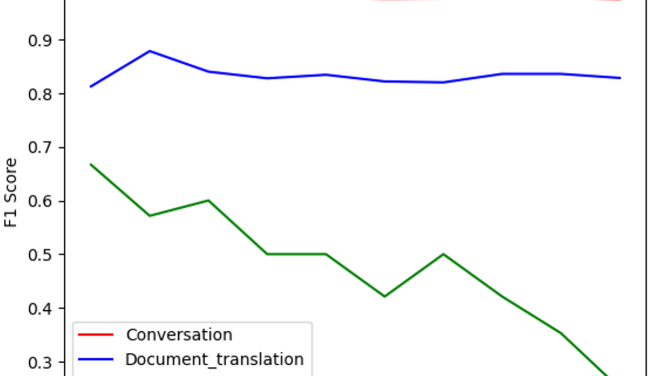
How IDIADA optimized its intelligent chatbot with Amazon Bedrock
This post is co-written with Xavier Vizcaino, Diego Martín Montoro, and Jordi Sánchez Ferrer from Applus+ Idiada.
In 2021, Applus+ IDIADA, a global partner to the automotive industry with over 30 years of experience supporting customers in product development activities through design, engineering, testing, and homologation services, established the Digital Solutions department. This strategic move aimed to drive innovation by using digital tools and processes. Since then, we have optimized data strategies, developed customized solutions for customers, and prepared for the technological revolution reshaping the industry.
AI now plays a pivotal role in the development and evolution of the automotive sector, in which Applus+ IDIADA operates. Within this landscape, we developed an intelligent chatbot, AIDA (Applus Idiada Digital Assistant)— an Amazon Bedrock powered virtual assistant serving as a versatile companion to IDIADA’s workforce.
Amazon Bedrock is a fully managed service that offers a choice of high-performing foundation models (FMs) from leading AI companies like AI21 Labs, Anthropic, Cohere, Meta, Stability AI, and Amazon through a single API, along with a broad set of capabilities to build generative AI applications with security, privacy, and responsible AI.
With Amazon Bedrock, AIDA assists with a multitude of tasks, from addressing inquiries to tackling complex technical challenges spanning code, mathematics, and translation. Its capabilities are truly boundless.
With AIDA, we take another step towards our vision of providing global and integrated digital solutions that add value for our customers. Its internal deployment strengthens our leadership in developing data analysis, homologation, and vehicle engineering solutions. Additionally, in the medium term, IDIADA plans to offer AIDA as an integrable product for customers’ environments and develop “light” versions seamlessly integrable into existing systems.
In this post, we showcase the research process undertaken to develop a classifier for human interactions in this AI-based environment using Amazon Bedrock. The objective was to accurately identify the type of interaction received by the intelligent agent to route the request to the appropriate pipeline, providing a more specialized and efficient service.
The challenge: Optimize intelligent chatbot responses, allocate resources more effectively, and enhance the overall user experience
Built on a flexible and secure architecture, AIDA offers a versatile environment for integrating multiple data sources, including structured data from enterprise databases and unstructured data from internal sources like Amazon Simple Storage Service (Amazon S3). It boasts advanced capabilities like chat with data, advanced Retrieval Augmented Generation (RAG), and agents, enabling complex tasks such as reasoning, code execution, or API calls.
As AIDA’s interactions with humans proliferated, a pressing need emerged to establish a coherent system for categorizing these diverse exchanges.
Initially, users were making simple queries to AIDA, but over time, they started to request more specific and complex tasks. These included document translations, inquiries about IDIADA’s internal services, file uploads, and other specialized requests.
The main reason for this categorization was to develop distinct pipelines that could more effectively address various types of requests. By sorting interactions into categories, AIDA could be optimized to handle specific kinds of tasks more efficiently. This approach allows for tailored responses and processes for different types of user needs, whether it’s a simple question, a document translation, or a complex inquiry about IDIADA’s services.
The primary objective is to offer a more specialized service through the creation of dedicated pipelines for various contexts, such as conversation, document translation, and services to provide more accurate, relevant, and efficient responses to users’ increasingly diverse and specialized requests.
Solution overview
By categorizing the interactions into three main groups—conversation, services, and document translation—the system can better understand the user’s intent and respond accordingly. The Conversation class encompasses general inquiries and exchanges, the Services class covers requests for specific functionalities or support, and the Document_Translation class handles text translation needs.
The specialized pipelines, designed specifically for each use case, allow for a significant increase in efficiency and accuracy of AIDA’s responses. This is achieved in several ways:
- Enhanced efficiency – By having dedicated pipelines for specific types of tasks, AIDA can process requests more quickly. Each pipeline is optimized for its particular use case, which reduces the computation time needed to generate an appropriate response.
- Increased accuracy – The specialized pipelines are equipped with specific tools and knowledge for each type of task. This allows AIDA to provide more accurate and relevant responses, because it uses the most appropriate resources for each type of request.
- Optimized resource allocation – By classifying interactions, AIDA can allocate computational resources more efficiently, directing the appropriate processing power to each type of task.
- Improved response time – The combination of greater efficiency and optimized resource allocation results in faster response times for users.
- Enhanced adaptability – This system allows AIDA to better adapt to different types of requests, from simple queries to complex tasks such as document translations or specialized inquiries about IDIADA services.
The research and development of this large language model (LLM) based classifier is an important step in the continuous improvement of the intelligent agent’s capabilities within the Applus IDIADA environment.
For this occasion, we use a set of 1,668 examples of pre-classified human interactions. These have been divided into 666 for training and 1,002 for testing. A 40/60 split has been applied, giving significant importance to the test set.
The following table shows some examples.
| SAMPLE | CLASS |
| Can you make a summary of this text? “Legislation for the Australian Government’s …” | Conversation |
| No, only focus on this sentence : Braking technique to enable maximum brake application speed | Conversation |
| In a factory give me synonyms of a limiting resource of activities | Conversation |
| We need a translation of the file “Company_Bylaws.pdf” into English, could you handle it? | Document_Translation |
| Please translate the file “Product_Manual.xlsx” into English | Document_Translation |
| Could you convert the document “Data_Privacy_Policy.doc’ into English, please? | Document_Translation |
| Register my username in the IDIADA’s human resources database | Services |
| Send a mail to random_user@mail.com to schedule a meeting for the next weekend | Services |
| Book an electric car charger for me at IDIADA | Services |
We present three different classification approaches: two based on LLMs and one using a classic machine learning (ML) algorithm. The aim is to understand which approach is most suitable for addressing the presented challenge.
LLM-based classifier: Simple prompt
In this case, we developed an LLM-based classifier to categorize inputs into three classes: Conversation, Services, and Document_Translation. Instead of relying on predefined, rigid definitions, our approach follows the principle of understanding a set. This principle involves analyzing the common characteristics and patterns present in the examples or instances that belong to each class. By studying the shared traits of inputs within a class, we can derive an understanding of the class itself, without being constrained by preconceived notions.
It’s important to note that the learned definitions might differ from common expectations. For instance, the Conversation class encompasses not only typical conversational exchanges but also tasks like text summarization, which share similar linguistic and contextual traits with conversational inputs.
By following this data-driven approach, the classifier can accurately categorize new inputs based on their similarity to the learned characteristics of each class, capturing the nuances and diversity within each category.
The code consists of the following key components: libraries, a prompt, model invocation, and an output parser.
Libraries
The programming language used in this code is Python, complemented by the LangChain module, which is specifically designed to facilitate the integration and use of LLMs. This module provides a comprehensive set of tools and abstractions that streamline the process of incorporating and deploying these advanced AI models.
To take advantage of the power of these language models, we use Amazon Bedrock. The integration with Amazon Bedrock is achieved through the Boto3 Python module, which serves as an interface to the AWS, enabling seamless interaction with Amazon Bedrock and the deployment of the classification model.
Prompt
The task is to assign one of three classes (Conversation, Services, or Document_Translation) to a given sentence, represented by question:
- Conversation class – This class encompasses casual messages, summarization requests, general questions, affirmations, greetings, and similar types of text. It also includes requests for text translation, summarization, or explicit inquiries about the meaning of words or sentences in a specific language.
- Services class – Texts belonging to this class consist of explicit requests for services such as room reservations, hotel bookings, dining services, cinema information, tourism-related inquiries, and similar service-oriented requests.
- Document_Translation class – This class is characterized by requests for the translation of a document to a specific language. Unlike the
Conversationclass, these requests don’t involve summarization. Additionally, the name of the document to be translated and the target language are specified.
The prompt suggests a hierarchical approach to the classification process. First, the sentence should be evaluated to determine if it can be classified as a conversation. If the sentence doesn’t fit the Conversation class, one of the other two classes (Services or Document_Translation) should be assigned.
The priority for the Conversation class stems from the fact that 99% of the interactions are actually simple questions regarding various matters.
Model invocation
We use Anthropic’s Claude 3 Sonnet model for the natural language processing task. This LLM model has a context window of 200,000 tokens, enabling it to manage different languages and retrieve highly accurate answers. We use two key parameters:
- max_tokens – This parameter limits the maximum number of tokens (words or subwords) that the language model can generate in its output to 50.
- temperature – This parameter controls the randomness of the language model’s output. A temperature of 0.0 means that the model will produce the most likely output according to its training, without introducing randomness.
Output parser
Another important component is the output parser, which allows us to gather the desired information in JSON format. To achieve this, we use the LangChain parameter output_parsers.
The following code illustrates a simple prompt approach:
LLM-based classifier: Example augmented inference
We use RAG techniques to enhance the model’s response capabilities. Instead of relying solely on compressed definitions, we provide the model with a quasi-definition by extension. Specifically, we present the model with a diverse set of examples for each class, allowing it to learn the inherent characteristics and patterns that define each category. For instance, in addition to a concise definition of the Conversation class, the model is exposed to various conversational inputs, enabling it to identify common traits such as informal language, open-ended questions, and back-and-forth exchanges. This example-driven approach complements the initial descriptions provided, allowing the model to capture the nuances and diversity within each class. By combining concise definitions with representative examples, the RAG technique helps the model develop a more comprehensive understanding of the classes, enhancing its ability to accurately categorize new inputs based on their inherent nature and characteristics.
The following code provides examples in JSON format for RAG:
The total number of examples provided for each class is as follows:
- Conversation – 500 examples. This is the most common class, and only 500 samples are given to the model due to the vast amount of information, which could cause infrastructure overflow (very high delays, throttling, connection shutouts). This is a crucial point to note because it represents a significant bottleneck. Providing more examples to this approach could potentially improve performance, but the question remains: How many examples? Surely, a substantial amount would be required.
- Services – 26 examples. This is the least common class, and in this case, all available training data has been used.
- Document_Translation – 140 examples. Again, all available training data has been used for this class.
One of the key challenges with this approach is scalability. Although the model’s performance improves with more training examples, the computational demands quickly become overwhelming for our current infrastructure. The sheer volume of data required can lead to quota issues with Amazon Bedrock and unacceptably long response times. Rapid response times are essential for providing a satisfactory user experience, and this approach falls short in that regard.
In this case, we need to modify the code to embed all the examples. The following code shows the changes applied to the first version of the classifier. The prompt is modified to include all the examples in JSON format under the “Here you have some examples” section.
K-NN-based classifier: Amazon Titan Embeddings
In this case, we take a different approach by recognizing that despite the multitude of possible interactions, they often share similarities and repetitive patterns. Instead of treating each input as entirely unique, we can use a distance-based approach like k-nearest neighbors (k-NN) to assign a class based on the most similar examples surrounding the input. To make this work, we need to transform the textual interactions into a format that allows algebraic operations. This is where embeddings come into play. Embeddings are vector representations of text that capture semantic and contextual information. We can calculate the semantic similarity between different interactions by converting text into these vector representations and comparing their vectors and determining their proximity in the embedding space.
To accommodate this approach, we need to modify the code accordingly:
We used the Amazon Titan Text Embeddings G1 model, which generates vectors of 1,536 dimensions. This model is trained to accept multiple languages while retaining the semantic meaning of the embedded phrases.
For the classfier, we employed a classic ML algorithm, k-NN, using the scikit-learn Python module. This method takes a parameter, which we set to 3.
The following figure illustrates the F1 scores for each class plotted against the number of neighbors (k) used in the k-NN algorithm. As the graph shows, the optimal value for k is 3, which yields the highest F1 score for the most prevalent class, Document_Translation. Although it’s not the absolute highest score for the Services class, Document_Translation is significantly more common, making k=3 the best overall choice to maximize performance across all classes.
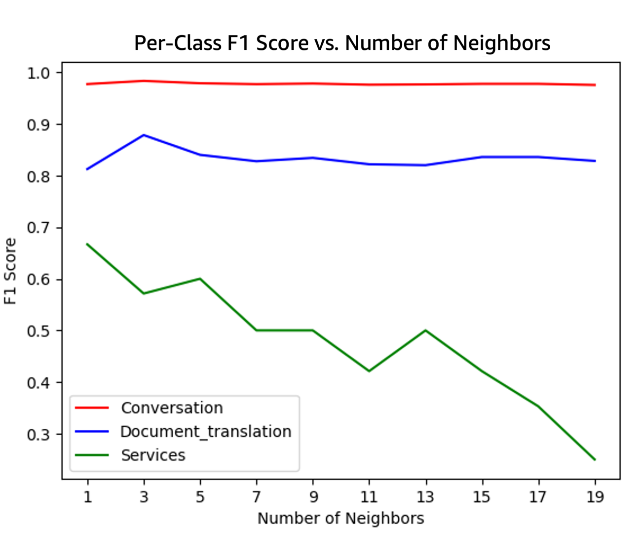
K-NN-based classifier: Cohere’s multilingual embeddings model
In the previous section, we used the popular Amazon Titan Text Embeddings G1 model to generate text embeddings. However, other models might offer different advantages. In this section, we explore the use of Cohere’s multilingual model on Amazon Bedrock for generating embeddings. We chose the Cohere model due to its excellent capability in handling multiple languages without compromising the vectorization of phrases. As we will demonstrate, this model doesn’t introduce significant differences in the generated vectors compared to other models, making it more suitable for use in a multilingual environment like AIDA.
To use the Cohere model, we need to change the model_id:
We use Cohere’s multilingual embeddings model to generate vectors with 1,024 dimensions. This model is trained to accept multiple languages and retain the semantic meaning of the embedded phrases.
For the classifier, we employ k-NN, using the scikit-learn Python module. This method takes a parameter, which we have set to 11.
The following figure illustrates the F1 scores for each class plotted against the number of neighbors used. As depicted, the optimal point is k=11, achieving the highest value for Document_Translation and the second-highest for Services. In this instance, the trade-off between Documents_Translation and Services is favorable.
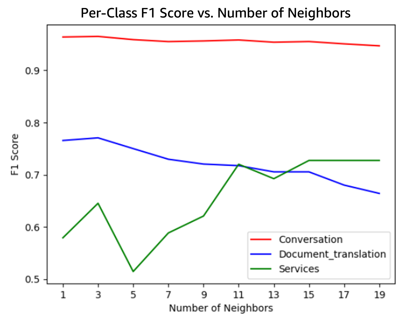
Amazon Titan Embeddings vs. Cohere’s multilingual embeddings model
In this section, we delve deeper into the embeddings generated by both models, aiming to understand their nature and consequently comprehend the results obtained. To achieve this, we have performed dimensionality reduction to visualize the vectors obtained in both cases in 2D.
Cohere’s multilingual embeddings model has a limitation on the size of the text it can vectorize, posing a significant constraint. Therefore, in the implementation showcased in the previous section, we applied a filter to only include interactions up to 1,500 characters (excluding cases that exceed this limit).
The following figure illustrates the vector spaces generated in each case.
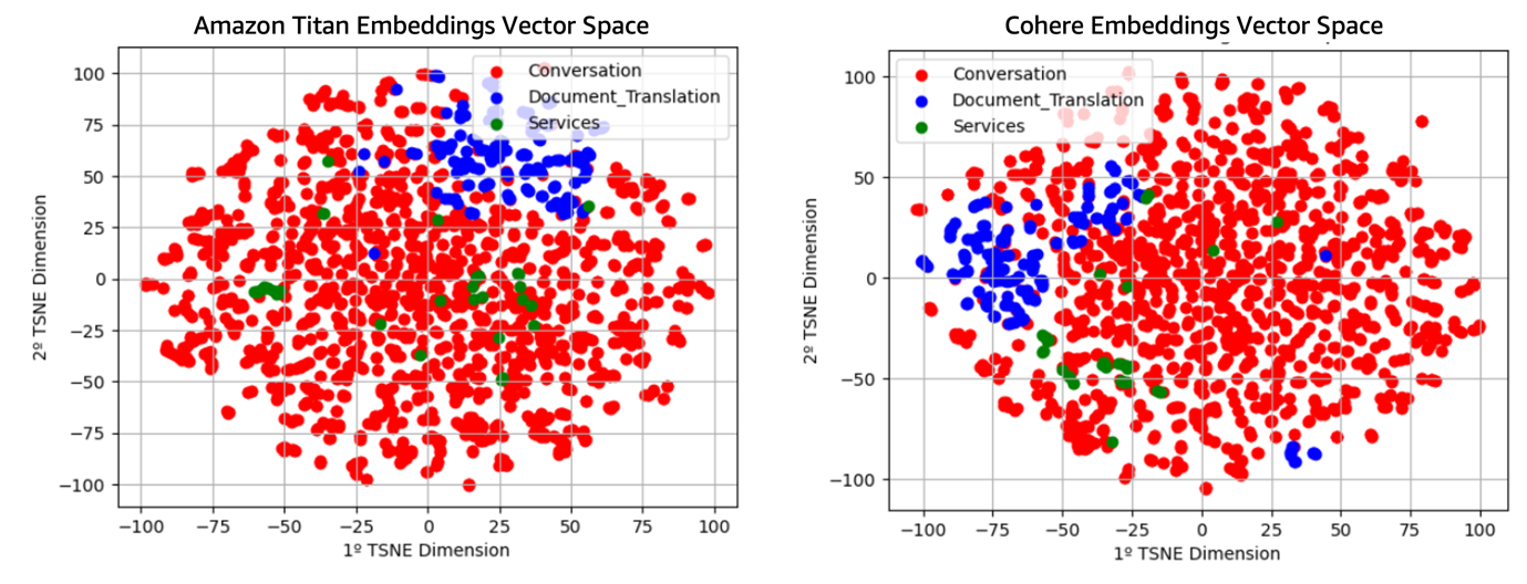
As we can observe, the generated vector spaces are relatively similar, initially appearing to be analogous spaces with a rotation between one another. However, upon closer inspection, it becomes evident that the direction of maximum variance in the case of Cohere’s multilingual embeddings model is distinct (deducible from observing the relative position and shape of the different groups). This type of situation, where high class overlap is observed, presents an ideal case for applying algorithms such as k-NN.
As mentioned in the introduction, most human interactions with AI are very similar to each other within the same class. This would explain why k-NN-based models outperform LLM-based models.
SVM-based classifier: Amazon Titan Embeddings
In this scenario, it is likely that user interactions belonging to the three main categories (Conversation, Services, and Document_Translation) form distinct clusters or groups within the embedding space. Each category possesses particular linguistic and semantic characteristics that would be reflected in the geometric structure of the embedding vectors. The previous visualization of the embeddings space displayed only a 2D transformation of this space. This doesn’t imply that clusters coudn’t be highly separable in higher dimensions.
Classification algorithms like support vector machines (SVMs) are especially well-suited to use this implicit geometry of the data. SVMs seek to find the optimal hyperplane that separates the different groups or classes in the embedding space, maximizing the margin between them. This ability of SVMs to use the underlying geometric structure of the data makes them an intriguing option for this user interaction classification problem.
Furthermore, SVMs are a robust and efficient algorithm that can effectively handle high-dimensional datasets, such as text embeddings. This makes them particularly suitable for this scenario, where the embedding vectors of the user interactions are expected to have a high dimensionality.
The following code illustrates the implementation:
We use Amazon Titan Text Embeddings G1. This model generates vectors of 1,536 dimensions, and is trained to accept several languages and to retain the semantic meaning of the phrases embedded.
To implement the classifier, we employed a classic ML algorithm, SVM, using the scikit-learn Python module. The SVM algorithm requires the tuning of several parameters to achieve optimal performance. To determine the best parameter values, we conducted a grid search with 10-fold cross-validation, using the F1 multi-class score as the evaluation metric. This systematic approach allowed us to identify the following set of parameters that yielded the highest performance for our classifier:
- C – We set this parameter to 1. This parameter controls the trade-off between allowing training errors and forcing rigid margins. It acts as a regularization parameter. A higher value of C (for example, 10) indicates a higher penalty for misclassification errors. This results in a more complex model that tries to fit the training data more closely. A higher C value can be beneficial when the classes in the data are well separated, because it allows the algorithm to create a more intricate decision boundary to accurately classify the samples. On the other hand, a C value of 1 indicates a reasonable balance between fitting the training set and the model’s generalization ability. This value might be appropriate when the data has a simple structure, and a more flexible model isn’t necessary to capture the underlying relationships. In our case, the selected C value of 1 suggests that the data has a relatively simple structure, and a balanced model with moderate complexity is sufficient for accurate classification.
- class_weight – We set this parameter to
None. This parameter adjusts the weights of each class during the training process. Settingclass_weighttobalancedautomatically adjusts the weights inversely proportional to the class frequencies in the input data. This is particularly useful when dealing with imbalanced datasets, where one class is significantly more prevalent than the others. In our case, the value ofNonefor theclass_weightparameter suggests that the minor classes don’t have much relevance or impact on the overall classification task. This choice implies that the implicit geometry or decision boundaries learned by the model might not be optimized for separating the different classes effectively. - Kernel – We set this parameter to
linear. This parameter specifies the type of kernel function to be used by the SVC algorithm. Thelinearkernel is a simple and efficient choice because it assumes that the decision boundary between classes can be represented by a linear hyperplane in the feature space. This value suggests that, in a higher dimension vector space, the categories could be linearly separated by an hyperplane.
SVM-based classifier: Cohere’s multilingual embeddings model
The implementation details of the classifier are presented in the following code:
We use the Amazon Titan Text Embeddings G1 model, which generates vectors of 1,536 dimensions. This model is trained to accept multiple languages and retain the semantic meaning of the embedded phrases.
For the classifier, we employ SVM, using the scikit-learn Python module. To obtain the optimal parameters, we performed a grid search with 10-fold cross-validation based on the multi-class F1 score, resulting in the following selected parameters (as detailed in the previous section):
- C – We set this parameter to 1, which indicates a reasonable balance between fitting the training set and the model’s generalization ability. This setting suggests that the data has a simple structure and that a more flexible model might not be necessary to capture the underlying relationships.
- class_weight – We set this parameter to
None. A value ofNonesuggests that the minor classes don’t have much relevance, which in turn implies that the implicit geometry might not be suitable for separating the different classes. - kernel – We set this parameter to
linear. This value suggests that in a higher-dimensional vector space, the categories could be linearly separated by a hyperplane.
ANN-based classifier: Amazon Titan and Cohere’s multilingual embeddings model
Given the promising results obtained with SVMs, we decided to explore another geometry-based method by employing an Artificial Neural Network (ANN) approach.
In this case, we performed normalization of the input vectors to use the advantages of normalization when using neural networks. Normalizing the input data is a crucial step when working with ANNs, because it can help improve the model’s during training. We applied min/max scaling for normalization.
The use of an ANN-based approach provides the ability to capture complex non-linear relationships in the data, which might not be easily modeled using traditional linear methods like SVMs. The combination of the geometric insights and the normalization of inputs can potentially lead to improved predictive accuracy compared to the previous SVM results.
This approach consists of the following parameters:
- Model definition – We define a sequential deep learning model using the Keras library from TensorFlow.
- Model architecture – The model consists of three densely connected layers. The first layer has 16 neurons and uses the ReLU activation function. The second layer has 8 neurons and employs the ReLU activation function. The third layer has 3 neurons and uses the softmax activation function.
- Model compilation – We compile the model using the
categorical_crossentropyloss function, the Adam optimizer with a learning rate of 0.01, and thecategorical_accuracy. We incorporate anEarlyStoppingcallback to stop the training if thecategorical_accuracymetric doesn’t improve for 25 epochs. - Model training – We train the model for a maximum of 500 epochs using the training set and validate it on the test set. The batch size is set to 64. The performance metric used is the maximum classification accuracy (
categorical_accuracy) obtained during the training.
We applied the same methodology, but using the embeddings generated by Cohere’s multilingual embeddings model after being normalized through min/max scaling. In both cases, we employed the same preprocessing steps:
To help avoid ordinal assumptions, we employed a one-hot encoding representation for the output of the network. One-hot encoding doesn’t make any assumptions about the inherent order or hierarchy among the categories. This is particularly useful when the categorical variable doesn’t have a clear ordinal relationship, because the model can learn the relationships without being biased by any assumed ordering.
The following code illustrates the implementation:
Results
We conducted a comparative analysis using the previously presented code and data. The models were assessed based on their F1 scores for the conversation, services, and document translation tasks, as well as their runtimes. The following table summarizes our results.
| MODEL | CONVERSATION F1 | SERVICES F1 | DOCUMENT_ TRANSLATION F1 | RUNTIME (Seconds) |
| LLM | 0.81 | 0.22 | 0.46 | 1.2 |
| LLM with examples | 0.86 | 0.13 | 0.68 | 18 |
| KNN – Amazon Titan Embedding | 0.98 | 0.57 | 0.88 | 0.35 |
| KNN – Cohere Embedding | 0.96 | 0.72 | 0.72 | 0.35 |
| SVM Amazon Titan Embedding | 0.98 | 0.69 | 0.82 | 0.3 |
| SVM Cohere Embedding | 0.99 | 0.80 | 0.93 | 0.3 |
| ANN Amazon Titan Embedding | 0.98 | 0.60 | 0.87 | 0.15 |
| ANN Cohere Embedding | 0.99 | 0.77 | 0.96 | 0.15 |
As illustrated in the table, the SVM and ANN models using Cohere’s multilingual embeddings model demonstrated the strongest overall performance. The SVM with Cohere’s multilingual embeddings model achieved the highest F1 scores in two out of three tasks, reaching 0.99 for Conversation, 0.80 for Services, and 0.93 for Document_Translation. Similarly, the ANN with Cohere’s multilingual embeddings model also performed exceptionally well, with F1 scores of 0.99, 0.77, and 0.96 for the respective tasks.
In contrast, the LLM exhibited relatively lower F1 scores, particularly for the services (0.22) and document translation (0.46) tasks. However, the performance of the LLM improved when provided with examples, with the F1 score for document translation increasing from 0.46 to 0.68.
Regarding runtime, the k-NN, SVM, and ANN models demonstrated significantly faster inference times compared to the LLM. The k-NN and SVM models with both Amazon Titan and Cohere’s multilingual embeddings model had runtimes of approximately 0.3–0.35 seconds. The ANN models were even faster, with runtimes of approximately 0.15 seconds. In contrast, the LLM required approximately 1.2 seconds for inference, and the LLM with examples took around 18 seconds.
These results suggest that the SVM and ANN models using Cohere’s multilingual embeddings model offer the best balance of performance and efficiency for the given tasks. The superior F1 scores of these models, coupled with their faster runtimes, make them promising candidates for application. The potential benefits of providing examples to the LLM model are also noteworthy, because this approach can help improve its performance on specific tasks.
Conclusion
The optimization of AIDA, Applus IDIADA’s intelligent chatbot powered by Amazon Bedrock, has been a resounding success. By developing dedicated pipelines to handle different types of user interactions—from general conversations to specialized service requests and document translations—AIDA has significantly improved its efficiency, accuracy, and overall user experience. The innovative use of LLMs, embeddings, and advanced classification algorithms has allowed AIDA to adapt to the evolving needs of IDIADA’s workforce, providing a versatile and reliable virtual assistant. AIDA now handles over 1,000 interactions per day, with a 95% accuracy rate in routing requests to the appropriate pipeline and driving a 20% increase in their team’s productivity.
Looking ahead, IDIADA plans to offer AIDA as an integrated product for customer environments, further expanding the reach and impact of this transformative technology.
Amazon Bedrock offers a comprehensive approach to security, compliance, and responsible AI development that empowers IDIADA and other customers to harness the full potential of generative AI without compromising on safety and trust. As this advanced technology continues to rapidly evolve, Amazon Bedrock provides the transparent framework needed to build innovative applications that inspire confidence.
Unlock new growth opportunities by creating custom, secure AI models tailored to your organization’s unique needs. Take the first step in your generative AI transformation—connect with an AWS expert today to begin your journey.
About the Authors
 Xavier Vizcaino is the head of the DataLab, in the Digital Solutions department of Applus IDIADA. DataLab is the unit focused on the development of solutions for generating value from the exploitation of data through artificial intelligence.
 Diego Martín Montoro is an AI Expert and Machine Learning Engineer at Applus+ Idiada Datalab. With a Computer Science degree and a Master’s in Data Science, Diego has built his career in the field of artificial intelligence and machine learning. His experience includes roles as a Machine Learning Engineer at companies like AppliedIT and Applus+ IDIADA, where he has worked on developing advanced AI systems and anomaly detection solutions.
 Jordi Sánchez Ferrer is the current Product Owner of the Datalab at Applus+ Idiada. A Computer Engineer with a Master’s degree in Data Science, Jordi’s trajectory includes roles as a Business Intelligence developer, Machine Learning engineer, and lead developer in Datalab. In his current role, Jordi combines his technical expertise with product management skills, leading strategic initiatives that align data science and AI projects with business objectives at Applus+ Idiada.
 Daniel Colls is a professional with more than 25 years of experience who has lived through the digital transformation and the transition from the on-premises model to the cloud from different perspectives in the IT sector. For the past 3 years, as a Solutions Architect at AWS, he has made this experience available to his customers, helping them successfully implement or move their workloads to the cloud.
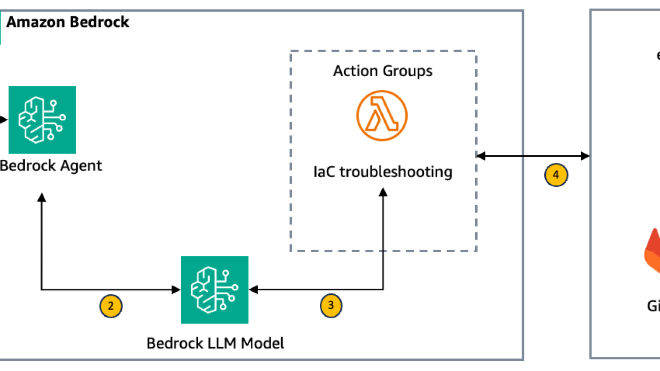
Accelerate IaC troubleshooting with Amazon Bedrock Agents
Troubleshooting infrastructure as code (IaC) errors often consumes valuable time and resources. Developers can spend multiple cycles searching for solutions across forums, troubleshooting repetitive issues, or trying to identify the root cause. These delays can lead to missed security errors or compliance violations, especially in complex, multi-account environments.
This post demonstrates how you can use Amazon Bedrock Agents to create an intelligent solution to streamline the resolution of Terraform and AWS CloudFormation code issues through context-aware troubleshooting. Amazon Bedrock is a fully managed service that offers a choice of high-performing foundation models (FMs) from leading AI companies like AI21 Labs, Anthropic, Cohere, Meta, Stability AI, and Amazon through a single API, along with a broad set of capabilities to build generative AI applications with security, privacy, and responsible AI. Amazon Bedrock Agents is a fully managed service that helps developers create AI agents that can break down complex tasks into steps and execute them using FMs and APIs to accomplish specific business objectives.
Our solution uses Amazon Bedrock Agents to analyze error messages and code context, generating detailed troubleshooting steps for IaC errors. In organizations with multi-account AWS environments, teams often maintain a centralized AWS environment for developers to deploy applications. This setup makes sure that AWS infrastructure deployments using IaC align with organizational security and compliance measures. For specific IaC errors related to these compliance measures, such as those involving service control policies (SCPs) or resource-based policies, our solution intelligently directs developers to contact appropriate teams like Security or Enablement. This targeted guidance maintains security protocols and makes sure that sensitive issues are handled by the right experts. The solution is flexible and can be adapted for similar use cases beyond these examples.
Although we focus on Terraform Cloud workspaces in this example, the same principles apply to GitLab CI/CD pipelines or other continuous integration and delivery (CI/CD) approaches executing IaC code. By automating initial error analysis and providing targeted solutions or guidance, you can improve operational efficiency and focus on solving complex infrastructure challenges within your organization’s compliance framework.
Solution overview
Before we dive into the deployment process, let’s walk through the key steps of the architecture as illustrated in the following figure.

The workflow for the Terraform solution is as follows:
- Initial input through the Amazon Bedrock Agents chat console – The user begins by entering details about their Terraform error into the chat console for Amazon Bedrock Agents. This typically includes the Terraform Cloud workspace URL where the error occurred, and optionally, a Git repository URL and branch name if additional context is needed.
- Error retrieval and context gathering – The Amazon Bedrock agent forwards these details to an action group that invokes the first AWS Lambda function (see the following Lambda function code). This function invokes another Lambda function (see the following Lambda function code) which retrieves the latest error message from the specified Terraform Cloud workspace. If a Git repository URL is provided, it also retrieves relevant Terraform files from the repository. This contextual information is then sent back to the first Lambda function.
- Error analysis and response generation – Lambda function would then construct a detailed prompt that includes the error message, repository files (if available), and specific use case instructions. It then uses the Amazon Bedrock model to analyze the error and generate either troubleshooting steps or guidance to contact specific teams.
- Interaction and user guidance – The agent displays the generated response to the user. For most Terraform errors, this includes detailed troubleshooting steps. For specific cases related to organizational policies (for example, service control policies or resource-based policies), the response directs the user to contact the appropriate team, such as Security or Enablement.
- Continuous improvement – The solution can be continually updated with new specific use cases and organizational guidelines, making sure that the troubleshooting advice stays current with the organization’s evolving infrastructure and compliance requirements. For example:
- SCP or IAM policy violations – Guides developers when they encounter permission issues due to SCPs or strict AWS Identity and Access Management (IAM) boundaries, offering alternatives or escalation paths.
- VPC and networking restrictions – Flags non-compliant virtual private cloud (VPC) or subnet configurations (such as public subnets) and suggests security-compliant adjustments.
- Encryption requirements – Detects missing or incorrect encryption for Amazon Simple Storage Service (Amazon S3) or Amazon Elastic Block Store (Amazon EBS) resources and recommends the appropriate configurations to align with compliance standards.
The following diagram illustrates the step-by-step process of how the solution works.

This solution streamlines the process of resolving Terraform errors, providing immediate, context-aware guidance to developers while making sure that sensitive or complex issues are directed to the appropriate teams. By using the capabilities of Amazon Bedrock Agents, it offers a scalable and intelligent approach to managing IaC challenges in large, multi-account AWS environments.
Prerequisites
To implement the solution, you need the following:
- An understanding of Amazon Bedrock Agents, prompt engineering, Amazon Bedrock Knowledge Bases, Lambda functions, and IAM
- An AWS account with appropriate IAM permissions to create agents and knowledge bases in Amazon Bedrock, Lambda functions, and IAM roles
- A service role created for Amazon Bedrock Agents
- Model access enabled for Amazon Bedrock
- A GitLab account with a repository and a personal access token to access the repository
Create the Amazon Bedrock agent
To create and configure the Amazon Bedrock agent, complete the following steps:
- On the Amazon Bedrock console, choose Agents in the navigation pane.
- Choose Create agent.
- Provide agent details, including agent name and description (optional).
- Grant the agent permissions to AWS services through the IAM service role. This gives your agent access to required services, such as Lambda.
- Select an FM from Amazon Bedrock (such as Anthropic’s Claude 3 Sonnet).
- For troubleshooting Terraform errors through Amazon Bedrock Agents, attach the following instruction to the agent. This instruction makes sure that the agent gathers the required input from the user and executes the action group to provide detailed troubleshooting steps.
“You are a terraform code error specialist. Greet the user and ask for terraform workspace url, branch name, code repository url. Once received, trigger troubleshooting action group. Provide the troubleshooting steps to the user.”
Configure the Lambda function for the action group
After you configure the initial agent and add the preceding instruction to the agent, you need to create two Lambda functions:
- The first Lambda function will be added to the action group, which is invoked by the Amazon Bedrock agent, and will subsequently trigger the second Lambda function using the invoke method. Refer to the Lambda function code for more details. Make sure the LAMBDA_2_FUNCTION_NAME environment variable is set.
- The second Lambda function will handle fetching the Terraform workspace error and the associated Terraform code from GitLab. Refer to the Lambda function code. Make sure that the TERRAFORM_API_URL, TERRAFORM_SECRET_NAME, and VCS_SECRET_NAME environment variables are set.
After the Terraform workspace error and code details are retrieved, these details will be passed back to the first Lambda function, which will use the Amazon Bedrock API with an FM to generate and provide the appropriate troubleshooting steps based on the error and code information.
Add the action group to the Amazon Bedrock agent
Complete the following steps to add the action group to the Amazon Bedrock agent:
- Add an action group to the Amazon Bedrock agent.
- Assign a descriptive name (for example, troubleshooting) to the action group and provide a description. This helps clarify the purpose of the action group within the workflow.
- For Action group type, select Define with function details.
For more details, see Define function details for your agent’s action groups in Amazon Bedrock.
- For Action group invocation, choose the first Lambda function that you created previously.
This function runs the business logic required when an action is invoked. Make sure to choose the correct version of the first Lambda function. For more details on how to configure Lambda functions for action groups, see Configure Lambda functions to send information that an Amazon Bedrock agent elicits from the user.
- For Action group function 1, provide a name and description.
- Add the following parameters.
|
Name |
Description | Type | Required |
| workspace_url |
Terraform workspace url |
string |
True |
| repo_url |
Code repository URL |
string |
True |
| branch_name | Code repository branch name | string |
True |
Test the solution
The following example is of a Terraform error due to a service control polcy. The troubleshooting steps provided would be aligned to address those specific constraints. The action group triggers the Lambda function, which follows structured single-shot prompting by passing the complete context—such as the error message and repository contents—in a single input to the Amazon Bedrock model to generate precise troubleshooting steps.
Example 1: The following screenshot shows an example of a Terraform error caused by an SCP limitation managed by the security team.

The following screenshot shows an example of the user interaction with Amazon Bedrock Agents and the troubleshooting steps provided.

Example 2: The following screenshot shows an example of a Terraform error due to a missing variable value.

The following screenshot shows an example of the user interaction with Amazon Bedrock Agents and the troubleshooting steps provided.

Clean up
The services used in this demo can incur costs. Complete the following steps to clean up your resources:
- Delete the Lambda functions if they are no longer required.
- Delete the action group and Amazon Bedrock agent you created.
Conclusion
IaC offers flexibility for managing cloud environments, but troubleshooting code errors can be time-consuming, especially in environments with strict organizational guardrails. This post demonstrated how Amazon Bedrock Agents, combined with action groups and generative AI models, streamlines and accelerates the resolution of Terraform errors while maintaining compliance with environment security and operational guidelines.
Using the capabilities of Amazon Bedrock Agents, developers can receive context-aware troubleshooting steps tailored to environment-related issues such as SCP or IAM violations, VPC restrictions, and encryption policies. The solution provides specific guidance based on the error’s context and directs users to the appropriate teams for issues that require further escalation. This reduces the time spent on IaC errors, improves developer productivity, and maintains organizational compliance.
Are you ready to streamline your cloud deployment process with the generative AI of Amazon Bedrock? Start by exploring the Amazon Bedrock User Guide to see how it can facilitate your organization’s transition to the cloud. For specialized assistance, consider engaging with AWS Professional Services to maximize the efficiency and benefits of using Amazon Bedrock.
About the Authors
 Akhil Raj Yallamelli is a Cloud Infrastructure Architect at AWS, specializing in architecting cloud infrastructure solutions for enhanced data security and cost efficiency. He is experienced in integrating technical solutions with business strategies to create scalable, reliable, and secure cloud environments. Akhil enjoys developing solutions focusing on customer business outcomes, incorporating generative AI (Gen AI) technologies to drive innovation and cloud enablement. He holds an MS degree in Computer Science. Outside of his professional work, Akhil enjoys watching and playing sports.
 Ebbey Thomas is a Senior Generative AI Specialist Solutions Architect at AWS. He designs and implements generative AI solutions that address specific customer business problems. He is recognized for simplifying complexity and delivering measurable business outcomes for clients. Ebbey holds a BS in Computer Engineering and an MS in Information Systems from Syracuse University.