Posts in category: Amazon AWS

A common use case with generative AI that we usually see customers evaluate for a production use case is a generative AI-powered assistant. However, before it can be deployed, there is the typical production readiness assessment that includes concerns such as understanding the security posture, monitoring and logging, cost tracking, resilience, and more. The highest priority of these production readiness assessments is usually security. If there are security risks that can’t be clearly identified, then they can’t be addressed, and that can halt the production deployment of the generative AI application.

In this post, we show you an example of a generative AI assistant application and demonstrate how to assess its security posture using the OWASP Top 10 for Large Language Model Applications, as well as how to apply mitigations for common threats.

Generative AI scoping framework

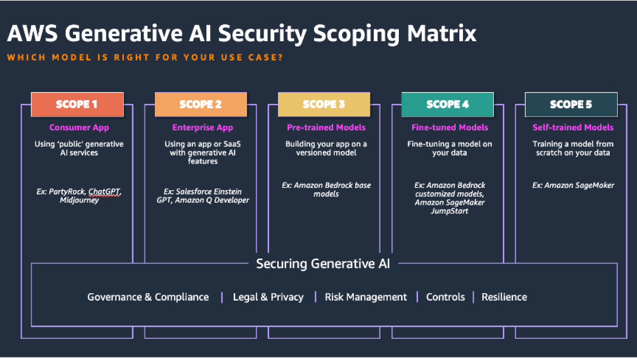
Start by understanding where your generative AI application fits within the spectrum of managed vs. custom. Use the AWS generative AI scoping framework to understand the specific mix of the shared responsibility for the security controls applicable to your application. For example, Scope 1 “Consumer Apps” like PartyRock or ChatGPT are usually publicly facing applications, where most of the application internal security is owned and controlled by the provider, and your responsibility for security is on the consumption side. Contrast that with Scope 4/5 applications, where not only do you build and secure the generative AI application yourself, but you are also responsible for fine-tuning and training the underlying large language model (LLM). The security controls in scope for Scope 4/5 applications will range more broadly from the frontend to LLM model security. This post will focus on the Scope 3 generative AI assistant application, which is one of the more frequent use cases seen in the field.

The following figure of the AWS Generative AI Security Scoping Matrix summarizes the types of models for each scope.

OWASP Top 10 for LLMs

Using the OWASP Top 10 for understanding threats and mitigations to an application is one of the most common ways application security is assessed. The OWASP Top 10 for LLMs takes a tried and tested framework and applies it to generative AI applications to help us discover, understand, and mitigate the novel threats for generative AI.

Solution overview

Let’s start with a logical architecture of a typical generative AI assistant application overlying the OWASP Top 10 for LLM threats, as illustrated in the following diagram.

In this architecture, the end-user request usually goes through the following components:

• Authentication layer – This layer validates that the user connecting to the application is who they say they are. This is typically done through some sort of an identity provider (IdP) capability like Okta, AWS IAM Identity Center, or Amazon Cognito.
• Application controller – This layer contains most of the application business logic and determines how to process the incoming user request by generating the LLM prompts and processing LLM responses before they are sent back to the user.
• LLM and LLM agent – The LLM provides the core generative AI capability to the assistant. The LLM agent is an orchestrator of a set of steps that might be necessary to complete the desired request. These steps might involve both the use of an LLM and external data sources and APIs.
• Agent plugin controller – This component is responsible for the API integration to external data sources and APIs. This component also holds the mapping between the logical name of an external component, which the LLM agent might refer to, and the physical name.
• RAG data store – The Retrieval Augmented Generation (RAG) data store delivers up-to-date, precise, and access-controlled knowledge from various data sources such as data warehouses, databases, and other software as a service (SaaS) applications through data connectors.

The OWASP Top 10 for LLM risks map to various layers of the application stack, highlighting vulnerabilities from UIs to backend systems. In the following sections, we discuss risks at each layer and provide an application design pattern for a generative AI assistant application in AWS that mitigates these risks.

The following diagram illustrates the assistant architecture on AWS.

Authentication layer (Amazon Cognito)

Common security threats such as brute force attacks, session hijacking, and denial of service (DoS) attacks can occur. To mitigate these risks, implement best practices like multi-factor authentication (MFA), rate limiting, secure session management, automatic session timeouts, and regular token rotation. Additionally, deploying edge security measures such as AWS WAF and distributed denial of service (DDoS) mitigation helps block common web exploits and maintain service availability during attacks.

In the preceding architecture diagram, AWS WAF is integrated with Amazon API Gateway to filter incoming traffic, blocking unintended requests and protecting applications from threats like SQL injection, cross-site scripting (XSS), and DoS attacks. AWS WAF Bot Control further enhances security by providing visibility and control over bot traffic, allowing administrators to block or rate-limit unwanted bots. This feature can be centrally managed across multiple accounts using AWS Firewall Manager, providing a consistent and robust approach to application protection.

Amazon Cognito complements these defenses by enabling user authentication and data synchronization. It supports both user pools and identity pools, enabling seamless management of user identities across devices and integration with third-party identity providers. Amazon Cognito offers security features, including MFA, OAuth 2.0, OpenID Connect, secure session management, and risk-based adaptive authentication, to help protect against unauthorized access by evaluating sign-in requests for suspicious activity and responding with additional security measures like MFA or blocking sign-ins. Amazon Cognito also enforces password reuse prevention, further protecting against compromised credentials.

AWS Shield Advanced adds an extra layer of defense by providing enhanced protection against sophisticated DDoS attacks. Integrated with AWS WAF, Shield Advanced delivers comprehensive perimeter protection, using tailored detection and health-based assessments to enhance response to attacks. It also offers round-the-clock support from the AWS Shield Response Team and includes DDoS cost protection, making applications remain secure and cost-effective. Together, Shield Advanced and AWS WAF create a security framework that protects applications against a wide range of threats while maintaining availability.

This comprehensive security setup addresses LLM10:2025 Unbound Consumption and LLM02:2025 Sensitive Information Disclosure, making sure that applications remain both resilient and secure.

Application controller layer (LLM orchestrator Lambda function)

The application controller layer is usually vulnerable to risks such as LLM01:2025 Prompt Injection, LLM05:2025 Improper Output Handling, and LLM 02:2025 Sensitive Information Disclosure. Outside parties might frequently attempt to exploit this layer by crafting unintended inputs to manipulate the LLM, potentially causing it to reveal sensitive information or compromise downstream systems.

In the physical architecture diagram, the application controller is the LLM orchestrator AWS Lambda function. It performs strict input validation by extracting the event payload from API Gateway and conducting both syntactic and semantic validation. By sanitizing inputs, applying allowlisting and deny listing of keywords, and validating inputs against predefined formats or patterns, the Lambda function helps prevent LLM01:2025 Prompt Injection attacks. Additionally, by passing the user_id downstream, it enables the downstream application components to mitigate the risk of sensitive information disclosure, addressing concerns related to LLM02:2025 Sensitive Information Disclosure.

Amazon Bedrock Guardrails provides an additional layer of protection by filtering and blocking sensitive content, such as personally identifiable information (PII) and other custom sensitive data defined by regex patterns. Guardrails can also be configured to detect and block offensive language, competitor names, or other undesirable terms, making sure that both inputs and outputs are safe. You can also use guardrails to prevent LLM01:2025 Prompt Injection attacks by detecting and filtering out harmful or manipulative prompts before they reach the LLM, thereby maintaining the integrity of the prompt.

Another critical aspect of security is managing LLM outputs. Because the LLM might generate content that includes executable code, such as JavaScript or Markdown, there is a risk of XSS attacks if this content is not properly handled. To mitigate this risk, apply output encoding techniques, such as HTML entity encoding or JavaScript escaping, to neutralize any potentially harmful content before it is presented to users. This approach addresses the risk of LLM05:2025 Improper Output Handling.

Implementing Amazon Bedrock prompt management and versioning allows for continuous improvement of the user experience while maintaining the overall security of the application. By carefully managing changes to prompts and their handling, you can enhance functionality without introducing new vulnerabilities and mitigating LLM01:2025 Prompt Injection attacks.

Treating the LLM as an untrusted user and applying human-in-the-loop processes over certain actions are strategies to lower the likelihood of unauthorized or unintended operations.

LLM and LLM agent layer (Amazon Bedrock LLMs)

The LLM and LLM agent layer frequently handles interactions with the LLM and faces risks such as LLM10: Unbounded Consumption, LLM05:2025 Improper Output Handling, and LLM02:2025 Sensitive Information Disclosure.

DoS attacks can overwhelm the LLM with multiple resource-intensive requests, degrading overall service quality while increasing costs. When interacting with Amazon Bedrock hosted LLMs, setting request parameters such as the maximum length of the input request will minimize the risk of LLM resource exhaustion. Additionally, there is a hard limit on the maximum number of queued actions and total actions an Amazon Bedrock agent can take to fulfill a customer’s intent, which limits the number of actions in a system reacting to LLM responses, avoiding unnecessary loops or intensive tasks that could exhaust the LLM’s resources.

Improper output handling leads to vulnerabilities such as remote code execution, cross-site scripting, server-side request forgery (SSRF), and privilege escalation. The inadequate validation and management of the LLM-generated outputs before they are sent downstream can grant indirect access to additional functionality, effectively enabling these vulnerabilities. To mitigate this risk, treat the model as any other user and apply validation of the LLM-generated responses. The process is facilitated with Amazon Bedrock Guardrails using filters such as content filters with configurable thresholds to filter harmful content and safeguard against prompt attacks before they are processed further downstream by other backend systems. Guardrails automatically evaluate both user input and model responses to detect and help prevent content that falls into restricted categories.

Amazon Bedrock Agents execute multi-step tasks and securely integrate with AWS native and third-party services to reduce the risk of insecure output handling, excessive agency, and sensitive information disclosure. In the architecture diagram, the action group Lambda function under the agents is used to encode all the output text, making it automatically non-executable by JavaScript or Markdown. Additionally, the action group Lambda function parses each output from the LLM at every step executed by the agents and controls the processing of the outputs accordingly, making sure they are safe before further processing.

Sensitive information disclosure is a risk with LLMs because malicious prompt engineering can cause LLMs to accidentally reveal unintended details in their responses. This can lead to privacy and confidentiality violations. To mitigate the issue, implement data sanitization practices through content filters in Amazon Bedrock Guardrails.

Additionally, implement custom data filtering policies based on user_id and strict user access policies. Amazon Bedrock Guardrails helps filter content deemed sensitive, and Amazon Bedrock Agents further reduces the risk of sensitive information disclosure by allowing you to implement custom logic in the preprocessing and postprocessing templates to strip any unexpected information. If you have enabled model invocation logging for the LLM or implemented custom logging logic in your application to record the input and output of the LLM in Amazon CloudWatch, measures such as CloudWatch Log data protection are important in masking sensitive information identified in the CloudWatch logs, further mitigating the risk of sensitive information disclosure.

Agent plugin controller layer (action group Lambda function)

The agent plugin controller frequently integrates with internal and external services and applies custom authorization to internal and external data sources and third-party APIs. At this layer, the risk of LLM08:2025 Vector & Embedding Weaknesses and LLM06:2025 Excessive Agency are in effect. Untrusted or unverified third-party plugins could introduce backdoors or vulnerabilities in the form of unexpected code.

Apply least privilege access to the AWS Identity and Access Management (IAM) roles of the action group Lambda function, which interacts with plugin integrations to external systems to help mitigate the risk of LLM06:2025 Excessive Agency and LLM08:2025 Vector & Embedding Weaknesses. This is demonstrated in the physical architecture diagram; the agent plugin layer Lambda function is associated with a least privilege IAM role for secure access and interface with other internal AWS services.

Additionally, after the user identity is determined, restrict the data plane by applying user-level access control by passing the user_id to downstream layers like the agent plugin layer. Although this user_id parameter can be used in the agent plugin controller Lambda function for custom authorization logic, its primary purpose is to enable fine-grained access control for third-party plugins. The responsibility lies with the application owner to implement custom authorization logic within the action group Lambda function, where the user_id parameter can be used in combination with predefined rules to apply the appropriate level of access to third-party APIs and plugins. This approach wraps deterministic access controls around a non-deterministic LLM and enables granular access control over which users can access and execute specific third-party plugins.

Combining user_id-based authorization on data and IAM roles with least privilege on the action group Lambda function will generally minimize the risk of LLM08:2025 Vector & Embedding Weaknesses and LLM06:2025 Excessive Agency.

RAG data store layer

The RAG data store is responsible for securely retrieving up-to-date, precise, and user access-controlled knowledge from various first-party and third-party data sources. By default, Amazon Bedrock encrypts all knowledge base-related data using an AWS managed key. Alternatively, you can choose to use a customer managed key. When setting up a data ingestion job for your knowledge base, you can also encrypt the job using a custom AWS Key Management Service (AWS KMS) key.

If you decide to use the vector store in Amazon OpenSearch Service for your knowledge base, Amazon Bedrock can pass a KMS key of your choice to it for encryption. Additionally, you can encrypt the sessions in which you generate responses from querying a knowledge base with a KMS key. To facilitate secure communication, Amazon Bedrock Knowledge Bases uses TLS encryption when interacting with third-party vector stores, provided that the service supports and permits TLS encryption in transit.

Regarding user access control, Amazon Bedrock Knowledge Bases uses filters to manage permissions. You can build a segmented access solution on top of a knowledge base using metadata and filtering feature. During runtime, your application must authenticate and authorize the user, and include this user information in the query to maintain accurate access controls. To keep the access controls updated, you should periodically resync the data to reflect any changes in permissions. Additionally, groups can be stored as a filterable attribute, further refining access control.

This approach helps mitigate the risk of LLM02:2025 Sensitive Information Disclosure and LLM08:2025 Vector & Embedding Weaknesses, to assist in that only authorized users can access the relevant data.

Summary

In this post, we discussed how to classify your generative AI application from a security shared responsibility perspective using the AWS Generative AI Security Scoping Matrix. We reviewed a common generative AI assistant application architecture and assessed its security posture using the OWASP Top 10 for LLMs framework, and showed how to apply the OWASP Top 10 for LLMs threat mitigations using AWS service controls and services to strengthen the architecture of your generative AI assistant application. Learn more about building generative AI applications with AWS Workshops for Bedrock.

About the Authors

Syed Jaffry is a Principal Solutions Architect with AWS. He advises software companies on AI and helps them build modern, robust and secure application architectures on AWS.

Amit Kumar Agrawal is a Senior Solutions Architect at AWS where he has spent over 5 years working with large ISV customers. He helps organizations build and operate cost-efficient and scalable solutions in the cloud, driving their business and technical outcomes.

Tej Nagabhatla is a Senior Solutions Architect at AWS, where he works with a diverse portfolio of clients ranging from ISVs to large enterprises. He specializes in providing architectural guidance across a wide range of topics around AI/ML, security, storage, containers, and serverless technologies. He helps organizations build and operate cost-efficient, scalable cloud applications. In his free time, Tej enjoys music, playing basketball, and traveling.

Read More

Attaching a custom Docker image to an Amazon SageMaker Studio domain involves several steps. First, you need to build and push the image to Amazon Elastic Container Registry (Amazon ECR). You also need to make sure that the Amazon SageMaker domain execution role has the necessary permissions to pull the image from Amazon ECR. After the image is pushed to Amazon ECR, you create a SageMaker custom image on the AWS Management Console. Lastly, you update the SageMaker domain configuration to specify the custom image Amazon Resource Name (ARN). This multi-step process needs to be followed manually every time end-users create new custom Docker images to make them available in SageMaker Studio.

In this post, we explain how to automate this process. This approach allows you to update the SageMaker configuration without writing additional infrastructure code, provision custom images, and attach them to SageMaker domains. By adopting this automation, you can deploy consistent and standardized analytics environments across your organization, leading to increased team productivity and mitigating security risks associated with using one-time images.

The solution described in this post is geared towards machine learning (ML) engineers and platform teams who are often responsible for managing and standardizing custom environments at scale across an organization. For individual data scientists seeking a self-service experience, we recommend that you use the native Docker support in SageMaker Studio, as described in Accelerate ML workflows with Amazon SageMaker Studio Local Mode and Docker support. This feature allows data scientists to build, test, and deploy custom Docker containers directly within the SageMaker Studio integrated development environment (IDE), enabling you to iteratively experiment with your analytics environments seamlessly within the familiar SageMaker Studio interface.

Solution overview

The following diagram illustrates the solution architecture.

We deploy a pipeline using AWS CodePipeline, which automates a custom Docker image creation and attachment of the image to a SageMaker domain. The pipeline first checks out the code base from the GitHub repo and creates custom Docker images based on the configuration declared in the config files. After successfully creating and pushing Docker images to Amazon ECR, the pipeline validates the image by scanning and checking for security vulnerabilities in the image. If no critical or high-security vulnerabilities are found, the pipeline continues to the manual approval stage before deployment. After manual approval is complete, the pipeline deploys the SageMaker domain and attaches custom images to the domain automatically.

Prerequisites

The prerequisites for implementing the solution described in this post include:

• An AWS account and access to the account and access to deploy AWS CloudFormation templates
• js and the npm command line interface
• The AWS Cloud Development Kit (AWS CDK) installed
• Version 2 of the AWS Command Line Interface (AWS CLI) installed
• The Git command line interface installed on your computer for cloning the repository
• The complete AWS CDK bootstrapping in your AWS account

Deploy the solution

Complete the following steps to implement the solution:

1. Log in to your AWS account using the AWS CLI in a shell terminal (for more details, see Authenticating with short-term credentials for the AWS CLI).
2. Run the following command to make sure you have successfully logged in to your AWS account:

aws sts get-caller-identity

4. Fork the the GitHub repo to your GitHub account .
5. Clone the forked repo to your local workstation using the following command:

git clone <clone_url_of_forked_repo>

6. Log in to the console and create an AWS CodeStar connection to the GitHub repo in the previous step. For instructions, see Create a connection to GitHub (console).
7. Copy the ARN for the connection you created.
8. Go to the terminal and run the following command to cd into the repository directory:

cd streamline-sagemaker-custom-images-cicd

9. Run the following command to install all libraries from npm:

npm install

10. Run the following commands to run a shell script in the terminal. This script will take your AWS account number and AWS Region as input parameters and deploy an AWS CDK stack, which deploys components such as CodePipeline, AWS CodeBuild, the ECR repository, and so on. Use an existing VPC to setup VPC_ID export variable below. If you don’t have a VPC, create one with at least two subnets and use it.

export AWS_ACCOUNT=$(aws sts get-caller-identity --query Account --output text)
export AWS_REGION=<YOUR_AWS_REGION>
export VPC_ID=<VPC_ID_TO_DEPLOY>
export CODESTAR_CONNECTION_ARN=<CODE_STAR_CONNECTION_ARN_CREATED_IN_ABOVE_STEP>
export REPOSITORY_OWNER=<YOUR_GITHUB_LOGIN_ID>

11. Run the following command to deploy the AWS infrastructure using the AWS CDK V2 and make sure to wait for the template to succeed:

cdk deploy PipelineStack --require-approval never

12. On the CodePipeline console, choose Pipelines in the navigation pane.
13. Choose the link for the pipeline named sagemaker-custom-image-pipeline.

14. You can follow the progress of the pipeline on the console and provide approval in the manual approval stage to deploy the SageMaker infrastructure. Pipeline takes approximately 5-8 min to build image and move to manual approval stage
15. Wait for the pipeline to complete the deployment stage.

The pipeline creates infrastructure resources in your AWS account with a SageMaker domain and a SageMaker custom image. It also attaches the custom image to the SageMaker domain.

16. On the SageMaker console, choose Domains under Admin configurations in the navigation pane.

17. Open the domain named team-ds, and navigate to the Environment

You should be able to see one custom image that is attached.

How custom images are deployed and attached

CodePipeline has a stage called BuildCustomImages that contains the automated steps to create a SageMaker custom image using the SageMaker Custom Image CLI and push it to the ECR repository created in the AWS account. The AWS CDK stack at the deployment stage has the required steps to create a SageMaker domain and attach a custom image to the domain. The parameters to create the SageMaker domain, custom image, and so on are configured in JSON format and used in the SageMaker stack under the lib directory. Refer to the sagemakerConfig section in environments/config.json for declarative parameters.

Add more custom images

Now you can add your own custom Docker image to attach to the SageMaker domain created by the pipeline. For the custom images being created, refer to Dockerfile specifications for the Docker image specifications.

1. cd into the images directory in the repository in the terminal:

cd images

2. Create a new directory (for example, custom) under the images directory:

mkdir custom

3. Add your own Dockerfile to this directory. For testing, you can use the following Dockerfile config:

FROM public.ecr.aws/amazonlinux/amazonlinux:2
ARG NB_USER="sagemaker-user"
ARG NB_UID="1000"
ARG NB_GID="100"
RUN yum update -y && 
    yum install python3 python3-pip shadow-utils -y && 
    yum clean all
RUN yum install --assumeyes python3 shadow-utils && 
    useradd --create-home --shell /bin/bash --gid "${NB_GID}" --uid ${NB_UID} ${NB_USER} && 
    yum clean all && 
    python3 -m pip install jupyterlab
RUN python3 -m pip install --upgrade pip
RUN python3 -m pip install --upgrade urllib3==1.26.6
USER ${NB_UID}
CMD jupyter lab --ip 0.0.0.0 --port 8888 
--ServerApp.base_url="/jupyterlab/default" 
--ServerApp.token='' 
--ServerApp.allow_origin='*'

4. Update the images section in the json file under the environments directory to add the new image directory name you have created:

"images": [
      "repositoryName": "research-platform-ecr",
       "tags":[
         "jlab",
         "custom" << Add here
       ]
      }
    ]

5. Update the same image name in customImages under the created SageMaker domain configuration:

"customImages":[
          "jlab",
          "custom" << Add here
 ],

6. Commit and push changes to the GitHub repository.
7. You should see CodePipeline is triggered upon push. Follow the progress of the pipeline and provide manual approval for deployment.

After deployment is completed successfully, you should be able to see that the custom image you have added is attached to the domain configuration (as shown in the following screenshot).

Clean up

To clean up your resources, open the AWS CloudFormation console and delete the stacks SagemakerImageStack and PipelineStack in that order. If you encounter errors such as “S3 Bucket is not empty” or “ECR Repository has images,” you can manually delete the S3 bucket and ECR repository that was created. Then you can retry deleting the CloudFormation stacks.

Conclusion

In this post, we showed how to create an automated continuous integration and delivery (CI/CD) pipeline solution to build, scan, and deploy custom Docker images to SageMaker Studio domains. You can use this solution to promote consistency of the analytical environments for data science teams across your enterprise. This approach helps you achieve machine learning (ML) governance, scalability, and standardization.

About the Authors

Muni Annachi, a Senior DevOps Consultant at AWS, boasts over a decade of expertise in architecting and implementing software systems and cloud platforms. He specializes in guiding non-profit organizations to adopt DevOps CI/CD architectures, adhering to AWS best practices and the AWS Well-Architected Framework. Beyond his professional endeavors, Muni is an avid sports enthusiast and tries his luck in the kitchen.

Ajay Raghunathan is a Machine Learning Engineer at AWS. His current work focuses on architecting and implementing ML solutions at scale. He is a technology enthusiast and a builder with a core area of interest in AI/ML, data analytics, serverless, and DevOps. Outside of work, he enjoys spending time with family, traveling, and playing football.

Arun Dyasani is a Senior Cloud Application Architect at AWS. His current work focuses on designing and implementing innovative software solutions. His role centers on crafting robust architectures for complex applications, leveraging his deep knowledge and experience in developing large-scale systems.

Shweta Singh is a Senior Product Manager in the Amazon SageMaker Machine Learning platform team at AWS, leading the SageMaker Python SDK. She has worked in several product roles in Amazon for over 5 years. She has a Bachelor of Science degree in Computer Engineering and a Masters of Science in Financial Engineering, both from New York University.

Jenna Eun is a Principal Practice Manager for the Health and Advanced Compute team at AWS Professional Services. Her team focuses on designing and delivering data, ML, and advanced computing solutions for the public sector, including federal, state and local governments, academic medical centers, nonprofit healthcare organizations, and research institutions.

Meenakshi Ponn Shankaran is a Principal Domain Architect at AWS in the Data & ML Professional Services Org. He has extensive expertise in designing and building large-scale data lakes, handling petabytes of data. Currently, he focuses on delivering technical leadership to AWS US Public Sector clients, guiding them in using innovative AWS services to meet their strategic objectives and unlock the full potential of their data.

Read More

The rise of AI has opened new avenues for enhancing customer experiences across multiple channels. Technologies like natural language understanding (NLU) are employed to discern customer intents, facilitating efficient self-service actions. Automatic speech recognition (ASR) translates spoken words into text, enabling seamless voice interactions. With Amazon Lex bots, businesses can use conversational AI to integrate these capabilities into their call centers. Amazon Lex uses ASR and NLU to comprehend customer needs, guiding them through their journey. These AI technologies have significantly reduced agent handle times, increased Net Promoter Scores (NPS), and streamlined self-service tasks, such as appointment scheduling.

The advent of generative AI further expands the potential to enhance omnichannel customer experiences. However, concerns about security, compliance, and AI hallucinations often deter businesses from directly exposing customers to large language models (LLMs) through their omnichannel solutions. This is where the integration of Amazon Lex and Amazon Bedrock becomes invaluable. In this setup, Amazon Lex serves as the initial touchpoint, managing intent classification, slot collection, and fulfillment. Meanwhile, Amazon Bedrock acts as a secondary validation layer, intervening when Amazon Lex encounters uncertainties in understanding customer inputs.

In this post, we demonstrate how to integrate LLMs into your omnichannel experience using Amazon Lex and Amazon Bedrock.

Enhancing customer interactions with LLMs

The following are three scenarios illustrating how LLMs can enhance customer interactions:

• Intent classification – These scenarios occur when a customer clearly articulates their intent, but the lack of utterance training data results in poor performance by traditional models. For example, a customer might call in and say, “My basement is flooded, there is at least a foot of water, and I have no idea what to do.” Traditional NLU models might lack the training data to handle this out-of-band response, because they’re typically trained on sample utterances like “I need to make a claim,” “I have a flood claim,” or “Open claim,” which are mapped to a hypothetical StartClaim intent. However, an LLM, when provided with the context of each intent including a description and sample utterances, can accurately determine that the customer is dealing with a flooded basement and is seeking to start a claim.
• Assisted slot resolution (built-in) and custom slot assistance (custom) – These scenarios occur when a customer says an out-of-band response to a slot collection. For select built-in slot types such as AMAZON.Date, AMAZON.Country, and AMAZON.Confirmation, Amazon Lex currently has a built-in capability to handle slot resolution for select built-in slot types. For custom slot types, you would need to implement custom logic using AWS Lambda for slot resolution and additional validation. This solution handles custom slot resolution by using LLMs to clarify and map these inputs to the correct slots. For example, interpreting “Toyota Tundra” as “truck” or “the whole dang top of my house is gone” as “roof.” This allows you to integrate generative AI to validate both your pre-built slots and your custom slots.
• Background noise mitigation – Many customers can’t control the background noise when calling into a call center. This noise might include a loud TV, a sidebar conversation, or non-human sounds being transcribed as voice (for example, a car passing by and is transcribed as “uhhh”). In such cases, the NLU model, depending on its training data, might misclassify the caller’s intent or require the caller to repeat themselves. However, with an LLM, you can provide the transcript with appropriate context to distinguish the noise from the customer’s actual statement. For example, if a TV show is playing in the background and the customer says “my car” when asked about their policy, the transcription might read “Tune in this evening for my car.” The LLM can ignore the irrelevant portion of the transcription and focus on the relevant part, “my car,” to accurately understand the customer’s intent.

As demonstrated in these scenarios, the LLM is not controlling the conversation. Instead, it operates within the boundaries defined by intents, intent descriptions, slots, sample slots, and utterances from Amazon Lex. This approach helps guide the customer along the correct path, reducing the risks of hallucination and manipulation of the customer-facing application. Furthermore, this approach reduces cost, because NLU is used when possible, and the LLM acts as a secondary check before re-prompting the customer.

You can further enhance this AI-driven experience by integrating it with your contact center solution, such as Amazon Connect. By combining the capabilities of Amazon Lex, Amazon Bedrock, and Amazon Connect, you can deliver a seamless and intelligent customer experience across your channels.

When customers reach out, whether through voice or chat, this integrated solution provides a powerful, AI-driven interaction:

1. Amazon Connect manages the initial customer contact, handling call routing and channel selection.
2. Amazon Lex processes the customer’s input, using NLU to identify intent and extract relevant information.
3. In cases where Amazon Lex might not fully understand the customer’s intent or when a more nuanced interpretation is needed, advanced language models in Amazon Bedrock can be invoked to provide deeper analysis and understanding.
4. The combined insights from Amazon Lex and Amazon Bedrock guide the conversation flow in Amazon Connect, determining whether to provide automated responses, request more information, or route the customer to a human agent.

Solution overview

In this solution, Amazon Lex will connect to Amazon Bedrock through Lambda, and invoke an LLM of your choice on Amazon Bedrock when assistance in intent classification and slot resolution is needed throughout the conversation. For instance, if an ElicitIntent call defaults to the FallbackIntent, the Lambda function runs to have Amazon Bedrock determine if the user potentially used out-of-band phrases that should be properly mapped. Additionally, we can augment the prompts sent to the model for intent classification and slot resolution with business context to yield more accurate results. Example prompts for intent classification and slot resolution is available in the GitHub repo.

The following diagram illustrates the solution architecture:

The workflow consists of the following steps:

1. Messages are sent to the Amazon Lex omnichannel using Amazon Connect (text and voice), messaging apps (text), and third-party contact centers (text and voice). Amazon Lex NLU maps user utterances to specific intents.
2. The Lambda function is invoked at certain phases of the conversation where Amazon Lex NLU didn’t identify the user utterance, such as during the fallback intent or during slot fulfillment.
3. Lambda calls foundation models (FMs) selected from an AWS CloudFormation template through Amazon Bedrock to identify the intent, identify the slot, or determine if the transcribed messages contain background noise.
4. Amazon Bedrock returns the identified intent or slot, or responds that it is unable to classify the utterance as a related intent or slot.
5. Lambda sets the state of Amazon Lex to either move forward in the selected intent or re-prompt the user for input.
6. Amazon Lex continues the conversation by either re-prompting the user or continuing to fulfill the intent.

Prerequisites

You should have the following prerequisites:

• An AWS account with privileges to create AWS Identity and Access Management (IAM) roles and policies. For more information, see Overview of access management: Permissions and policies.
• Familiarity with AWS services such as Amazon Lex, AWS Lambda, and Amazon Bedrock.
• Access enabled for FMs on Amazon Bedrock. For instructions, see Access Amazon Bedrock foundation models. In this solution, you have a choice to use Anthropic’s Claude 3 Haiku, Anthropic’s Claude 3.5 Haiku, or Anthropic’s Claude 3.5 Sonnet.

Deploy the omnichannel Amazon Lex bot

To deploy this solution, complete the following steps:

1. Choose Launch Stack to launch a CloudFormation stack in us-east-1:
   
2. For Stack name, enter a name for your stack. This post uses the name FNOLBot.
3. In the Parameters section, select the model you want to use.
4. Review the IAM resource creation and choose Create stack.

After a few minutes, your stack should be complete. The core resources are as follows:

• Amazon Lex bot – FNOLBot
• Lambda function – ai-assist-lambda-{Stack-Name}
• IAM roles – {Stack-Name}-AIAssistLambdaRole, and {Stack-Name}-BotRuntimeRole

Test the omnichannel bot

To test the bot, navigate to FNOLBot on the Amazon Lex console and open a test window. For more details, see Testing a bot using the console.

Intent classification

Let’s test how, instead of saying “I would like to make a claim,” the customer can ask more complex questions:

1. In the test window, enter in “My neighbor’s tree fell on my garage. What steps should I take with my insurance company?”
2. Choose Inspect.

In the response, the intent has been identified as GatherFNOLInfo.

Background noise mitigation with intent classification

Let’s simulate making a request with background noise:

1. Refresh the bot by choosing the refresh icon.
2. In the test window, enter “Hi yes I’m calling about yeah yeah one minute um um I need to make a claim.”
3. Choose Inspect.

In the response, the intent has been identified as GatherFNOLInfo.

Slot assistance

Let’s test how instead of saying explicit slot values, we can use generative AI to help fill the slot:

1. Refresh the bot by choosing the refresh icon.
2. Enter “I need to make a claim.”

The Amazon Lex bot will then ask “What portion of the home was damaged?”

3. Enter “the whole dang top of my house was gone.”

The bot will then ask “Please describe any injuries that occurred during the incident.”

4. Enter “I got a pretty bad cut from the shingles.”
5. Choose Inspect.

You will notice that the Damage slot has been filled with “roof” and the PersonalInjury slot has been filled with “laceration.”

Background noise mitigation with slot assistance

We now simulate how Amazon Lex uses ASR transcribing background noise. The first scenario is a conversation where the user is having a conversation with others while talking to the Amazon Lex bot. In the second scenario, a TV on in the background is so loud that it gets transcribed by ASR.

1. Refresh the bot by choosing the refresh icon.
2. Enter “I need to make a claim.”

The Amazon Lex bot will then ask “What portion of the home was damaged?”

3. Enter “yeah i really need that soon um the roof was damaged.”

The bot will then ask “Please describe any injuries that occurred during the incident.”

4. Enter “tonight on the nightly news reporters are on the scene um i got a pretty bad cut.”
5. Choose Inspect.

You will notice that the Damage slot has been filled with “roof” and the PersonalInjury slot has been filled with “laceration.”

Clean up

To avoid incurring additional charges, delete the CloudFormation stacks you deployed.

Conclusion

In this post, we showed you how to set up Amazon Lex for an omnichannel chatbot experience and Amazon Bedrock to be your secondary validation layer. This allows your customers to potentially provide out-of-band responses both at the intent and slot collection levels without having to be re-prompted, allowing for a seamless customer experience. As we demonstrated, whether the user comes in and provides a robust description of their intent and slot or if they use phrases that are outside of the Amazon Lex NLU training data, the LLM is able to correctly identify the correct intent and slot.

If you have an existing Amazon Lex bot deployed, you can edit the Lambda code to further enhance the bot. Try out the solution from CloudFormation stack or code in the GitHub repo and let us know if you have any questions in the comments.

About the Authors

Michael Cho is a Solutions Architect at AWS, where he works with customers to accelerate their mission on the cloud. He is passionate about architecting and building innovative solutions that empower customers. Lately, he has been dedicating his time to experimenting with Generative AI for solving complex business problems.

Joe Morotti is a Solutions Architect at Amazon Web Services (AWS), working with Financial Services customers across the US. He has held a wide range of technical roles and enjoy showing customer’s art of the possible. His passion areas include conversational AI, contact center, and generative AI. In his free time, he enjoys spending quality time with his family exploring new places and over analyzing his sports team’s performance.

Vikas Shah is an Enterprise Solutions Architect at Amazon Web Services. He is a technology enthusiast who enjoys helping customers find innovative solutions to complex business challenges. His areas of interest are ML, IoT, robotics and storage. In his spare time, Vikas enjoys building robots, hiking, and traveling.

Read More

Amazon Bedrock Flows offers an intuitive visual builder and a set of APIs to seamlessly link foundation models (FMs), Amazon Bedrock features, and AWS services to build and automate user-defined generative AI workflows at scale. Amazon Bedrock Agents offers a fully managed solution for creating, deploying, and scaling AI agents on AWS. With Flows, you can provide explicitly stated, user-defined decision logic to execute workflows, and add Agents as a node in a flow to use FMs to dynamically interpret and execute tasks based on contextual reasoning for certain steps in your workflow.

Today, we’re excited to announce multi-turn conversation with an agent node (preview), a powerful new capability in Flows. This new capability enhances the agent node functionality, enabling dynamic, back-and-forth conversations between users and flows, similar to a natural dialogue in a flow execution.

With this new feature, when an agent node requires clarification or additional context from the user before it can continue, it can intelligently pause the flow’s execution and request user-specific information. After the user sends the requested information, the flow seamlessly resumes the execution with the enriched input, maintaining the executionId of the conversation.

This creates a more interactive and context-aware experience, because the node can adapt its behavior based on user responses. The following sequence diagram shows the flow steps.

Multi-turn conversations make it straightforward to developers to create agentic workflows that can adapt and reason dynamically. This is particularly valuable for complex scenarios where a single interaction might not be sufficient to fully understand and address the user’s needs.

In this post, we discuss how to create a multi-turn conversation and explore how this feature can transform your AI applications.

Solution overview

Consider ACME Corp, a leading fictional online travel agency developing an AI-powered holiday trip planner using Flows. They face several challenges in their implementation:

• Their planner can’t engage in dynamic conversations, requiring all trip details upfront instead of asking follow-up questions
• They face challenges to orchestrate complex, multi-step travel planning processes that require coordinating flights, accommodations, activities, and transportation across multiple destinations, often leading to inefficiencies and suboptimal customer experiences
• Their application can’t dynamically adapt its recommendations when users modify their preferences or introduce new constraints during the planning process

Let’s explore how the new multi-turn conversation capability in Flows addresses these challenges and enables ACME Corp to build a more intelligent, context-aware, and efficient holiday trip planner that truly enhances the customer’s travel planning experience.

The flow offers two distinct interaction paths. For general travel inquiries, users receive instant responses powered by an LLM. However, when users want to search or book flights and hotels, they are connected to an agent who guides them through the process, collecting essential information while maintaining the session until completion. The workflow is illustrated in the following diagram.

Prerequisites

For this example, you need the following:

• An AWS account and a user with an AWS Identity and Access Management (IAM) role authorized to use Bedrock. For guidance, refer to Getting started with Amazon Bedrock. Make sure the role includes the permissions for using Flows, as explained in Prerequisites for Amazon Bedrock Flows, and the permissions for using Agents, as explained in Prerequisites for creating Amazon Bedrock Agents.
• Access provided to the models you use for invocation and evaluation. For guidance, see Manage access to Amazon Bedrock foundation models.
• Create an Amazon Bedrock Agent to automate the task for the travel agency application by orchestrating interactions between the FM, APIs calls, and user conversations. Our travel agent offers four essential booking functions: searching available flights, securing flight reservations, finding suitable hotel accommodations, and completing hotel bookings. For an example of how to create a travel agent, refer to Agents for Amazon Bedrock now support memory retention and code interpretation (preview). Make sure the agent has user input functionality enabled. This setting allows the agent to gather all required details through natural conversation, even when the initial request is incomplete.

Create a multi-turn conversation flow

To create a multi-turn conversation flow, complete the following steps:

1. On the Bedrock console, choose Flows under Builder tools in the navigation pane.
2. Start creating a new flow called ACME-Corp-trip-planner.

For detailed instructions on creating a Flow, see Amazon Bedrock Flows is now generally available with enhanced safety and traceability.

Bedrock provides different node types to build your prompt flow.

3. Choose the prompt node to evaluate the input intention. It will classify the intentions as categoryLetter=A if the user wants to search or book a hotel or flight and categoryLetter=B if the user is asking for destination information. If you’re using Amazon Bedrock Prompt Management, you can select the prompt from there.

For this node, we use the following message in the prompt configuration:

You are a query classifier. Analyze the {{input}} and respond with a single letter:

A: Travel planning/booking queries for hotel and flights Example: "Find flights to London"
B: Destination information queries Example: "What's the weather in Paris?"

Return only 'A' or 'B' based on the primary intent.

For our example, we chose Amazon’s Nova Lite model and set the temperature inference parameter to 0.1 to minimize hallucinations and enhance output reliability. You can select other available Amazon Bedrock models.

4. Create the Condition node with the following information and connect with the Query Classifier node. For this node, the condition value is:

   Name: Booking
   Condition: categoryLetter=="A"

   

5. Create a second prompt node for the LLM guide invocation. The input of the node is the output of the Condition node output “If all conditions are false.” To end this flow branch, add a Flow output node and connect the prompt node output to it.

   You are AcmeGuide, an enthusiastic and knowledgeable travel guide. 
   Your task is to provide accurate and comprehensive information about travel destinations to users. 
   When answering a user's query, cover the following key aspects:
   
   - Weather and best times to visit
   - Famous local figures and celebrities
   - Major attractions and landmarks
   - Local culture and cuisine
   - Essential travel tips
   
   Answer the user's question {{query}}. 
   
   Present the information in a clear and engaging manner. 
   If you are unsure about specific details, acknowledge this and provide the most reliable information available. 
   Avoid any hallucinations or fabricated content. 
   Provide your response immediately after these instructions, without any preamble or additional text.

For our example, we chose Amazon’s Nova Lite model and set the temperature inference parameter to 0.1 to minimize hallucinations and enhance output reliability.

6. Finally, create the agent node and configure it to use the agent that was created previously. The input of the node is the output of the Condition node output “Conditions Booking.” To end this flow branch, add a Flow output node and connect the agent node output to it.
   
7. Choose Save to save your flow.

Test the flow

You’re now ready to test the flow through the Amazon Bedrock console or API. First, we ask for information about Paris. In the response, you can review the flow traces, which provide detailed visibility into the execution process. These traces help you monitor and debug response times for each step, track the processing of customer inputs, verify if guardrails are properly applied, and identify any bottlenecks in the system. Flow traces offer a comprehensive overview of the entire response generation process, allowing for more efficient troubleshooting and performance optimization.,

Next, we continue our conversation and request to book a travel to Paris. As you can see, now with the multi-turn support in Flows, our agent node is able to ask follow-up questions to gather all information and make the booking.

We continue talking to our agent, providing all required information, and finally, the agent makes the booking for us. In the traces, you can check the ExecutionId that maintains the session for the multi-turn requests.

After the confirmation, the agent has successfully completed the user request.

Use Amazon Bedrock Flows APIs

You can also interact with flows programmatically using the InvokeFlow API, as shown in the following code. During the initial invocation, the system automatically generates a unique executionId, which maintains the session for 1 hour. This executionId is essential for subsequent InvokeFlow API calls, because it provides the agent with contextual information necessary for maintaining conversation history and completing actions.

{
  "flowIdentifier": " MQM2RM1ORA",
  "flowAliasIdentifier": "T00ZXPGI35",
  "inputs": [
    {
      "content": {
        "document": "Book a flight to paris"
      },
      "nodeName": "FlowInputNode",
      "nodeOutputName": "document"
    }
  ]
}

If the agent node in the flow decides that it needs more information from the user, the response stream (responseStream) from InvokeFlow includes a FlowMultiTurnInputRequestEvent event object. The event has the requested information in the content(FlowMultiTurnInputContent) field.

The following is an example FlowMultiTurnInputRequestEvent JSON object:

{
  "nodeName": "Trip_planner",
  "nodeType": "AgentNode",
  "content": {
      "document": "Certainly! I'd be happy to help you book a flight to Paris. 
To get started, I need some more information:
1. What is your departure airport (please provide the IATA airport code if possible)?
2. What date would you like to travel (in YYYYMMDD format)?
3. Do you have a preferred time for the flight (in HHMM format)?
Once I have these details, I can search for available flights for you."
  }
}

Because the flow can’t continue until more input is received, the flow also emits a FlowCompletionEvent event. A flow always emits the FlowMultiTurnInputRequestEvent before the FlowCompletionEvent. If the value of completionReason in the FlowCompletionEvent event is INPUT_REQUIRED, the flow needs more information before it can continue.

The following is an example FlowCompletionEvent JSON object:

{
  "completionReason": "INPUT_REQUIRED"
}

Send the user response back to the flow by calling the InvokeFlow API again. Be sure to include the executionId for the conversation.

The following is an example JSON request for the InvokeFlow API, which provides additional information required by an agent node:

{
  "flowIdentifier": "MQM2RM1ORA",
  "flowAliasIdentifier": "T00ZXPGI35",
  "executionId": "b6450554-f8cc-4934-bf46-f66ed89b60a0",
  "inputs": [
    {
      "content": {
        "document": "Madrid on Valentine's day 2025"
      },
      "nodeName": "Trip_planner",
      "nodeInputName": "agentInputText"
    }
  ]
}

This back and forth continues until no more information is needed and the agent has all that is required to complete the user’s request. When no more information is needed, the flow emits a FlowOutputEvent event, which contains the final response.

The following is an example FlowOutputEvent JSON object:

{
  "nodeName": "FlowOutputNode",
  "content": {
      "document": "Great news! I've successfully booked your flight to Paris. Here are the details:

- Date: February 14, 2025 (Valentine's Day)
- Departure: Madrid (MAD) at 20:43 (8:43 PM)
- Arrival: Paris (CDG)

Your flight is confirmed."
  }
}

The flow also emits a FlowCompletionEvent event. The value of completionReason is SUCCESS.

The following is an example FlowCompletionEvent JSON object:

{
  "completionReason": "SUCCESS"
}

To get started with multi-turn invocation, use the following example code. It handles subsequent interactions using the same executionId and maintains context throughout the conversation. You need to specify your flow’s ID in FLOW_ID and its alias ID in FLOW_ALIAS_ID (refer to View information about flows in Amazon Bedrock for instructions on obtaining these IDs).

The system will prompt for additional input as needed, using the executionId to maintain context across multiple interactions, providing a coherent and continuous conversation flow while executing the requested actions.

"""
Runs an Amazon Bedrock flow and handles multi-turn interactions
"""
import boto3
import logging

logging.basicConfig(level=logging.INFO)
logger = logging.getLogger(__name__)

def invoke_flow(client, flow_id, flow_alias_id, input_data, execution_id=None):
    """
    Invoke an Amazon Bedrock flow and handle the response stream.

    Args:
        client: Boto3 client for Bedrock
        flow_id: The ID of the flow to invoke
        flow_alias_id: The alias ID of the flow
        input_data: Input data for the flow
        execution_id: Execution ID for continuing a flow. Defaults to None for first run.

    Returns:
        Dict containing flow_complete status, input_required info, and execution_id
    """
    request_params = {
        "flowIdentifier": flow_id,
        "flowAliasIdentifier": flow_alias_id,
        "inputs": [input_data]
    }
    
    if execution_id:
        request_params["executionId"] = execution_id

    response = client.invoke_flow(**request_params)
    execution_id = response.get('executionId', execution_id)
    
    input_required = None
    flow_status = ""

    for event in response['responseStream']:
        if 'flowCompletionEvent' in event:
            flow_status = event['flowCompletionEvent']['completionReason']
        elif 'flowMultiTurnInputRequestEvent' in event:
            input_required = event
        elif 'flowOutputEvent' in event:
            print(event['flowOutputEvent']['content']['document'])
        elif 'flowTraceEvent' in event:
            print("Flow trace:", event['flowTraceEvent'])

    return {
        "flow_status": flow_status,
        "input_required": input_required,
        "execution_id": execution_id
    }

def create_input_data(text, node_name="FlowInputNode", is_initial_input=True):
    """
    Create formatted input data dictionary.
    
    Args:
        text: The input text
        node_name: Name of the node (defaults to "FlowInputNode")
        is_initial_input: Boolean indicating if this is the first input (defaults to True)
    
    Returns:
        Dict containing the formatted input data
    """
    input_data = {
        "content": {"document": text},
        "nodeName": node_name
    }

    if is_initial_input:
        input_data["nodeOutputName"] = "document"
    else:
        input_data["nodeInputName"] = "agentInputText"

    return input_data

def main():
    FLOW_ID = "MQM2RM1ORA"
    FLOW_ALIAS_ID = "T00ZXPGI35"
    
    session = boto3.Session(
        region_name='us-east-1'
    )
    bedrock_agent_client = session.client(
        'bedrock-multi-turn', 
    )

    execution_id = None

    try:
        # Initial input
        user_input = input("Enter input: ")
        input_data = create_input_data(user_input, is_initial_input=True)

        while True:
            result = invoke_flow(
                bedrock_agent_client, 
                FLOW_ID, 
                FLOW_ALIAS_ID, 
                input_data, 
                execution_id
            )
        
            if result['flow_status'] == "SUCCESS":
                break
            
            if result['flow_status'] == "INPUT_REQUIRED":
                more_input = result['input_required']
                prompt = f"{more_input['flowMultiTurnInputRequestEvent']['content']['document']}: "
                user_input = input(prompt)
                # Subsequent inputs
                input_data = create_input_data(
                    user_input,
                    more_input['flowMultiTurnInputRequestEvent']['nodeName'],
                    is_initial_input=False
                )
            
            execution_id = result['execution_id']

    except Exception as e:
        logger.error(f"Error occurred: {str(e)}", exc_info=True)

if __name__ == "__main__":
    main()

Clean up

To clean up your resources, delete the flow, agent, AWS Lambda functions created for the agent, and knowledge base.

Conclusion

The introduction of multi-turn conversation capability in Flows marks a significant advancement in building sophisticated conversational AI applications. In this post, we demonstrated how this feature enables developers to create dynamic, context-aware workflows that can handle complex interactions while maintaining conversation history and state. The combination of the Flows visual builder interface and APIs with powerful agent capabilities makes it straightforward to develop and deploy intelligent applications that can engage in natural, multi-step conversations.

With this new capability, businesses can build more intuitive and responsive AI solutions that better serve their customers’ needs. Whether you’re developing a travel booking system, customer service or other conversational application, multi-turn conversation with Flows provides the tools needed to create sophisticated AI workflows with minimal complexity.

We encourage you to explore these capabilities on the Bedrock console and start building your own multi-turn conversational applications today. For more information and detailed documentation, visit the Amazon Bedrock User Guide. We look forward to seeing the innovative solutions you will create with these powerful new features.

About the Authors

Christian Kamwangala is an AI/ML and Generative AI Specialist Solutions Architect at AWS, based in Paris, France. He helps enterprise customers architect and implement cutting-edge AI solutions using the comprehensive suite of AWS tools, with a focus on production-ready systems that follow industry best practices. In his spare time, Christian enjoys exploring nature and spending time with family and friends.

Irene Arroyo Delgado is an AI/ML and GenAI Specialist Solutions Architect at AWS. She focuses on bringing out the potential of generative AI for each use case and productionizing ML workloads to achieve customers’ desired business outcomes by automating end-to-end ML lifecycles. In her free time, Irene enjoys traveling and hiking.

Read More

Security teams in highly regulated industries like financial services often employ Privileged Access Management (PAM) systems to secure, manage, and monitor the use of privileged access across their critical IT infrastructure. Security and compliance regulations require that security teams audit the actions performed by systems administrators using privileged credentials. Keystroke logging (the action of recording the keys struck on a keyboard into a log) and video recording of the server console sessions is a feature of PAM systems that enable security teams to meet these security and compliance obligations.

Keystroke logging produces a dataset that can be programmatically parsed, making it possible to review the activity in these sessions for anomalies, quickly and at scale. However, the capturing of keystrokes into a log is not always an option. Operating systems like Windows are predominantly interacted with through a graphical user interface, restricting the PAM system to capturing the activity in these privileged access sessions as video recordings of the server console.

Video recordings can’t be easily parsed like log files, requiring security team members to playback the recordings to review the actions performed in them. A typical PAM system of a financial services organization can produce over 100,000 hours of video recordings each month. If only 30% of these video recordings come from Windows Servers, it would require a workforce of 1,000 employees, working around the clock, to review them all. As a result, security teams are constrained to performing random spot-checks, impacting their ability to detect security anomalies by bad actors.

The following graphic is a simple example of Windows Server Console activity that could be captured in a video recording.

AI services have revolutionized the way we process, analyze, and extract insights from video content. These services use advanced machine learning (ML) algorithms and computer vision techniques to perform functions like object detection and tracking, activity recognition, and text and audio recognition. However, to describe what is occurring in the video from what can be visually observed, we can harness the image analysis capabilities of generative AI.

Advancements in multi-modal large language models (MLLMs), like Anthropic’s state-of-the-art Claude 3, offer cutting-edge computer vision techniques, enabling Anthropic’s Claude to interpret visual information and understand the relationships, activities, and broader context depicted in images. Using this capability, security teams can process all the video recordings into transcripts. Security analytics can then be performed against the transcripts, enabling organizations to improve their security posture by increasing their ability to detect security anomalies by bad actors.

In this post, we show you how to use Amazon Bedrock and Anthropic’s Claude 3 to solve this problem. We explain the end-to-end solution workflow, the prompts needed to produce the transcript and perform security analysis, and provide a deployable solution architecture.

Amazon Bedrock is a fully managed service that makes foundation models (FMs) from leading AI startups and Amazon available through an API, so you can choose from a wide range of FMs to find the model that is best suited for your use case. With the Amazon Bedrock serverless experience, you can get started quickly, privately customize FMs with your own data, and integrate and deploy them into your applications using the AWS tools without having to manage any infrastructure.

Solution workflow

Our solution requires a two-stage workflow of video transcription and security analysis. The first stage uses Anthropic’s Claude to produce a transcript of the video recordings. The second stage uses Anthropic’s Claude to analyze the transcript for security anomalies.

Stage 1: Video transcription

Many of the MLLMs available at the time of writing, including Anthropic’s Claude, are unable to directly process sequential visual data formats like MPEG and AVI, and of those that can, their performance and accuracy are below what can be achieved when analyzing static images. Because of that, we need to break the video recordings into a sequence of static images for Anthropic’s Claude to analyze.

The following diagram depicts the workflow we will use to perform the video transcription.

The first step in our workflow extracts one still frame image a second from our video recording. Then we engineer images into a prompt that instructs Anthropic’s Claude Haiku 3 to analyze them and produce a visual transcript. At the time of writing, Anthropic’s Claude on Amazon Bedrock is limited to accepting up to 20 images at one time; therefore, to transcribe videos longer than 20 seconds, we need to submit the images in batches to produce a transcript of each 20-second segment. After all segments have been individually transcribed, we engineer them into another prompt instructing Anthropic’s Claude Sonnet 3 to aggregate the segments into a complete transcript.

Stage 2: Security analysis

The second stage can be performed several times to run different queries against the combined transcript for security analysis.

The following diagram depicts the workflow we will use to perform the security analysis of the aggregated video transcripts.

The type of security analysis performed against the transcripts will vary depending on factors like the data classification or criticality of the server the recording was taken from. The following are some common examples of the security analysis that could be performed:

• Compliance with change request runbook – Compare the actions described in the transcript with the steps defined in the runbook of the associated change request. Highlight any actions taken that don’t appear to be part of the runbook.
• Sensitive data access and exfiltration risk – Analyze the actions described in the transcript to determine whether any sensitive data may have been accessed, changed, or copied to an external location.
• Privilege elevation risk – Analyze the actions described in the transcript to determine whether any attempts were made to elevate privileges or gain unauthorized access to a system.

This workflow provides the mechanical function of processing the video recordings through Anthropic’s Claude into transcripts and performing security analysis. The key to the capability of the solution is the prompts we have engineered to instruct Anthropic’s Claude what to do.

Prompt engineering

Prompt engineering is the process of carefully designing the input prompts or instructions that are given to LLMs and other generative AI systems. These prompts are crucial in determining the quality, relevance, and coherence of the output generated by the AI.

For a comprehensive guide to prompt engineering, refer to Prompt engineering techniques and best practices: Learn by doing with Anthropic’s Claude 3 on Amazon Bedrock.

Video transcript prompt (Stage 1)

The utility of our solution relies on the accuracy of the transcripts we receive from Anthropic’s Claude when it is passed the images to analyze. We must also account for limitations in the data that we ask Anthropic’s Claude to analyze. The image sequences we pass to Anthropic’s Claude will often lack the visual indicators necessary to conclusively determine what actions are being performed. For example, the use of shortcut keys like Ctrl + S to save a document can’t be detected from an image of the console. The click of a button or menu items could also occur in the 1 fps time lapse between the still frame images. These limitations can lead Anthropic’s Claude to make inaccurate assumptions about the action being performed. To counter this, we include instructions in our prompt to not make assumptions and tag where it can’t categorically determine whether an action has been performed or not.

The outputs from generative AI models can never be 100% accurate, but we can engineer a complex prompt that will provide a transcript with a level of accuracy sufficient for our security analysis purposes. We provide an example prompt with the solution that we detail further and that you can adapt and modify at will. Using the task context, detailed task description and rules, immediate task, and instructions to think step-by-step in our prompt, we influence the accuracy of the image analysis by describing the role and task to be performed by Anthropic’s Claude. With the examples and output formatting elements, we can control the consistency of the transcripts we receive as the output.

To learn more about creating complex prompts and gain practical experience, refer to the Complex Prompts from Scratch lab in our Prompt Engineering with Anthropic’s Claude 3 workshop.

The following is an example of our task context:

You are a Video Transcriptionist who specializes in watching recordings from Windows 
Server Consoles, providing a summary description of what tasks you visually observe 
taking place in videos.  You will carefully watch through the video and document the 
various tasks, configurations, and processes that you see being performed by the IT 
Systems Administrator. Your goal is to create a comprehensive, step-by-step transcript 
that captures all the relevant details.

The following is the detailed task description and rules:

Here is a description of how you will function:
- You receive an ordered sequence of still frame images taken from a sample of a video 
recording.
- You will analyze each of the still frame images in the video sequence, comparing the 
previous image to the current image, and determine a list of actions being performed by 
the IT Systems Administrator.
- You will capture detail about the applications being launched, websites accessed, 
files accessed or updated.
- Where you identify a Command Line Interface in use by the IT Systems Administrator, 
you will capture the commands being executed.
- If there are many small actions such as typing text letter by letter then you can 
summarize them as one step.
- If there is a big change between frames and the individual actions have not been 
captured then you should describe what you think has happened. Precede that description 
with the word ASSUMPTION to clearly mark that you are making an assumption.

The following are examples:

Here is an example.
<example>
1. The Windows Server desktop is displayed.
2. The administrator opens the Start menu.
3. The administrator uses the search bar to search for and launch the Paint application.
4. The Paint application window opens, displaying a blank canvas.
5. The administrator selects the Text tool from the toolbar in Paint.
6. The administrator types the text "Hello" using the keyboard.
7. The administrator types the text "World!" using the keyboard, completing the phrase 
"Hello World!".
8. The administrator adds a smiley face emoticon ":" and ")" to the end of the text.
9. ASSUMPTION: The administrator saves the Paint file.
10. ASSUMPTION: The administrator closes the Paint application.
</example>

The following summarizes the immediate task:

Analyze the actions the administrator performs.

The following are instructions to think step-by-step:

Think step-by-step before you narrate what action the administrator took in 
<thinking></thinking> tags.
First, observe the images thoroughly and write down the key UI elements that are 
relevant to administrator input, for example text input, mouse clicks, and buttons.
Then identify which UI elements changed from the previous frame to the current frame. 
Then think about all the potential administrator actions that resulted in the change.
Finally, write down the most likely action that the user took in 
<narration></narration> tags.

Lastly, the following is an example of output formatting:

Detail each of the actions in a numbered list.
Do not provide any preamble, only output the list of actions and start with 1.
Put your response in <narration></narration> tags.

Aggregate transcripts prompt (Stage 1)

To create the aggregated transcript, we pass all of the segment transcripts to Anthropic’s Claude in a single prompt along with instructions on how to combine them and format the output:

Combine the lists of actions in the provided messages.
List all the steps as a numbered list and start with 1.
You must keep the ASSUMPTION: where it is used.
Keep the style of the list of actions.
Do not provide any preamble, and only output the list of actions.

Security analysis prompts (Stage 2)

The prompts we use for the security analysis require the aggregated transcript to be provided to Anthropic’s Claude in the prompt along with a description of the security analysis to be performed.

The following prompt is for compliance with a change request runbook:

You are an IT Security Auditor. You will be given two documents to compare.
The first document is a runbook for an IT Change Management Ticket that describes the 
steps an IT Administrator is going to perform.
The second document is a transcript of a video recording taken in the Windows Server 
Console that the IT Administrator used to complete the steps described in the runbook. 
Your task is to compare the transcript with the runbook and assess whether there are 
any anomalies that could be a security concern.

You carefully review the two documents provided - the runbook for an IT Change 
Management Ticket and the transcript of the video recording from the Windows Server 
Console - to identify any anomalies that could be a security concern.

As the IT Security Auditor, you will provide your assessment as follows:
1. Comparison of the Runbook and Transcript:
- You will closely examine each step in the runbook and compare it to the actions 
taken by the IT Administrator in the transcript.
- You will look for any deviations or additional steps that were not outlined in the 
runbook, which could indicate unauthorized or potentially malicious activities.
- You will also check if the sequence of actions in the transcript matches the steps 
described in the runbook.
2. Identification of Anomalies:
- You will carefully analyze the transcript for any unusual commands, script executions,
 or access to sensitive systems or data that were not mentioned in the runbook.
- You will look for any indications of privilege escalation, unauthorized access 
attempts, or the use of tools or techniques that could be used for malicious purposes.
- You will also check for any discrepancies between the reported actions in the runbook 
and the actual actions taken, as recorded in the transcript.

Here are the two documents.  The runbook for the IT Change Management ticket is provided 
in <runbook> tags.  The transcript is provided in <transcript> tags.

The following prompt is for sensitive data access and exfiltration risk:

You are an IT Security Auditor. You will be given a transcript that describes the actions 
performed by an IT Administrator on a Window Server.  Your task is to assess whether there 
are any actions taken, such as accessing, changing or copying of sensitive data, that could 
be a breach of data privacy, data security or a data exfiltration risk.

The transcript is provided in <transcript> tags.

The following prompt is for privilege elevation risk:

You are an IT Security Auditor. You will be given a transcript that describes the actions 
performed by an IT Administrator on a Window Server. Your task is to assess whether there 
are any actions taken that could represent an attempt to elevate privileges or gain 
unauthorized access to a system.

The transcript is provided in <transcript> tags.

Solution overview

The serverless architecture provides a video processing pipeline to run Stage 1 of the workflow, and a simple UI for the Stage 2 security analysis of the aggregated transcripts. This architecture can be used for demonstration purposes and testing with your own video recordings and prompts; however, it is not suitable for a production use.

The following diagram illustrates the solution architecture.

In Stage 1, video recordings are uploaded to an Amazon Simple Storage Service (Amazon S3) bucket, which sends a notification of the object creation to Amazon EventBridge. An EventBridge rule then triggers the AWS Step Functions workflow to begin processing the video recording into a transcript. The Step Functions workflow generates the still frame images from the video recording and uploads them to another S3 bucket. Then the workflow runs parallel tasks to submit the images, for each 20-second segment, to Amazon Bedrock for transcribing before writing the output to an Amazon DynamoDB table. The segment transcripts are passed to the final task in the workflow, which submits them to Amazon Bedrock, with instructions to combine them into an aggregated transcript, which is written to DynamoDB.

The UI is provided by a simple Streamlit application with access to the DynamoDB and Amazon Bedrock APIs. Through the Streamlit application, users can read the transcripts from DynamoDB and submit them to Amazon Bedrock for security analysis.

Solution implementation

The solution architecture we’ve presented provides a starting point for security teams looking to improve their security posture. For a detailed solution walkthrough and guidance on how to implement this solution, refer to the Video Security Analysis for Privileged Access Management using GenAI GitHub repository. This will guide you through the prerequisite tools, enabling models in Amazon Bedrock, cloning the repository, and using the AWS Cloud Development Kit (AWS CDK) to deploy into your own AWS account.

We welcome your feedback, questions, and contributions as we continue to refine and expand this approach to video-based security analysis.

Conclusion

In this post, we showed you an innovative solution to a challenge faced by security teams in highly regulated industries: the efficient security analysis of vast amounts of video recordings from Privileged Access Management (PAM) systems. We demonstrated how you can use Anthropic’s Claude 3 family of models and Amazon Bedrock to perform the complex task of analyzing video recordings of server console sessions and perform queries to highlight any potential security anomalies.

We also provided a template for how you can analyze sequences of still frame images taken from a video recording, which could be applied to different types of video content. You can use the techniques described in this post to develop your own video transcription solution. By tailoring the prompt engineering to your video content type, you can adapt the solution to your use case. Furthermore, by using model evaluation in Amazon Bedrock, you can improve the accuracy of the results you receive from your prompt.

To learn more, the Prompt Engineering with Anthropic’s Claude 3 workshop is an excellent resource for you to gain hands-on experience in your own AWS account.

About the authors

Ken Haynes is a Senior Solutions Architect in AWS Global Financial Services and has been with AWS since September 2022. Prior to AWS, Ken worked for Santander UK Technology and Deutsche Bank helping them build their cloud foundations on AWS, Azure, and GCP.

Rim Zaafouri is a technologist at heart and a cloud enthusiast. As an AWS Solutions Architect, she guides financial services businesses in their cloud adoption journey and helps them to drive innovation, with a particular focus on serverless technologies and generative AI. Beyond the tech world, Rim is an avid fitness enthusiast and loves exploring new destinations around the world.

Patrick Sard works as a Solutions Architect accompanying financial institutions in EMEA through their cloud transformation journeys. He has helped multiple enterprises harness the power of AI and machine learning on AWS. He’s currently guiding organizations to unlock the transformative potential of Generative AI technologies. When not architecting cloud solutions, you’ll likely find Patrick on a tennis court, applying the same determination to perfect his game as he does to solving complex technical challenges.

Read More

This is a guest post authored by Asaf Fried, Daniel Pienica, Sergey Volkovich from Cato Networks.

Cato Networks is a leading provider of secure access service edge (SASE), an enterprise networking and security unified cloud-centered service that converges SD-WAN, a cloud network, and security service edge (SSE) functions, including firewall as a service (FWaaS), a secure web gateway, zero trust network access, and more.

On our SASE management console, the central events page provides a comprehensive view of the events occurring on a specific account. With potentially millions of events over a selected time range, the goal is to refine these events using various filters until a manageable number of relevant events are identified for analysis. Users can review different types of events such as security, connectivity, system, and management, each categorized by specific criteria like threat protection, LAN monitoring, and firmware updates. However, the process of adding filters to the search query is manual and can be time consuming, because it requires in-depth familiarity with the product glossary.

To address this challenge, we recently enabled customers to perform free text searches on the event management page, allowing new users to run queries with minimal product knowledge. This was accomplished by using foundation models (FMs) to transform natural language into structured queries that are compatible with our products’ GraphQL API.

In this post, we demonstrate how we used Amazon Bedrock, a fully managed service that makes FMs from leading AI startups and Amazon available through an API, so you can choose from a wide range of FMs to find the model that is best suited for your use case. With the Amazon Bedrock serverless experience, you can get started quickly, privately customize FMs with your own data, and quickly integrate and deploy them into your applications using AWS tools without having to manage the infrastructure. Amazon Bedrock enabled us to enrich FMs with product-specific knowledge and convert free text inputs from users into structured search queries for the product API that can greatly enhance user experience and efficiency in data management applications.

Solution overview

The Events page includes a filter bar with both event and time range filters. These filters need to be added and updated manually for each query. The following screenshot shows an example of the event filters (1) and time filters (2) as seen on the filter bar (source: Cato knowledge base).

The event filters are a conjunction of statements in the following form:

• Key – The field name
• Operator – The evaluation operator (for example, is, in, includes, greater than, etc.)
• Value – A single value or list of values

For example, the following screenshot shows a filter for action in [ Alert, Block ].

The time filter is a time range following ISO 8601 time intervals standard.

For example, the following screenshot shows a time filter for UTC.2024-10-{01/00:00:00--02/00:00:00}.

Converting free text to a structured query of event and time filters is a complex natural language processing (NLP) task that can be accomplished using FMs. Customizing an FM that is specialized on a specific task is often done using one of the following approaches:

• Prompt engineering – Add instructions in the context/input window of the model to help it complete the task successfully.
• Retrieval Augmented Generation (RAG) – Retrieve relevant context from a knowledge base, based on the input query. This context is augmented to the original query. This approach is used for reducing the amount of context provided to the model to relevant data only.
• Fine-tuning – Train the FM on data relevant to the task. In this case, the relevant context will be embedded into the model weights, instead of being part of the input.

For our specific task, we’ve found prompt engineering sufficient to achieve the results we needed.

Because the event filters on the Events page are specific to our product, we need to provide the FM with the exact instructions for how to generate them, based on free text queries. The main considerations when creating the prompt are:

• Include the relevant context – This includes the following:
  • The available keys, operators, and values the model can use.
  • Specific instructions. For example, numeric operators can only be used with keys that have numeric values.
• Make sure it’s simple to validate – Given the extensive number of instructions and limitations, we can’t trust the model output without checking the results for validity. For example, what if the model generates a filter with a key not supported by our API?

Instead of asking the FM to generate the GraphQL API request directly, we can use the following method:

1. Instruct the model to return a response following a well-known JSON schema validation IETF standard.
2. Validate the JSON schema on the response.
3. Translate it to a GraphQL API request.

Request prompt

Based on the preceding examples, the system prompt will be structured as follows:

# Genral Instructions

Your task is to convert free text queries to a JSON format that will be used to query security and network events in a SASE management console of Cato Networks. You are only allowed to output text in JSON format. Your output will be validated against the following schema that is compatible with the IETF standard:

# Schema definition
{
    "$schema": "https://json-schema.org/draft/2020-12/schema",
    "title": "Query Schema",
   "description": "Query object to be executed in the 'Events' management console page. ",
    "type": "object",
    "properties":
    {
        "filters":
        {
            "type": "array",
           "description": "List of filters to apply in the query, based on the free text query provided.",
            "items":
            {
                "oneOf":
                [
                    {
                        "$ref": "#/$defs/Action"
                    },
                    .
                    .
                    .
                ]
            }
        },
        "time":
        {
            "description": "Start datetime and end datetime to be used in the query.",
            "type": "object",
            "required":
            [
                "start",
                "end"
            ],
            "properties":
            {
                "start":
                {
                    "description": "start datetime",
                    "type": "string",
                    "format": "date-time"
                },
                "end":
                {
                    "description": "end datetime",
                    "type": "string",
                    "format": "date-time"
                }
            }
        },
        "$defs":
        {
            "Operator":
            {
                "description": "The operator used in the filter.",
                "type": "string",
                "enum":
                [
                    "is",
                    "in",
                    "not_in",
                    .
                    .
                    .
                ]
            },
            "Action":
            {
                "required":
                [
                    "id",
                    "operator",
                    "values"
                ],
                "description": "The action taken in the event.",
                "properties":
                {
                    "id":
                    {
                        "const": "action"
                    },
                    "operator":
                    {
                        "$ref": "#/$defs/Operator"
                    },
                    "values":
                    {
                        "type": "array",
                        "minItems": 1,
                        "items":
                        {
                            "type": "string",
                            "enum":
                            [
                                "Block",
                                "Allow",
                                "Monitor",
                                "Alert",
                                "Prompt"
                            ]
                        }
                    }
                }
            },
            .
            .
            .
        }
    }
}

Each user query (appended to the system prompt) will be structured as follows:

# Free text query
Query: {free_text_query}

# Add current timestamp for context (used for time filters) 
Context: If you need a reference to the current datetime, it is {datetime}, and the current day of the week is {day_of_week}

The same JSON schema included in the prompt can also be used to validate the model’s response. This step is crucial, because model behavior is inherently non-deterministic, and responses that don’t comply with our API will break the product functionality.

In addition to validating alignment, the JSON schema can also point out the exact schema violation. This allows us to create a policy based on different failure types. For example:

• If there are missing fields marked as required, output a translation failure to the user
• If the value given for an event filter doesn’t comply with the format, remove the filter and create an API request from other values, and output a translation warning to the user

After the FM successfully translates the free text into structured output, converting it into an API request—such as GraphQL—is a straightforward and deterministic process.

To validate this approach, we’ve created a benchmark with hundreds of text queries and their corresponding expected JSON outputs. For example, let’s consider the following text query:

Security events with high risk level from IPS and Anti Malware engines

For this query, we expect the following response from the model, based on the JSON schema provided:

{
    "filters":
    [
        {
            "id": "risk_level",
            "operator": "is",
            "values":
            [
                "High"
            ]
        },
        {
            "id": "event_type",
            "operator": "is",
            "values":
            [
                "Security"
            ]
        },
        {
            "id": "event_subtype ",
            "operator": "in",
            "values":
            [
                "IPS",
                "Anti Malware"
            ]
        }
    ]
}

For each response of the FM, we define three different outcomes:

• Success:
  • Valid JSON
  • Valid by schema
  • Full match of filters
• Partial:
  • Valid JSON
  • Valid by schema
  • Partial match of filters
• Error:
  • Invalid JSON or invalid by schema

Because translation failures lead to a poor user experience, releasing the feature was contingent on achieving an error rate below 0.05, and the selected FM was the one with the highest success rate (ratio of responses with full match of filters) passing this criterion.

Working with Amazon Bedrock

Amazon Bedrock is a fully managed service that simplifies access to a wide range of state-of-the-art FMs through a single, serverless API. It offers a production-ready service capable of efficiently handling large-scale requests, making it ideal for enterprise-level deployments.

Amazon Bedrock enabled us to efficiently transition between different models, making it simple to benchmark and optimize for accuracy, latency, and cost, without the complexity of managing the underlying infrastructure. Additionally, some vendors within the Amazon Bedrock landscape, such as Cohere and Anthropic’s Claude, offer models with native understanding of JSON schemas and structured data, further enhancing their applicability to our specific task.

Using our benchmark, we evaluated several FMs on Amazon Bedrock, taking into account accuracy, latency, and cost. Based on the results, we selected anthropic.claude-3-5-sonnet-20241022-v2:0, which met the error rate criterion and achieved the highest success rate while maintaining reasonable costs and latency. Following this, we proceeded to develop the complete solution, which includes the following components:

• Management console – Cato’s management application that the user interacts with to view their account’s network and security events.
• GraphQL server – A backend service that provides a GraphQL API for accessing data in a Cato account.
• Amazon Bedrock – The cloud service that handles hosting and serving requests to the FM.
• Natural language search (NLS) service – An Amazon Elastic Kubernetes Service (Amazon EKS) hosted service to bridge between Cato’s management console and Amazon Bedrock. This service is responsible for creating the complete prompt for the FM and validating the response using the JSON schema.

The following diagram illustrates the workflow from the user’s manual query to the extraction of relevant events.

With the new capability, users can also use free text query mode, which is processed as shown in the following diagram.

The following screenshot of the Events page displays free text query mode in action.

Business impact

The recent feature update has received positive customer feedback. Users, especially those unfamiliar with Cato, have found the new search capability more intuitive, making it straightforward to navigate and engage with the system. Additionally, the inclusion of multi-language input, natively supported by the FM, has made the Events page more accessible for non-native English speakers to use, helping them interact and find insights in their own language.

One of the standout impacts is the significant reduction in query time—cut down from minutes of manual filtering to near-instant results. Account admins using the new feature have reported near-zero time to value, experiencing immediate benefits with minimal learning curve.

Conclusion

Accurately converting free text inputs into structured data is crucial for applications that involve data management and user interaction. In this post, we introduced a real business use case from Cato Networks that significantly improved user experience.

By using Amazon Bedrock, we gained access to state-of-the-art generative language models with built-in support for JSON schemas and structured data. This allowed us to optimize for cost, latency, and accuracy without the complexity of managing the underlying infrastructure.

Although a prompt engineering solution met our needs, users handling complex JSON schemas might want to explore alternative approaches to reduce costs. Including the entire schema in the prompt can lead to a significantly high token count for a single query. In such cases, consider using Amazon Bedrock to fine-tune a model, to embed product knowledge more efficiently.

About the Authors

Asaf Fried leads the Data Science team in Cato Research Labs at Cato Networks. Member of Cato Ctrl. Asaf has more than six years of both academic and industry experience in applying state-of-the-art and novel machine learning methods to the domain of networking and cybersecurity. His main research interests include asset discovery, risk assessment, and network-based attacks in enterprise environments.

Daniel Pienica is a Data Scientist at Cato Networks with a strong passion for large language models (LLMs) and machine learning (ML). With six years of experience in ML and cybersecurity, he brings a wealth of knowledge to his work. Holding an MSc in Applied Statistics, Daniel applies his analytical skills to solve complex data problems. His enthusiasm for LLMs drives him to find innovative solutions in cybersecurity. Daniel’s dedication to his field is evident in his continuous exploration of new technologies and techniques.

Sergey Volkovich is an experienced Data Scientist at Cato Networks, where he develops AI-based solutions in cybersecurity & computer networks. He completed an M.Sc. in physics at Bar-Ilan University, where he published a paper on theoretical quantum optics. Before joining Cato, he held multiple positions across diverse deep learning projects, ranging from publishing a paper on discovering new particles at the Weizmann Institute to advancing computer networks and algorithmic trading. Presently, his main area of focus is state-of-the-art natural language processing.

Omer Haim is a Senior Solutions Architect at Amazon Web Services, with over 6 years of experience dedicated to solving complex customer challenges through innovative machine learning and AI solutions. He brings deep expertise in generative AI and container technologies, and is passionate about working backwards from customer needs to deliver scalable, efficient solutions that drive business value and technological transformation.

Read More

Businesses today deal with a reality that is increasingly complex and volatile. Companies across retail, manufacturing, healthcare, and other sectors face pressing challenges in accurate planning and forecasting. Predicting future inventory needs, setting achievable strategic goals, and budgeting effectively involve grappling with ever-changing consumer demand and global market forces. Inventory shortages, surpluses, and unmet customer expectations pose constant threats. Supply chain forecasting is critical to helping businesses tackle these uncertainties.

By using historical sales and supply data to anticipate future shifts in demand, supply chain forecasting supports executive decision-making on inventory, strategy, and budgeting. Analyzing past trends while accounting for impacts ranging from seasons to world events provides insights to guide business planning. Organizations that tap predictive capabilities to inform decisions can thrive amid fierce competition and market volatility. Overall, mastering demand predictions allows businesses to fulfill customer expectations by providing the right products at the right times.

In this post, we show you how Amazon Web Services (AWS) helps in solving forecasting challenges by customizing machine learning (ML) models for forecasting. We dive into Amazon SageMaker Canvas and explain how SageMaker Canvas can solve forecasting challenges for retail and consumer packaged goods (CPG) enterprises.

Introduction to Amazon SageMaker Canvas

Amazon SageMaker Canvas is a powerful no-code ML service that gives business analysts and data professionals the tools to build accurate ML models without writing a single line of code. This visual, point-and-click interface democratizes ML so users can take advantage of the power of AI for various business applications. SageMaker Canvas supports multiple ML modalities and problem types, catering to a wide range of use cases based on data types, such as tabular data (our focus in this post), computer vision, natural language processing, and document analysis. To learn more about the modalities that Amazon SageMaker Canvas supports, visit the Amazon SageMaker Canvas product page.

For time-series forecasting use cases, SageMaker Canvas uses autoML to train six algorithms on your historical time-series dataset and combines them using a stacking ensemble method to create an optimal forecasting model. The algorithms are: Convolutional Neural Network – Quantile Regression (CNN-QR), DeepAR+, Prophet, Non-Parametric Time Series (NPTS), Autoregressive Integrated Moving Average (ARIMA), and Exponential Smoothing (ETS). To learn more about these algorithms visit Algorithms support for time-series forecasting in the Amazon SageMaker documentation.

How Amazon SageMaker Canvas can help retail and CPG manufacturers solve their forecasting challenges

The combination of a user-friendly UI interface and automated ML technology available in SageMaker Canvas gives users the tools to efficiently build, deploy, and maintain ML models with little to no coding required. For example, business analysts who have no coding or cloud engineering expertise can quickly use Amazon SageMaker Canvas to upload their time-series data and make forecasting predictions. And this isn’t a service to be used by business analysts only. Any team at a retail or CPG company can use this service to generate forecasting data using the user-friendly UI of SageMaker Canvas.

To effectively use Amazon SageMaker Canvas for retail forecasting, customers should use their sales data for a set of SKUs for which they would like to forecast demand. It’s crucial to have data across all months of the year, considering the seasonal variation in demand in a retail environment. Additionally, it’s essential to provide a few years’ worth of data to eliminate anomalies or outliers within the data.

Retail and CPG organizations rely on industry standard methods in their approach to forecasting. One of these methods is quantiles. Quantiles in forecasting represent specific points in the predicted distribution of possible future values. They allow ML models to provide probabilistic forecasts rather than merely single point estimates. Quantiles help quantify the uncertainty in predictions by showing the range and spread of possible outcomes. Common quantiles used are the 10th, 50th (median), and 90th percentiles. For example, the 90th percentile forecast means there’s a 90% chance the actual value will be at or below that level.

By providing a probabilistic view of future demand, quantile forecasting enables retail and CPG organizations to make more informed decisions in the face of uncertainty, ultimately leading to improved operational efficiency and financial performance.

Amazon SageMaker Canvas addresses this need with ML models coupled with quantile regression. With quantile regression, you can select from a wide range of planning scenarios, which are expressed as quantiles, rather than rely on single point forecasts. It’s these quantiles that offer choice.

What do these quantiles mean? Check the following figure, which is a sample of a time-series forecasting prediction using Amazon SageMaker Canvas. The figure provides a visual of a time-series forecast with multiple outcomes, made possible through quantile regression. The red line, denoted with p05, offers a probability that the real number, whatever it may be, is expected to fall below the p05 line about 5% of the time. Conversely, this means 95% of the time the true number will likely fall above the p05 line.

Retail or CPG organizations can evaluate multiple quantile prediction points with a consideration for the over- and under-supply costs of each item to automatically select the quantile likely to provide the most profit in future periods. When necessary, you can override the selection when business rules desire a fixed quantile over a dynamic one.

To learn more about how to use quantiles for your business, check out this Beyond forecasting: The delicate balance of serving customers and growing your business.

Another powerful feature that Amazon SageMaker Canvas offers is what-if analysis, which complements quantile forecasting with the ability to interactively explore how changes in input variables affect predictions. Users can change model inputs and immediately observe how these changes impact individual predictions. This feature allows for real-time exploration of different scenarios without needing to retrain the model.

What-if analysis in SageMaker Canvas can be applied to various scenarios, such as:

• Forecasting inventory in coming months
• Predicting sales for the next quarter
• Assessing the effect of price reductions on holiday season sales
• Estimating customer footfall in stores over the next few hours

How to generate forecasts

The following example illustrates the steps to follow for users to generate forecasts from a time-series dwe use a consumer electronics dataset to forecast 5 months of sales based on current and historic demand. To download a copy of this dataset, visit .

In order to access Amazon SageMaker Canvas, you can either directly sign in using the AWS Management Console and navigate to Amazon SageMaker Canvas, or you can access Amazon SageMaker Canvas directly using single sign-on as detailed in Enable single sign-on access of Amazon SageMaker Canvas using AWS IAM Identity Center. In this post, we access Amazon SageMaker Canvas through the AWS console.

Generate forecasts

To generate forecasts, follow these steps:

1. On the Amazon SageMaker console, in the left navigation pane, choose Canvas.
2. Choose Open Canvas on the right side under Get Started, as shown in the following screenshot. If this is your first time using SageMaker Canvas, you need to create a SageMaker Canvas user by following the prompts on the screen. A new browser tab will open for the SageMaker Canvas console.

3. In the left navigation pane, choose Datasets.
4. To import your time-series dataset, choose the Import data dropdown menu and then choose Tabular, as shown in the following screenshot.

5. In Dataset name, enter a name such as Consumer_Electronics and then choose Create, as shown in the following screenshot.

6. Upload your dataset (in CSV or Parquet format) from your computer or an Amazon Simple Storage Service (Amazon S3) bucket.
7. Preview the data, then choose Create dataset, as shown in the following screenshot.

Under Status, your dataset import will show as Processing. When it shows as Complete, proceed to the next step.

8. Now that you have your dataset created and your time-series data file uploaded, create a new model to generate forecasts for your dataset. In the left navigation pane, choose My Models, then choose New model, as shown in the following screenshot.

9. In Model name, enter a name such as consumer_electronics_forecast. Under Problem type, select your use case type. Our use case is Predictive analysis, which builds models using tabular datasets for different problems, including forecasts.
10. Choose Create.

11. You will be transferred to the Build In the Target column dropdown menu, select the column where you want to generate the forecasts. This is the demand column in our dataset, as shown in the followings screenshot. After you select the target column, SageMaker Canvas will automatically select Time series forecasting as the Model type.
12. Choose Configure model.

13. A window will pop up asking you to provide more information, as shown in the following screenshot. Enter the following details:
    1. Choose the column that uniquely identifies the items in your dataset – This configuration determines how you identify your items in the datasets in a unique way. For this use case, select item_id because we’re planning to forecast sales per store.
    2. Choose a column that groups the forecast by the values in the column – If you have logical groupings of the items selected in the previous field, you can choose that feature here. We don’t have one for this use case, but examples would be state, region, country, or other groupings of stores.
    3. Choose the column that contains the time stamps – The timestamp is the feature that contains the timestamp information. SageMaker Canvas requires data timestamp in the format YYYY-MM-DD HH:mm:ss (for example, 2022-01-01 01:00:00).
    4. Specify the number of months you want to forecast into the future – SageMaker Canvas forecasts values up to the point in time specified in the timestamp field. For this use case, we will forecast values up to 5 months in the future. You may choose to enter any valid value, but be aware a higher number will impact the accuracy of predictions and also may take longer to compute.
    5. You can use a holiday schedule to improve your prediction accuracy – (Optional) You can enable Use holiday schedule and choose a relevant country if you want to learn how it helps with accuracy. However, it might not have much impact on this use case because our dataset is synthetic.

14. To change the quantiles from the default values as explained previously, in the left navigation pane, choose Forecast quantiles. In the Forecast quantiles field, enter your own values, as shown in the following screenshot.

SageMaker Canvas chooses an AutoML algorithm based on your data and then trains an ensemble model to make predictions for time-series forecasting problems. Using time-series forecasts, you can make predictions that can vary with time, such as forecasting:

• Your inventory in the coming months
• Your sales for the next months
• The effect of reducing the price on sales during the holiday season
• The number of customers entering a store in the next several hours
• How a reduction in the price of a product affects sales over a time period

If you’re not sure which forecasting algorithms to try, select all of them. To help you decide which algorithms to select, refer to Algorithms support for time-series forecasting, where you can learn more details and compare algorithms.

15. Choose Save.

Train the model

Now that the configuration is done, you can train the model. SageMaker Canvas offers two build options:

• Quick build – Builds a model in a fraction of the time compared to a standard build. Potential accuracy is exchanged for speed.
• Standard build – Builds the best model from an optimized process powered by AutoML. Speed is exchanged for greatest accuracy.

1. For this walkthrough, we choose Standard build, as shown in the following screenshot.

2. When the model training finishes, you will be routed to the Analyze There, you can find the average prediction accuracy and the column impact on prediction outcome.

Your numbers might differ from what the following screenshot shows. This is due to the stochastic nature of the ML process.

Here are explanations of what these metrics mean and how you can use them:

• wQL – The average Weighted Quantile Loss (wQL) evaluates the forecast by averaging the accuracy at the P10, P50, and P90 quantiles (unless the user has changed them). A lower value indicates a more accurate model. In our example, we used the default quantiles. If you choose quantiles with different percentiles, wQL will center on the numbers you choose.
• MAPE – Mean absolute percentage error (MAPE) is the percentage error (percent difference of the mean forecasted value compared to the actual value) averaged over all time points. A lower value indicates a more accurate model, where MAPE = 0 is a model with no errors.
• WAPE – Weighted Absolute Percent Error (WAPE) is the sum of the absolute error normalized by the sum of the absolute target, which measure the overall deviation of forecasted values from observed values. A lower value indicates a more accurate model, where WAPE = 0 is a model with no errors.
• RMSE – Root mean square error (RMSE) is the square root of the average squared errors. A lower RMSE indicates a more accurate model, where RMSE = 0 is a model with no errors.
• MASE – Mean absolute scaled error (MASE) is the mean absolute error of the forecast normalized by the mean absolute error of a simple baseline forecasting method. A lower value indicates a more accurate model, where MASE < 1 is estimated to be better than the baseline and MASE > 1 is estimated to be worse than the baseline.

You can change the default metric based on your needs. wQL is the default metric. Companies should choose a metric that aligns with their specific business goals and is straightforward for  stakeholders to interpret. The choice of metric should be driven by the specific characteristics of the demand data, the business objectives, and the interpretability requirements of stakeholders.

For instance, a high-traffic grocery store that sells perishable items requires the lowest possible wQL. This is crucial to prevent lost sales from understocking while also avoiding overstocking, which can lead to spoilage of those perishables.

It’s often recommended to evaluate multiple metrics and select the one that best aligns with the company’s forecasting goals and data patterns. For example, wQL is a robust metric that can handle intermittent demand and provide a more comprehensive evaluation of forecast accuracy across different quantiles. However, RMSE gives higher weight to larger errors due to the squaring operation, making it more sensitive to outliers.

3. Choose Predict to open the Predict

To generate forecast predictions for all the items in the dataset, select Batch prediction. To generate forecast predictions for a specific item (for example, to predict demand in real-time), select Single prediction. The following steps show how to perform both operations.

To generate forecast predictions for a specific item, follow these steps:

1. Choose Single item and select any of the items from the item dropdown list. SageMaker Canvas generates a prediction for our item, showing the average prediction (that is, demand of that item with respect to timestamp). SageMaker Canvas provides results for all upper bound, lower bound, and expected forecast.

It’s a best practice to have bounds rather than a single prediction point so that you can pick whichever fits best your use case. For example, you might want to reduce waste of resources of overstock by choosing to use the lower bound, or you might want to choose to follow the upper bound to make sure that you meet customer demand. For instance, a highly advertised item in a promotional flyer might be stocked at the 90th percentile (p90) to make sure of availability and prevent customer disappointment. On the other hand, accessories or bulky items that are less likely to drive customer traffic could be stocked at the 40th percentile (p40). It’s generally not advisable to stock below the 40th percentile, to avoid being consistently out of stock.

2. To generate the forecast prediction, select the Download prediction dropdown menu button to download the forecast prediction chart as image or forecast prediction values as CSV file.

You can use the What if scenario button to explore how changing the price will affect the demand of an item. To use this feature, you must leave empty the future dated rows with the feature you’re predicting. This dataset has empty cells for a few items, which means that this feature is enabled for them. Choose What if scenario and edit the values for the different dates to view how changing the price will affect demand. This feature helps organizations test specific scenarios without making changes to the underlying data.

To generate batch predictions on the entire dataset, follow these steps:

1. Choose All items and then choose Start Predictions. The Status will show as Generating predictions, as shown in the following screenshot.

2. When it’s complete, the Status will show as Ready, as shown in the following screenshot. Select the three-dot additional options icon and choose Preview. This will open the prediction results in a preview page.

3. Choose Download to export these results to your local computer or choose Send to Amazon QuickSight for visualization, as shown in the following screenshot.

Training time and performance

SageMaker Canvas provides efficient training times and offers valuable insights into model performance. You can inspect model accuracy, perform backtesting, and evaluate various performance metrics for the underlying models. By combining multiple algorithms in the background, SageMaker Canvas significantly reduces the time required to train models compared to training each model individually. Additionally, by using the model leaderboard dashboard, you can assess the performance of each trained algorithm against your specific time-series data, ranked based on the selected performance metric (wQL by default).

This dashboard also displays other metrics, which you can use to compare different algorithms trained on your data across various performance measures, facilitating informed decision-making and model selection.

To view the leaderboard, choose Model leaderboard, as shown in the following screenshot.

The model leaderboard shows you the different algorithms used to train your data along with their performance based on all the available metrics, as shown in the following screenshot.

Integration

Retail and (CPG) organizations often rely on applications such as inventory lifecycle management, order management systems, and business intelligence (BI) dashboards, which incorporate forecasting capabilities. In these scenarios, organizations can seamlessly integrate the SageMaker Canvas forecasting service with their existing applications, enabling them to harness the power of forecasting data. To use the forecasting data within these applications, an endpoint for the forecasting model is required. Although SageMaker Canvas models can be deployed to provide endpoints, this process may require additional effort from a machine learning operations (MLOps) perspective. Fortunately, Amazon SageMaker streamlines this process, streamlining the deployment and integration of SageMaker Canvas models.

The following steps show how you can deploy SageMaker Canvas models using SageMaker:

1. On the SageMaker console, in the left navigation pane, choose My Models.
2. Select the three-dot additional options icon next to the model you want to deploy and choose Deploy, as shown in the following screenshot.

3. Under Instance type, select the size of the instance where your model will be deployed to. Choose Deploy and wait until your deployment status changes to In service.

4. After your deployment is in service, in the left navigation pane, choose ML Ops to get your deployed model endpoint, as shown in the following screenshot. You can test your deployment or start using the endpoint in your applications.

Reproducibility and API management

It’s important to understand that Amazon SageMaker Canvas uses Speed up your time series forecasting by up to 50 percent with Amazon SageMaker Canvas UI and AutoML APIs in the AWS Machine Learning Blog.

Insights

Retail and CPG enterprises typically use visualization tools such as Amazon QuickSight or third-party software such as Tableau to understand forecast results and share them across business units. To streamline the visualization, SageMaker Canvas provides embedded visualization for exploring forecast results. For those retail and CPG enterprises who want to visualize the forecasting data in their own BI dashboard systems (such as Amazon QuickSight, Tableau, and Qlik), SageMaker Canvas forecasting models can be deployed to generate forecasting endpoints. Users can also generate a batch prediction file to Amazon QuickSight for batch prediction from the predict window as shown in the following screenshot.

The following screenshot shows the batch prediction file in QuickSight as a database that you can use for analysis

When your dataset is in Amazon QuickSight, you can start analyzing or even visualizing your data using the visualizations tools, as shown in the following screenshot.

Cost

Amazon SageMaker Canvas offers a flexible, cost-effective pricing model based on three key components: workspace instance runtime, utilization of pre-built models, and resource consumption for custom model creation and prediction generation. The billing cycle commences upon launching the SageMaker Canvas application, encompassing a range of essential tasks including data ingestion, preparation, exploration, model experimentation, and analysis of prediction and explainability results. This comprehensive approach means that users only pay for the resources they actively use, providing a transparent and efficient pricing structure. To learn more about pricing examples, check out Amazon SageMaker Canvas pricing.

Ownership and portability

More retail and CPG enterprises have embraced multi-cloud deployments for several reasons. To streamline portability of models built and trained on Amazon SageMaker Canvas to other cloud providers or on-premises environments, Amazon SageMaker Canvas provides downloadable model artifacts.

Also, several retail and CPG companies have many business units (such as merchandising, planning, or inventory management) within the organization who all use forecasting for solving different use cases. To streamline ownership of a model and facilitate straightforward sharing between business units, Amazon SageMaker Canvas now extends its Model Registry integration to timeseries forecasting models. With a single click, customers can register the ML models built on Amazon SageMaker Canvas with the SageMaker Model Registry, as shown in the following screenshot. Register a Model Version in the Amazon SageMaker Developer Guide shows you where to find the S3 bucket location where your model’s artifacts are stored.

Clean up

To avoid incurring unnecessary costs, you can delete the model you just built, then delete the dataset, and sign out of your Amazon SageMaker Canvas domain. If you also signed up for Amazon QuickSight, you can unsubscribe and remove your Amazon QuickSight account.

Conclusion

Amazon SageMaker Canvas empowers retail and CPG companies with a no-code forecasting solution. It delivers automated time-series predictions for inventory planning and demand anticipation, featuring an intuitive interface and rapid model development. With seamless integration capabilities and cost-effective insights, it enables businesses to enhance operational efficiency, meet customer expectations, and gain a competitive edge in the fast-paced retail and consumer goods markets.

We encourage you to evaluate how you can improve your forecasting capabilities using Amazon SageMaker Canvas. Use the intuitive no-code interface to analyze and improve the accuracy of your demand predictions for retail and CPG products, enhancing inventory management and operational efficiency. To get started, you can review the workshop Amazon SageMaker Canvas Immersion Day.

About the Authors

Aditya Pendyala is a Principal Solutions Architect at AWS based out of NYC. He has extensive experience in architecting cloud-based applications. He is currently working with large enterprises to help them craft highly scalable, flexible, and resilient cloud architectures, and guides them on all things cloud. He has a Master of Science degree in Computer Science from Shippensburg University and believes in the quote “When you cease to learn, you cease to grow.

Julio Hanna, an AWS Solutions Architect based in New York City, specializes in enterprise technology solutions and operational efficiency. With a career focused on driving innovation, he currently leverages Artificial Intelligence, Machine Learning, and Generative AI to help organizations navigate their digital transformation journeys. Julio’s expertise lies in harnessing cutting-edge technologies to deliver strategic value and foster innovation in enterprise environments.

Read More

Chat-based assistants have become an invaluable tool for providing automated customer service and support. This post builds on a previous post, Integrate QnABot on AWS with ServiceNow, and explores how to build an intelligent assistant using Amazon Lex, Amazon Bedrock Knowledge Bases, and a custom ServiceNow integration to create an automated incident management support experience.

Amazon Lex is powered by the same deep learning technologies used in Alexa. With it, developers can quickly build conversational interfaces that can understand natural language, engage in realistic dialogues, and fulfill customer requests. Amazon Lex can be configured to respond to customer questions using Amazon Bedrock foundation models (FMs) to search and summarize FAQ responses. Amazon Bedrock Knowledge Bases provides the capability of amassing data sources into a repository of information. Using knowledge bases, you can effortlessly create an application that uses Retrieval Augmented Generation (RAG), a technique where the retrieval of information from data sources enhances the generation of model responses.

ServiceNow is a cloud-based platform for IT workflow management and automation. With its robust capabilities for ticketing, knowledge management, human resources (HR) services, and more, ServiceNow is already powering many enterprise service desks.

By connecting an Amazon Lex chat assistant with Amazon Bedrock Knowledge Bases and ServiceNow, companies can provide 24/7 automated support and self-service options to customers and employees. In this post, we demonstrate how to integrate Amazon Lex with Amazon Bedrock Knowledge Bases and ServiceNow.

Solution overview

The following diagram illustrates the solution architecture.

The workflow includes the following steps:

1. The ServiceNow knowledge bank is exported into Amazon Simple Storage Service (Amazon S3), which will be used as the data source for Amazon Bedrock Knowledge Bases. Data in Amazon S3 is encrypted by default. You can further enhance security by Using server-side encryption with AWS KMS keys (SSE-KMS).
2. Amazon AppFlow can be used to sync between ServiceNow and Amazon S3. Other alternatives like AWS Glue can also be used to ingest data from ServiceNow.
3. Amazon Bedrock Knowledge Bases is created with Amazon S3 as the data source and Amazon Titan (or any other model of your choice) as the embedding model.
4. When users of the Amazon Lex chat assistant ask queries, Amazon Lex fetches answers from Amazon Bedrock Knowledge Bases.
5. If the user requests a ServiceNow ticket to be created, it invokes the AWS Lambda
6. The Lambda function fetches secrets from AWS Secrets Manager and makes an HTTP call to create a ServiceNow ticket.
7. Application Auto Scaling is enabled on AWS Lambda to automatically scale Lambda according to user interactions.
8. The solution will confer with responsible AI policies and Guardrails for Amazon Bedrock will enforce organizational responsible AI policies.
9. The solution is monitored using Amazon CloudWatch, AWS CloudTrail, and Amazon GuardDuty.

Be sure to follow least privilege access policies while giving access to any system resources.

Prerequisites

The following prerequisites need to be completed before building the solution.

1. On the Amazon Bedrock console, sign up for access to the Anthropic Claude model of your choice using the instructions at Manage access to Amazon Bedrock foundation models. For information about pricing for using Amazon Bedrock, see Amazon Bedrock pricing.
2. Sign up for a ServiceNow account if you do not have one. Save your username and password. You will need to store them in AWS Secrets Manager later in this walkthrough.
3. Create a ServiceNow instance following the instructions in Integrate QnABot on AWS ServiceNow.
4. Create a user with permissions to create incidents in ServiceNow using the instructions at Create a user. Make a note of these credentials for use later in this walkthrough.

The instructions provided in this walkthrough are for demonstration purposes. Follow ServiceNow documentation to create community instances and follow their best practices.

Solution overview

To integrate Amazon Lex with Amazon Bedrock Knowledge Bases and ServiceNow, follow the steps in the next sections.

Deployment with AWS CloudFormation console

In this step, you first create the solution architecture discussed in the solution overview, except for the Amazon Lex assistant, which you will create later in the walkthrough. Complete the following steps:

1. On the CloudFormation console, verify that you are in the correct AWS Region and choose Create stack to create the CloudFormation stack.
2. Download the CloudFormation template and upload it in the Specify template Choose Next.
3. For Stack name, enter a name such as ServiceNowBedrockStack.
4. In the Parameters section, for ServiceNow details, provide the values of ServiceNow host and ServiceNow username created earlier.
5. Keep the other values as default. Under Capabilities on the last page, select I acknowledge that AWS CloudFormation might create IAM resources. Choose Submit to create the CloudFormation stack.
6. After the successful deployment of the whole stack, from the Outputs tab, make a note of the output key value BedrockKnowledgeBaseId because you will need it later during creation of the Amazon Lex assistant.

Integration of Lambda with Application Auto Scaling is beyond the scope of this post. For guidance, refer to the instructions at AWS Lambda and Application Auto Scaling.

Store the secrets in AWS Secrets Manager

Follow these steps to store your ServiceNow username and password in AWS Secrets Manager:

1. On the CloudFormation console, on the Resources tab, enter the word “secrets” to filter search results. Under Physical ID, select the console URL of the AWS Secrets Manager secret you created using the CloudFormation stack.
   
2. On the AWS Secrets Manager console, on the Overview tab, under Secret value, choose Retrieve secret value.
3. Select Edit and enter the username and password of the ServiceNow instance you created earlier. Make sure that both the username and password are correct.
   

Download knowledge articles

You need access to ServiceNow knowledge articles. Follow these steps:

1. Create a knowledge base if you don’t have one. Periodically, you may need to sync your knowledge base to keep it up to date.
2. Sync the data from ServiceNow to Amazon S3 using Amazon AppFlow by following instructions at ServiceNow. Alternatively, you can use AWS Glue to ingest data from ServiceNow to Amazon S3 by following instructions at the blog post, Extract ServiceNow data using AWS Glue Studio in an Amazon S3 data lake and analyze using Amazon Athena.
3. Download a sample article.

Sync Amazon Bedrock Knowledge Bases:

This solution uses the fully managed Knowledge Base for Amazon Bedrock to seamlessly power a RAG workflow, eliminating the need for custom integrations and data flow management. As the data source for the knowledge base, the solution uses Amazon S3. The following steps outline uploading ServiceNow articles to an S3 bucket created by a CloudFormation template.

1. On the CloudFormation console, on the Resources tab, enter “S3” to filter search results. Under Physical ID, select the URL for the S3 bucket created using the CloudFormation stack.
   
2. Upload the previously downloaded knowledge articles to this S3 bucket.

Next you need to sync the data source.

3. On the CloudFormation console, on the Outputs tab, enter “Knowledge” to filter search results. Under Value, select the console URL of the knowledge bases that you created using the CloudFormation stack. Open that URL in a new browser tab.
   
4. Scroll down to Data source and select the data source. Choose Sync.
   

You can test the knowledge base by choosing the model in the Test the knowledge base section and asking the model a question.

Responsible AI using Guardrails for Amazon Bedrock

Conversational AI applications require robust guardrails to safeguard sensitive user data, adhere to privacy regulations, enforce ethical principles, and mitigate hallucinations, fostering responsible development and deployment. Guardrails for Amazon Bedrock allow you to configure your organizational policies against the knowledge bases. They help keep your generative AI applications safe by evaluating both user inputs and model responses

To set up guardrails, follow these steps:

1. Follow the instructions at the Amazon Bedrock User Guide to create a guardrail.

You can reduce the hallucinations of the model responses by enabling grounding check and relevance check and adjusting the threshold

2. Create a version of the guardrail.
3. Select the newly created guardrail and copy the guardrail ID. You will use this ID later in the intent creation.
   

Amazon Lex setup

In this section, you configure your Amazon Lex chat assistant with intents to call Amazon Bedrock. This walkthrough uses Amazon Lex V2.

1. On the CloudFormation console, on the Outputs tab, copy the value of BedrockKnowledgeBaseId. You will need this ID later in this section.
2. On the Outputs tab, under Outputs, enter “bot” to filter search results. Choose the console URL of the Amazon Lex assistant you created using the CloudFormation stack. Open that URL in a new browser tab.
   
3. On the Amazon Lex Intents page, choose Create another intent. On the Add intent dropdown menu, choose Use built-in intent.
   
4. On the Use built-in intent screen, under Built-in intent, choose QnAIntent- Gen AI feature.
5. For Intent name, enter BedrockKb and select Add.
   
6. In the QnA configuration section, under Select model, choose Anthropic and Claude 3 Haiku or a model of your choice.
7. Expand Additional Model Settings and enter the Guardrail ID for the guardrails you created earlier. Under Guardrail Version, enter a number that corresponds to the number of versions you have created.
   
8. Enter the Knowledge base for Amazon Bedrock Id that you captured earlier in the CloudFormation outputs section. Choose Save intent at the bottom.
   

You can now add more QnAIntents pointing to different knowledge bases.

9. Return to the intents list by choosing Back to intents list in the navigation pane.
   
10. Select Build to build the assistant.
    

A green banner on the top of the page with the message Successfully built language English (US) in bot: servicenow-lex-bot indicates the Amazon Lex assistant is now ready.

Test the solution

To test the solution, follow these steps:

1. In the navigation pane, choose Aliases. Under Aliases, select TestBotAlias.
   
2. Under Languages, choose English (US). Choose Test.
   
3. A new test window will pop up in the bottom of the screen.
   
4. Enter the question “What benefits does AnyCompany offer to its employees?” Then press Enter.

The chat assistant generates a response based on the content in knowledge base.

5. To test Amazon Lex to create a ServiceNow ticket for information not present in the knowledge base, enter the question “Create a ticket for password reset” and press Enter.

The chat assistant generates a new ServiceNow ticket because this information is not available in the knowledge base.

To search for the incident, log in to the ServiceNow endpoint that you configured earlier.

Monitoring

You can use CloudWatch logs to review the performance of the assistant and to troubleshoot issues with conversations. From the CloudFormation stack that you deployed, you have already configured your Amazon Lex assistant CloudWatch log group with appropriate permissions.

To view the conversation logs from the Amazon Lex assistant, follow these directions.

On the CloudFormation console, on the Outputs tab, enter “Log” to filter search results. Under Value, choose the console URL of the CloudWatch log group that you created using the CloudFormation stack. Open that URL in a new browser tab.

To protect sensitive data, Amazon Lex obscures slot values in conversation logs. As security best practice, do not store any slot values in request or session attributes. Amazon Lex V2 doesn’t obscure the slot value in audio. You can selectively capture only text using the instructions at Selective conversation log capture.

Enable logging for Amazon Bedrock ingestion jobs

You can monitor Amazon Bedrock ingestion jobs using CloudWatch. To configure logging for an ingestion job, follow the instructions at Knowlege bases logging.

AWS CloudTrail logs

AWS CloudTrail is an AWS service that tracks actions taken by a user, role, or an AWS service. CloudTrail is enabled on your AWS account when you create the account. When activity occurs in that activity is recorded in a CloudTrail event along with other AWS service events in Event history. You can view, search, and download recent events in your AWS account. For more information, see Working with CloudTrail Event history.

As security best practice, you should monitor any access to your environment. You can configure Amazon GuardDuty to identify any unexpected and potentially unauthorized activity in your AWS environment.

Cleanup

To avoid incurring future charges, delete the resources you created. To clean up the AWS environment, use the following steps:

1. Empty the contents of the S3 bucket you created as part of the CloudFormation stack.
2. Delete the CloudFormation stack you created.

Conclusion

As customer expectations continue to evolve, embracing innovative technologies like conversational AI and knowledge management systems becomes essential for businesses to stay ahead of the curve. By implementing this integrated solution, companies can enhance operational efficiency and deliver superior service to both their customers and employees, while also adapting the responsible AI policies of the organization.

Stay up to date with the latest advancements in generative AI and start building on AWS. If you’re seeking assistance on how to begin, check out the Generative AI Innovation Center.

About the Authors

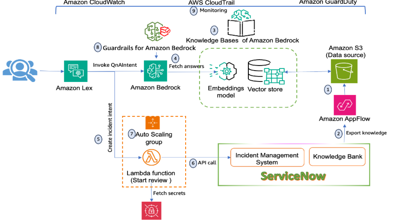
Marcelo Silva is an experienced tech professional who excels in designing, developing, and implementing cutting-edge products. Starting off his career at Cisco, Marcelo worked on various high-profile projects including deployments of the first ever carrier routing system and the successful rollout of ASR9000. His expertise extends to cloud technology, analytics, and product management, having served as senior manager for several companies such as Cisco, Cape Networks, and AWS before joining GenAI. Currently working as a Conversational AI/GenAI Product Manager, Marcelo continues to excel in delivering innovative solutions across industries.

Sujatha Dantuluri is a seasoned Senior Solutions Architect on the US federal civilian team at AWS, with over two decades of experience supporting commercial and federal government clients. Her expertise lies in architecting mission-critical solutions and working closely with customers to ensure their success. Sujatha is an accomplished public speaker, frequently sharing her insights and knowledge at industry events and conferences. She has contributed to IEEE standards and is passionate about empowering others through her engaging presentations and thought-provoking ideas.

NagaBharathi Challa is a solutions architect on the US federal civilian team at Amazon Web Services (AWS). She works closely with customers to effectively use AWS services for their mission use cases, providing architectural best practices and guidance on a wide range of services. Outside of work, she enjoys spending time with family and spreading the power of meditation.

Pranit Raje is a Cloud Architect on the AWS Professional Services India team. He specializes in DevOps, operational excellence, and automation using DevSecOps practices and infrastructure as code. Outside of work, he enjoys going on long drives with his beloved family, spending time with them, and watching movies.

Read More

This post is co-written with Sujith R Pillai from Kyndryl.

In this post, we show you how Kyndryl, an AWS Premier Tier Services Partner and IT infrastructure services provider that designs, builds, manages, and modernizes complex, mission-critical information systems, integrated Amazon Q Business with ServiceNow in a few simple steps. You will learn how to configure Amazon Q Business and ServiceNow, how to create a generative AI plugin for your ServiceNow incidents, and how to test and interact with ServiceNow using the Amazon Q Business web experience. By the end of this post, you will be able to enhance your ServiceNow experience with Amazon Q Business and enjoy the benefits of a generative AI–powered interface.

Solution overview

Amazon Q Business has three main components: a front-end chat interface, a data source connector and retriever, and a ServiceNow plugin. Amazon Q Business uses AWS Secrets Manager secrets to store the ServiceNow credentials securely. The following diagram shows the architecture for the solution.

Chat

Users interact with ServiceNow through the generative AI–powered chat interface using natural language.

Data source connector and retriever

A data source connector is a mechanism for integrating and synchronizing data from multiple repositories into one container index. Amazon Q Business has two types of retrievers: native retrievers and existing retrievers using Amazon Kendra. The native retrievers support a wide range of Amazon Q Business connectors, including ServiceNow. The existing retriever option is for those who already have an Amazon Kendra retriever and would like to use that for their Amazon Q Business application. For the ServiceNow integration, we use the native retriever.

ServiceNow plugin

Amazon Q Business provides a plugin feature for performing actions such as creating incidents in ServiceNow.

The following high-level steps show how to configure the Amazon Q Business – ServiceNow integration:

1. Create a user in ServiceNow for Amazon Q Business to communicate with ServiceNow
2. Create knowledge base articles in ServiceNow if they do not exist already
3. Create an Amazon Q Business application and configure the ServiceNow data source and retriever in Amazon Q Business
4. Synchronize the data source
5. Create a ServiceNow plugin in Amazon Q Business

Prerequisites

To run this application, you must have an Amazon Web Services (AWS) account, an AWS Identity and Access Management (IAM) role, and a user that can create and manage the required resources. If you are not an AWS account holder, see How do I create and activate a new Amazon Web Services account?

You need an AWS IAM Identity Center set up in the AWS Organizations organizational unit (OU) or AWS account in which you are building the Amazon Q Business application. You should have a user or group created in IAM Identity Center. You will assign this user or group to the Amazon Q Business application during the application creation process. For guidance, refer to Manage identities in IAM Identity Center.

You also need a ServiceNow user with incident_manager and knowledge_admin permissions to create and view knowledge base articles and to create incidents. We use a developer instance of ServiceNow for this post as an example. You can find out how to get the developer instance in Personal Developer Instances.

Solution walkthrough

To integrate ServiceNow and Amazon Q Business, use the steps in the following sections.

Create a knowledge base article

Follow these steps to create a knowledge base article:

1. Sign in to ServiceNow and navigate to Self-Service > Knowledge
2. Choose Create an Article
3. On the Create new article page, select a knowledge base and choose a category. Optionally, you may create a new category.
4. Provide a Short description and type in the Article body
5. Choose Submit to create the article, as shown in the following screenshot

Repeat these steps to create a couple of knowledge base articles. In this example, we created a hypothetical enterprise named Example Corp for demonstration purposes.

Create an Amazon Q Business application

Amazon Q offers three subscription plans: Amazon Q Business Lite, Amazon Q Business Pro, and Amazon Q Developer Pro. Read the Amazon Q Documentation for more details. For this example, we used Amazon Q Business Lite.

Create application

Follow these steps to create an application:

1. In the Amazon Q Business console, choose Get started, then choose Create application to create a new Amazon Q Business application, as shown in the following screenshot

2. Name your application in Application name. In Service access, select Create and use a new service-linked role (SLR). For more information about example service roles, see IAM roles for Amazon Q Business. For information on service-linked roles, including how to manage them, see Using service-linked roles for Amazon Q Business. We named our application ServiceNow-Helpdesk. Next, select Create, as shown in the following screenshot.

Choose a retriever and index provisioning

To choose a retriever and index provisioning, follow these steps in the Select retriever screen, as shown in the following screenshot:

1. For Retrievers, select Use native retriever
2. For Index provisioning, choose Starter
3. Choose Next

Connect data sources

Amazon Q Business has ready-made connectors for common data sources and business systems.

1. Enter “ServiceNow” to search and select ServiceNow Online as the data source, as shown in the following screenshot

2. Enter the URL and the version of your ServiceNow instance. We used the ServiceNow version Vancouver for this post.

3. Scroll down the page to provide additional details about the data source. Under Authentication, select Basic authentication. Under AWS Secrets Manager secret, select Create and add a new secret from the dropdown menu as shown in the screenshot.

4. Provide the Username and Password you created in ServiceNow to create an AWS Secrets Manager secret. Choose Save.

5. Under Configure VPC and security group, keep the setting as No VPC because you will be connecting to the ServiceNow by the internet. You may choose to create a new service role under IAM role. This will create a role specifically for this application.

6. In the example, we synchronize the ServiceNow knowledge base articles and incidents. Provide the information as shown in the following image below. Notice that for Filter query the example shows the following code.

workflow_state=published^kb_knowledge_base=dfc19531bf2021003f07e2c1ac0739ab^article_type=text^active=true^EQ

This filter query aims to sync the articles that meet the following criteria:

• workflow_state = published
• kb_knowledge_base = dfc19531bf2021003f07e2c1ac0739ab (This is the default Sys ID for the knowledge base named “Knowledge” in ServiceNow).
• Type = text (This field contains the text in the Knowledge article).
• Active = true (This field filters the articles to sync only the ones that are active).

The filter fields are separated by ^, and the end of the query is represented by EQ. You can find more details about the Filter query and other parameters in Connecting Amazon Q Business to ServiceNow Online using the console.

7. Provide the Sync scope for the Incidents, as shown in the following screenshot

8. You may select Full sync initially so that a complete synchronization is performed. You need to select the frequency of the synchronization as well. For this post, we chose Run on demand. If you need to keep the knowledge base and incident data more up-to-date with the ServiceNow instance, choose a shorter window.

9. A field mapping will be provided for you to validate. You won’t be able to change the field mapping at this stage. Choose Add data source to proceed.

This completes the data source configuration for Amazon Q Business. The configuration takes a few minutes to be completed. Watch the screen for any errors and updates. Once the data source is created, you will be greeted with a message You successfully created the following data source: ‘ServiceNow-Datasource’

Add users and groups

Follow these steps to add users and groups:

1. Choose Next
2. In the Add groups and users page, click Add groups and users. You will be presented with the option of Add and assign new users or Assign existing users and groups. Select Assign existing users and groups. Choose Next, as shown in the following image.

3. Search for an existing user or group in your IAM Identity Center, select one, and choose Assign. After selecting the right user or group, choose Done.

This completes the activity of assigning the user and group access to the Amazon Q Business application.

Create a web experience

Follow these steps to create a web experience in the Add groups and users screen, as shown in the following screenshot.

1. Choose Create and use a new service role in the Web experience service access section
2. Choose Create application

The deployed application with the application status will be shown in the Amazon Q Business > Applications console as shown in the following screenshot.

Synchronize the data source

Once the data source is configured successfully, it’s time to start the synchronization. To begin this process, the ServiceNow fields that require synchronization must be updated. Because we intend to get answers from the knowledge base content, the text field needs to be synchronized. To do so, follow these steps:

1. In the Amazon Q Business console, select Applications in the navigation pane
2. Select ServiceNow-Helpdesk and then ServiceNow-Datasource
3. Choose Actions. From the dropdown, choose Edit, as shown in the following screenshot.

4. Scroll down to the bottom of the page to the Field mappings Select text and description.

5. Choose Update. After the update, choose Sync now.

The synchronization takes a few minutes to complete depending on the amount of data to be synchronized. Make sure that the Status is Completed, as shown in the following screenshot, before proceeding further. If you notice any error, you can choose the error hyperlink. The error hyperlink will take you to Amazon CloudWatch Logs to examining the logs for further troubleshooting.

Create ServiceNow plugin

A ServiceNow plugin in Amazon Q Business helps you create incidents in ServiceNow through Amazon Q Business chat. To create one, follow these steps:

1. In the Amazon Q Business console, select Enhancements from the navigation pane
2. Under Plugins, choose Add plugin, as shown in the following screenshot

3. In the Add Plugin page, shown in the following screenshot, and select the ServiceNow plugin

4. Provide a Name for the plugin
5. Enter the ServiceNow URL and use the previously created AWS Secrets Manager secret for the Authentication
6. Select Create and use a new service role
7. Choose Add plugin

8. The status of the plugin will be shown in the Plugins If Plugin status is Active, the plugin is configured and ready to use.

Use the Amazon Q Business chat interface

To use the Amazon Q Business chat interface, follow these steps:

1. In the Amazon Q Business console, choose Applications from the navigation pane. The web experience URL will be provided for each Amazon Q Business application.

2. Choose the Web experience URL to open the chat interface. Enter an IAM Identity Center username and password that was assigned to this application. The following screenshot shows the Sign in

You can now ask questions and receive responses, as shown in the following image. The answers will be specific to your organization and are retrieved from the knowledge base in ServiceNow.

You can ask the chat interface to create incidents as shown in the next screenshot.

A new pop-up window will appear, providing additional information related to the incident. In this window, you can provide more information related to the ticket and choose Create.

This will create a ServiceNow incident using the web experience of Amazon Q Business without signing in to ServiceNow. You may verify the ticket in the ServiceNow console as shown in the next screenshot.

Conclusion

In this post, we showed how Kyndryl is using Amazon Q Business to enable natural language conversations with ServiceNow using the ServiceNow connector provided by Amazon Q Business. We also showed how to create a ServiceNow plugin that allows users to create incidents in ServiceNow directly from the Amazon Q Business chat interface. We hope that this tutorial will help you take advantage of the power of Amazon Q Business for your ServiceNow needs.

About the authors

Asif Fouzi is a Principal Solutions Architect leading a team of seasoned technologists supporting Global Service Integrators (GSI) such as Kyndryl in their cloud journey. When he is not innovating on behalf of users, he likes to play guitar, travel, and spend time with his family.

Sujith R Pillai is a cloud solution architect in the Cloud Center of Excellence at Kyndryl with extensive experience in infrastructure architecture and implementation across various industries. With his strong background in cloud solutions, he has led multiple technology transformation projects for Kyndryl customers.

Read More

This post introduces HCLTech’s AutoWise Companion, a transformative generative AI solution designed to enhance customers’ vehicle purchasing journey. By tailoring recommendations based on individuals’ preferences, the solution guides customers toward the best vehicle model for them. Simultaneously, it empowers vehicle manufacturers (original equipment manufacturers (OEMs)) by using real customer feedback to drive strategic decisions, boosting sales and company profits. Powered by generative AI services on AWS and large language models’ (LLMs’) multi-modal capabilities, HCLTech’s AutoWise Companion provides a seamless and impactful experience.

In this post, we analyze the current industry challenges and guide readers through the AutoWise Companion solution functional flow and architecture design using built-in AWS services and open source tools. Additionally, we discuss the design from security and responsible AI perspectives, demonstrating how you can apply this solution to a wider range of industry scenarios.

Opportunities

Purchasing a vehicle is a crucial decision that can induce stress and uncertainty for customers. The following are some of the real-life challenges customers and manufacturers face:

• Choosing the right brand and model – Even after narrowing down the brand, customers must navigate through a multitude of vehicle models and variants. Each model has different features, price points, and performance metrics, making it difficult to make a confident choice that fits their needs and budget.
• Analyzing customer feedback – OEMs face the daunting task of sifting through extensive quality reporting tool (QRT) reports. These reports contain vast amounts of data, which can be overwhelming and time-consuming to analyze.
• Aligning with customer sentiments – OEMs must align their findings from QRT reports with the actual sentiments of customers. Understanding customer satisfaction and areas needing improvement from raw data is complex and often requires advanced analytical tools.

HCLTech’s AutoWise Companion solution addresses these pain points, benefiting both customers and manufacturers by simplifying the decision-making process for customers and enhancing data analysis and customer sentiment alignment for manufacturers.

The solution extracts valuable insights from diverse data sources, including OEM transactions, vehicle specifications, social media reviews, and OEM QRT reports. By employing a multi-modal approach, the solution connects relevant data elements across various databases. Based on the customer query and context, the system dynamically generates text-to-SQL queries, summarizes knowledge base results using semantic search, and creates personalized vehicle brochures based on the customer’s preferences. This seamless process is facilitated by Retrieval Augmentation Generation (RAG) and a text-to-SQL framework.

Solution overview

The overall solution is divided into functional modules for both customers and OEMs.

Customer assist

Every customer has unique preferences, even when considering the same vehicle brand and model. The solution is designed to provide customers with a detailed, personalized explanation of their preferred features, empowering them to make informed decisions. The solution presents the following capabilities:

• Natural language queries – Customers can ask questions in plain language about vehicle features, such as overall ratings, pricing, and more. The system is equipped to understand and respond to these inquiries effectively.
• Tailored interaction – The solution allows customers to select specific features from an available list, enabling a deeper exploration of their preferred options. This helps customers gain a comprehensive understanding of the features that best suit their needs.
• Personalized brochure generation – The solution considers the customer’s feature preferences and generates a customized feature explanation brochure (with specific feature images). This personalized document helps the customer gain a deeper understanding of the vehicle and supports their decision-making process.

OEM assist

OEMs in the automotive industry must proactively address customer complaints and feedback regarding various automobile parts. This comprehensive solution enables OEM managers to analyze and summarize customer complaints and reported quality issues across different categories, thereby empowering them to formulate data-driven strategies efficiently. This enhances decision-making and competitiveness in the dynamic automotive industry. The solution enables the following:

• Insight summaries – The system allows OEMs to better understand the insightful summary presented by integrating and aggregating data from various sources, such as QRT reports, vehicle transaction sales data, and social media reviews.
• Detailed view – OEMs can seamlessly access specific details about issues, reports, complaints, or data point in natural language, with the system providing the relevant information from the referred reviews data, transaction data, or unstructured QRT reports.

To better understand the solution, we use the seven steps shown in the following figure to explain the overall function flow.

The overall function flow consists of the following steps:

1. The user (customer or OEM manager) interacts with the system through a natural language interface to ask various questions.
2. The system’s natural language interpreter, powered by a generative AI engine, analyzes the query’s context, intent, and relevant persona to identify the appropriate data sources.
3. Based on the identified data sources, the respective multi-source query execution plan is generated by the generative AI engine.
4. The query agent parses the execution plan and send queries to the respective query executor.
5. Requested information is intelligently fetched from multiple sources such as company product metadata, sales transactions, OEM reports, and more to generate meaningful responses.
6. The system seamlessly combines the collected information from the various sources, applying contextual understanding and domain-specific knowledge to generate a well-crafted, comprehensive, and relevant response for the user.
7. The system generates the response for the original query and empowers the user to continue the interaction, either by asking follow-up questions within the same context or exploring new areas of interest, all while benefiting from the system’s ability to maintain contextual awareness and provide consistently relevant and informative responses.

Technical architecture

The overall solution is implemented using AWS services and LangChain. Multiple LangChain functions, such as CharacterTextSplitter and embedding vectors, are used for text handling and embedding model invocations. In the application layer, the GUI for the solution is created using Streamlit in Python language. The app container is deployed using a cost-optimal AWS microservice-based architecture using Amazon Elastic Container Service (Amazon ECS) clusters and AWS Fargate.

The solution contains the following processing layers:

• Data pipeline – The various data sources, such as sales transactional data, unstructured QRT reports, social media reviews in JSON format, and vehicle metadata, are processed, transformed, and stored in the respective databases.
• Vector embedding and data cataloging – To support natural language query similarity matching, the respective data is vectorized and stored as vector embeddings. Additionally, to enable the natural language to SQL (text-to-SQL) feature, the corresponding data catalog is generated for the transactional data.
• LLM (request and response formation) – The system invokes LLMs at various stages to understand the request, formulate the context, and generate the response based on the query and context.
• Frontend application – Customers or OEMs interact with the solution using an assistant application designed to enable natural language interaction with the system.

The solution uses the following AWS data stores and analytics services:

• Unstructured data – Amazon Simple Storage Service (Amazon S3) buckets are used to store the JSON-based social media feedback data, quality report PDFs (specific to OEMs), and the vehicle and its features images.
• Transactional sales data – Amazon Relational Database Service (Amazon RDS) for PostgreSQL is used to hold transactional reports of vehicles on a quarterly or monthly basis.
• Vehicle specification data – Amazon DynamoDB is used to store the vehicle metadata (its features and specifications).
• Amazon Athena – Amazon Athena is used to query the JSON-based social media feedback data stored in an S3 bucket.
• AWS Glue – AWS Glue is used for data cataloging.

The following figure depicts the technical flow of the solution.

The workflow consists of the following steps:

1. The user’s query, expressed in natural language, is processed by an orchestrated AWS Lambda
2. The Lambda function tries to find the query match from the LLM cache. If a match is found, the response is returned from the LLM cache. If no match is found, the function invokes the respective LLMs through Amazon Bedrock. This solution uses LLMs (Anthropic’s Claude 2 and Claude 3 Haiku) on Amazon Bedrock for response generation. The Amazon Titan Embeddings G1 – Text LLM is used to convert the knowledge documents and user queries into vector embeddings.
3. Based on the context of the query and the available catalog, the LLM identifies the relevant data sources:
   1. The transactional sales data, social media reviews, vehicle metadata, and more, are transformed and used for customers and OEM interactions.
   2. The data in this step is restricted and is only accessible for OEM personas to help diagnose the quality related issues and provide insights on the QRT reports. This solution uses Amazon Textract as a data extraction tool to extract text from PDFs (such as quality reports).
4. The LLM generates queries (text-to-SQL) to fetch data from the respective data channels according to the identified sources.
5. The responses from each data channel are assembled to generate the overall context.
6. Additionally, to generate a personalized brochure, relevant images (described as text-based embeddings) are fetched based on the query context. Amazon OpenSearch Serverless is used as a vector database to store the embeddings of text chunks extracted from quality report PDFs and image descriptions.
7. The overall context is then passed to a response generator LLM to generate the final response to the user. The cache is also updated.

Responsible generative AI and security considerations

Customers implementing generative AI projects with LLMs are increasingly prioritizing security and responsible AI practices. This focus stems from the need to protect sensitive data, maintain model integrity, and enforce ethical use of AI technologies. The AutoWise Companion solution uses AWS services to enable customers to focus on innovation while maintaining the highest standards of data protection and ethical AI use.

Amazon Bedrock Guardrails

Amazon Bedrock Guardrails provides configurable safeguards that can be applied to user input and foundation model output as safety and privacy controls. By incorporating guardrails, the solution proactively steers users away from potential risks or errors, promoting better outcomes and adherence to established standards. In the automobile industry, OEM vendors usually apply safety filters for vehicle specifications. For example, they want to validate the input to make sure that the queries are about legitimate existing models. Amazon Bedrock Guardrails provides denied topics and contextual grounding checks to make sure the queries about non-existent automobile models are identified and denied with a custom response.

Security considerations

The system employs a RAG framework that relies on customer data, making data security the foremost priority. By design, Amazon Bedrock provides a layer of data security by making sure that customer data stays encrypted and protected and is neither used to train the underlying LLM nor shared with the model providers. Amazon Bedrock is in scope for common compliance standards, including ISO, SOC, CSA STAR Level 2, is HIPAA eligible, and customers can use Amazon Bedrock in compliance with the GDPR.

For raw document storage on Amazon S3, transactional data storage, and retrieval, these data sources are encrypted, and respective access control mechanisms are put in place to maintain restricted data access.

Key learnings

The solution offered the following key learnings:

• LLM cost optimization – In the initial stages of the solution, based on the user query, multiple independent LLM calls were required, which led to increased costs and execution time. By using the AWS Glue Data Catalog, we have improved the solution to use a single LLM call to find the best source of relevant information.
• LLM caching – We observed that a significant percentage of queries received were repetitive. To optimize performance and cost, we implemented a caching mechanism that stores the request-response data from previous LLM model invocations. This cache lookup allows us to retrieve responses from the cached data, thereby reducing the number of calls made to the underlying LLM. This caching approach helped minimize cost and improve response times.
• Image to text – Generating personalized brochures based on customer preferences was challenging. However, the latest vision-capable multimodal LLMs, such as Anthropic’s Claude 3 models (Haiku and Sonnet), have significantly improved accuracy.

Industrial adoption

The aim of this solution is to help customers make an informed decision while purchasing vehicles and empowering OEM managers to analyze factors contributing to sales fluctuations and formulate corresponding targeted sales boosting strategies, all based on data-driven insights. The solution can also be adopted in other sectors, as shown in the following table.

Conclusion

The solution discussed in this post demonstrates the power of generative AI on AWS by empowering customers to use natural language conversations to obtain personalized, data-driven insights to make informed decisions during the purchase of their vehicle. It also supports OEMs in enhancing customer satisfaction, improving features, and driving sales growth in a competitive market.

Although the focus of this post has been on the automotive domain, the presented approach holds potential for adoption in other industries to provide a more streamlined and fulfilling purchasing experience.

Overall, the solution demonstrates the power of generative AI to provide accurate information based on various structured and unstructured data sources governed by guardrails to help avoid unauthorized conversations. For more information, see the HCLTech GenAI Automotive Companion in AWS Marketplace.

About the Authors

Bhajan Deep Singh leads the AWS Gen AI/AIML Center of Excellence at HCL Technologies. He plays an instrumental role in developing proof-of-concept projects and use cases utilizing AWS’s generative AI offerings. He has successfully led numerous client engagements to deliver data analytics and AI/machine learning solutions. He holds AWS’s AI/ML Specialty, AI Practitioner certification and authors technical blogs on AI/ML services and solutions. With his expertise and leadership, he enables clients to maximize the value of AWS generative AI.

Mihir Bhambri works as AWS Senior Solutions Architect at HCL Technologies. He specializes in tailored Generative AI solutions, driving industry-wide innovation in sectors such as Financial Services, Life Sciences, Manufacturing, and Automotive. Leveraging AWS cloud services and diverse Large Language Models (LLMs) to develop multiple proof-of-concepts to support business improvements. He also holds AWS Solutions Architect Certification and has contributed to the research community by co-authoring papers and winning multiple AWS generative AI hackathons.

Yajuvender Singh is an AWS Senior Solution Architect at HCLTech, specializing in AWS Cloud and Generative AI technologies. As an AWS-certified professional, he has delivered innovative solutions across insurance, automotive, life science and manufacturing industries and also won multiple AWS GenAI hackathons in India and London. His expertise in developing robust cloud architectures and GenAI solutions, combined with his contributions to the AWS technical community through co-authored blogs, showcases his technical leadership.

Sara van de Moosdijk, simply known as Moose, is an AI/ML Specialist Solution Architect at AWS. She helps AWS partners build and scale AI/ML solutions through technical enablement, support, and architectural guidance. Moose spends her free time figuring out how to fit more books in her overflowing bookcase.

Jerry Li, is a Senior Partner Solution Architect at AWS Australia, collaborating closely with HCLTech in APAC for over four years. He also works with HCLTech Data & AI Center of Excellence team, focusing on AWS data analytics and generative AI skills development, solution building, and go-to-market (GTM) strategy.

About HCLTech

HCLTech is at the vanguard of generative AI technology, using the robust AWS Generative AI tech stack. The company offers cutting-edge generative AI solutions that are poised to revolutionize the way businesses and individuals approach content creation, problem-solving, and decision-making. HCLTech has developed a suite of readily deployable generative AI assets and solutions, encompassing the domains of customer experience, software development life cycle (SDLC) integration, and industrial processes.

Read More