Posts in category: Amazon AWS

In April 2020, AWS and Facebook announced the launch of TorchServe to allow researches and machine learning (ML) developers from the PyTorch community to bring their models to production more quickly and without needing to write custom code. TorchServe is an open-source project that answers the industry question of how to go from a notebook to production using PyTorch and customers around the world, such as Matroid, are experiencing the benefits firsthand. Similarly, over 10,000 customers have adopted Amazon SageMaker to quickly build, train, and deploy ML models at scale, and many of them have made it their standard platform for ML. From a model serving perspective, Amazon SageMaker abstracts all the infrastructure-centric heavy lifting and allows you to deliver low-latency predictions securely and reliably to millions of concurrent users around the world.

TorchServe’s native integration with Amazon SageMaker

AWS is excited to announce that TorchServe is now natively supported in Amazon SageMaker as the default model server for PyTorch inference. Previously, you could use TorchServe with Amazon SageMaker by installing it on a notebook instance and starting a server to perform local inference or by building a TorchServe container and referencing its image to create a hosted endpoint. However, full notebook installations can be time-intensive and some data scientists and ML developers may not prefer to manage all the steps and AWS Identity and Access Management (IAM) permissions involved with building the Docker container and storing the image on Amazon Elastic Container Registry (Amazon ECR) before ultimately uploading the model to Amazon Simple Storage Service (Amazon S3) and deploying the model endpoint. With this release, you can use the native Amazon SageMaker SDK to serve PyTorch models with TorchServe.

To support TorchServe natively in Amazon SageMaker, the AWS engineering teams submitted pull requests to the aws/sagemaker-pytorch-inference-toolkit and the aws/deep-learning-containers repositories. After these were merged, we could use TorchServe via the Amazon SageMaker APIs for PyTorch inference. This change introduces a tighter integration with the PyTorch community. As more features related to the TorchServe serving framework are released in the future, they are tested, ported over, and made available as an AWS Deep Learning Container image. It’s important to note that our implementation hides the .mar from the user while still using the Amazon SageMaker PyTorch API everyone is used to.

The TorchServe architecture in Amazon SageMaker

You can use TorchServe natively with Amazon SageMaker through the following steps:

1. Create a model in Amazon SageMaker. By creating a model, you tell Amazon SageMaker where it can find the model components. This includes the Amazon S3 path where the model artifacts are stored and the Docker registry path for the Amazon SageMaker TorchServe image. In subsequent deployment steps, you specify the model by name. For more information, see CreateModel.
2. Create an endpoint configuration for an HTTPS endpoint. You specify the name of one or more models in production variants and the ML compute instances that you want Amazon SageMaker to launch to host each production variant. When hosting models in production, you can configure the endpoint to elastically scale the deployed ML compute instances. For each production variant, you specify the number of ML compute instances that you want to deploy. When you specify two or more instances, Amazon SageMaker launches them in multiple Availability Zones. This provides continuous availability. Amazon SageMaker manages deploying the instances. For more information, see CreateEndpointConfig.
3. Create an HTTPS endpoint. Provide the endpoint configuration to Amazon SageMaker. The service launches the ML compute instances and deploys the model or models as specified in the configuration. For more information, see CreateEndpoint. To get inferences from the model, client applications send requests to the Amazon SageMaker Runtime HTTPS endpoint. For more information about the API, see InvokeEndpoint.

The Amazon SageMaker Python SDK simplifies these steps as we will demonstrate in the following example notebook.

Using a fine-tuned HuggingFace base transformer (RoBERTa)

For this post, we use a HuggingFace transformer, which provides us with a general-purpose architecture for Natural Language Understanding (NLU). Specifically, we present you with a RoBERTa base transformer that was fined tuned to perform sentiment analysis. The pre-trained checkpoint loads the additional head layers and the model will outputs positive, neutral, and negative sentiment of text.

Deploying a CloudFormation Stack and verifying notebook creation

You will deploy an ml.m5.xlarge Amazon SageMaker notebook instance. For more information about pricing, see Amazon SageMaker Pricing.

1. Sign in to the AWS Management Console.
2. Choose from the following table to launch your template.

Launch Template	Region
	N.Virginia (us-east-1)
	Ireland (eu-west-1)
	Singapore (ap-southeast-1)

You can launch this stack for any Region by updating the hyperlink’s Region value.

3. In the Capabilities and transforms section, select the three acknowledgement boxes.
4. Choose Create stack.

Your CloudFormation stack takes about 5 minutes to complete creating the Amazon SageMaker notebook instance and its IAM role.

5. When the stack creation is complete, check the output on the Resources tab.
   
6. On the Amazon SageMaker console, under Notebook, choose Notebook instances.
7. Locate your newly created notebook and choose Open Jupyter.
   

Accessing the Lab

From within the notebook instance, navigate to the serving_natively_with_amazon_sagemaker directory and open deploy.ipynb.

You can now run through the steps within the Jupyter notebook:

1. Set up your hosting environment.
2. Create your endpoint.
3. Perform predictions with a TorchServe backend Amazon SageMaker endpoint.

After setting up your hosting environment, creating an Amazon SageMaker endpoint using the native TorchServe estimator is as easy as:

model = PyTorchModel(model_data=model_artifact,
                   name=name_from_base('roberta-model'),
                   role=role, 
                   entry_point='torchserve-predictor.py',
                   source_dir='source_dir',
                   framework_version='1.6.0',
                   predictor_cls=SentimentAnalysis)

endpoint_name = name_from_base('roberta-model')
predictor = model.deploy(initial_instance_count=1, instance_type='ml.m5.xlarge', endpoint_name=endpoint_name)

Cleaning Up

When you’re finished with this lab, your Amazon SageMaker endpoint should have already been deleted. If not, complete the following steps to delete it:

1. On the Amazon SageMaker console, under Inference, choose Endpoints.
2. Select the endpoint (it should begin with roberta-model).
3. From the Actions drop-down menu, choose Delete.

On the AWS CloudFormation console, delete the rest of your environment choosing the torchserve-on-aws stack and choosing Delete.

You can see two other stack names that were built based off of the original CloudFormation template. These are nested stacks and are automatically deleted with the main stack. The cleanup process takes just over 3 minutes to spin down your environment and will delete your notebook instance and the associated IAM role.

Conclusion

As TorchServe continues to evolve around the very specific needs of the PyTorch community, AWS is focused on ensuring that you have a common and performant way to serve models with PyTorch. Whether you’re using Amazon SageMaker, Amazon Elastic Compute Cloud (Amazon EC2), or Amazon Elastic Kubernetes Service (Amazon EKS), you can expect AWS to continue to optimize the backend infrastructure in support of our open-source community. We encourage all of you to submit pull requests and/or create issues in our repositories (TorchServe, AWS Deep learning containers, PyTorch inference toolkit, etc) as needed.

About the Author

As a Principal Solutions Architect, Todd spends his time working with strategic and global customers to define business requirements, provide architectural guidance around specific use cases, and design applications and services that are scalable, reliable, and performant. He has helped launch and scale the reinforcement learning powered AWS DeepRacer service, is a host for the AWS video series “This is My Architecture”, and speaks regularly at AWS re:Invent, AWS Summits, and technology conferences around the world.

Read More

Live video streams are continuously generated across industries including media and entertainment, retail, and many more. Live events like sports, music, news, and other special events are broadcast for viewers on TV and other online streaming platforms.

AWS customers increasingly rely on machine learning (ML) to generate actionable insights in real time and deliver an enhanced viewing experience or timely alert notifications. For example, AWS Sports explains how leagues, broadcasters, and partners can train teams, engage fans, and transform the business of sports with ML.

Amazon Rekognition makes it easy to add image and video analysis to your applications using proven, highly scalable, deep learning technology that requires no ML expertise to use. With Amazon Rekognition, you can identify objects, people, text, scenes, and some pre-defined activities in videos.

However, if you want to use your own video activity dataset and your own model or algorithm, you can use Amazon SageMaker. Amazon SageMaker is a fully managed service that allows you to build, train, and deploy ML models quickly. Amazon SageMaker removes the heavy lifting from each step of the ML process to make it easier to develop high-quality models.

In this post, you use Amazon SageMaker to automatically detect activities from a custom dataset in a live video stream.

The large volume of live video streams generated needs to be stored, processed in real time, and reviewed by a human team at low latency and low cost. Such pipelines include additional processing steps if specific activities are automatically detected in a video segment, such as penalty kicks in football triggering the generation of highlight clips for viewer replay.

ML inference on a live video stream can have the following challenges:

• Input source – The live stream video input must be segmented and made available in a data store for consumption with negligible latency.
• Large payload size – A video segment of 10 seconds can range from 1–15 MB. This is significantly larger than a typical tabular data record.
• Frame sampling – Video frames must be extracted at a sampling rate generally lesser than the original video FPS (frames per second) efficiently and without a loss in output accuracy.
• Frame preprocessing – Video frames must be preprocessed to reduce image size and resolution without a loss in output accuracy. They also need to be normalized across all the images used in training.
• External dependencies – External libraries like opencv and ffmpeg with different license types are generally used for image processing.
• 3D model network – Video models are typically 3D networks with an additional temporal dimension to image networks. They work on 5D input (batch size, time, RGB channel, height, width) and require a large volume of annotated input videos.
• Low latency, low cost – The output ML inference needs to be generated within an acceptable latency and at a low cost to demonstrate value.

This post describes two phases of a ML lifecycle. In the first phase, you build, train, and deploy a 3D video classification model on Amazon SageMaker. You fine-tune a pre-trained model with a ResNet50 backbone by transfer learning on another dataset and test inference on a sample video segment. The pre-trained model from a well-known model zoo reduces the need for large volumes of annotated input videos and can be adapted for tasks in another domain.

In the second phase, you deploy the fine-tuned model on an Amazon SageMaker endpoint in a production context of an end-to-end solution with a live video stream. The live video stream is simulated by a sample video in a continuous playback loop with AWS Elemental MediaLive. Video segments from the live stream are delivered to Amazon Simple Storage Service (Amazon S3), which invokes the Amazon SageMaker endpoint for inference. The inference payload is the Amazon S3 URI of the video segment. The use of the Amazon S3 URI is efficient because it eliminates the need to serialize and deserialize a large video frame payload over a REST API and transfers the responsibility of ingesting the video to the endpoint. The endpoint inference performs frame sampling and pre-processing followed by video segment classification, and outputs the result to Amazon DynamoDB.

Finally, the solution performance is summarized with respect to latency, throughput, and cost.

For the complete code associated with this post, see the GitHub repo.

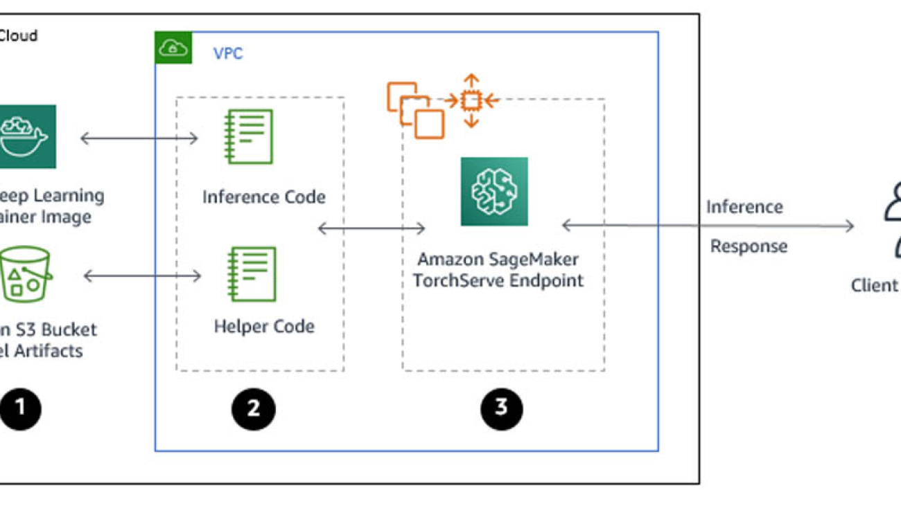
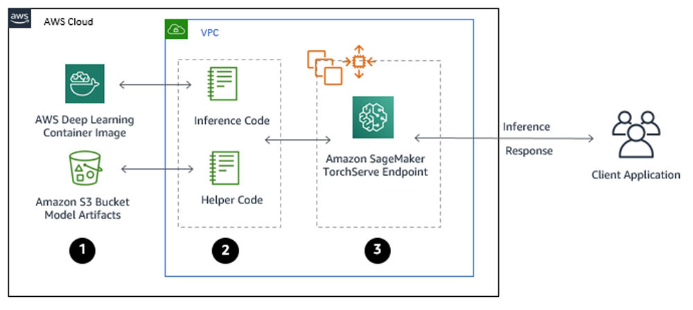
Building, training, and deploying an activity detection model with Amazon SageMaker

In this section, you use Amazon SageMaker to build, train, and deploy an activity detection model in a development environment. The following diagram depicts the Amazon SageMaker ML pipeline used to perform the end-to-end model development. The training and inference Docker images are available for any deep learning framework of choice, like TensorFlow, Pytorch, and MXNet. You use the “bring your own script” capability of Amazon SageMaker to provide a custom entrypoint script for training and inference. For this use case, you use transfer learning to fine-tune a pretrained model from a model zoo with another dataset loaded in Amazon S3. You use model artifacts from the training job to deploy an endpoint with automatic scaling, which dynamically adjusts the number of instances in response to changes in the invocation workload.

For this use case, you use two popular activity detection datasets: Kinetics400 and UCF101. Dataset size is a big factor in the performance of deep learning models. Kinetics400 has 306,245 short trimmed videos from 400 action categories. However, you may not have such a high volume of annotated videos in other domains. Training a deep learning model on small datasets from scratch may lead to severe overfitting, which is why you need transfer learning.

UCF101 has 13,320 videos from 101 action categories. For this post, we use UCF101 as a dataset from another domain for transfer learning. The pre-trained model is fine-tuned by replacing the last classification (dense) layer to the number of classes in the UCF101 dataset. The final test inference is run on new sample videos from Pexels that were unavailable during the training phase. Similarly, you can train good models on activity videos from your own domain without large annotated datasets and with less computing resource utilization.

We chose Apache MXNet as the deep learning framework for this use case because of the availability of the GluonCV toolkit. GluonCV provides implementations of state-of-the-art deep learning algorithms in computer vision. It features training scripts that reproduce state-of-the-art results reported in the latest research papers, a model zoo with a large set of pre-trained models, carefully designed APIs, and easy-to-understand implementations and community support. The action recognition model zoo contains multiple pre-trained models with the Kinetics400 dataset. The following graph shows the inference throughputs vs. validation accuracy and device memory footprint for each of them.

I3D (Inflated 3D Networks) and SlowFast are 3D video classification networks with varying trade-offs between accuracy and efficiency. For this post, we chose the Inflated 3D model (I3D) with ResNet50 backbone trained on the Kinetics400 dataset. It uses 3D convolution to learn spatiotemporal information directly from videos. The input to this model is of the form (N x C x T x H x W), where N is the batch size, C is the number of colour channels, T is the number of frames in the video segment, H is the height of the video frame, and W is the width of the video frame.

Both model training and inference require efficient and convenient slicing methods for video preprocessing. Decord provides such methods based on a thin wrapper on top of hardware accelerated video decoders. We use Decord as a video reader, and use VideoClsCustom as a custom GluonCV video data loader for pre-processing.

We launch the training script mode with the Amazon SageMaker MXNet training toolkit and the AWS Deep Learning container for training on Apache MXNet. The training process includes the following steps for the entire dataset:

• Frame sampling and center cropping
• Frame normalization with mean and standard deviation across all ImageNet images
• Transfer learning on the pre-trained model with a new dataset

After you have a trained model artifact, you can include it in a Docker container that runs your inference script and deploys to an Amazon SageMaker endpoint. Inference is launched with the Amazon SageMaker MXNet inference toolkit and the AWS Deep Learning container for inference on Apache MXNet. The inference process includes the following steps for the video segment payload:

• Pre-processing (similar to training)
• Activity classification

We use the Amazon Elastic Compute Cloud (Amazon EC2) G4 instance for our Amazon SageMaker endpoint hosting. G4 instances provide the latest generation NVIDIA T4 GPUs, AWS custom Intel Cascade Lake CPUs, up to 100 Gbps of networking throughput, and up to 1.8 TB of local NVMe storage. G4 instances are optimized for computer vision application deployments like image classification and object detection. For more information about inference benchmarks, see NVIDIA Data Center Deep Learning Product Performance.

We test the model inference deployed as an Amazon SageMaker endpoint using the following video examples (included in the code repository).

Output activity  : TennisSwing

Output activity  : Skiing

Note that the UCF101 dataset does not have a snowboarding activity class. The most similar activity present in the dataset is skiing and the model predicts skiing when evaluated with a snowboarding video.

You can find the complete Amazon SageMaker Jupyter notebook example with transfer learning and inference on the GitHub repo. After the model is trained, deployed to an Amazon SageMaker endpoint, and tested with the sample videos in the development environment, you can deploy it in a production context of an end-to-end solution.

Deploying the solution with AWS CloudFormation

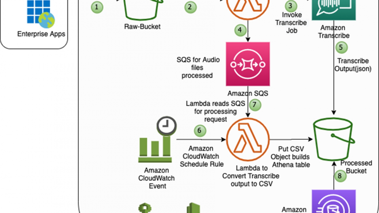
In this step, you deploy the end-to-end activity detection solution using an AWS CloudFormation template. After a successful deployment, you use the model to automatically detect an activity in a video segment from a live video stream. The following diagram depicts the roles of the AWS services in the solution.

The AWS Elemental MediaLive livestreaming channel that is created from a sample video file in S3 bucket is used to demonstrate the real-time architecture. You can use other live streaming services as well that are capable of delivering live video segments to S3.

1. AWS Elemental MediaLive sends live video with HTTP Live Streaming (HLS) and regularly generates fragments of equal length (10 seconds) as .ts files and an index file that contains references of the fragmented files as a .m3u8 file in a S3 bucket.
2. An upload of each video .ts fragment into the S3 bucket triggers a lambda function.
3. The lambda function simply invokes a SageMaker endpoint for activity detection with the S3 URI of the video fragment as the REST API payload input.
4. The SageMaker inference container reads the video from S3, pre-processes it, detects an activity and saves the prediction results to an Amazon DynamoDB table.

For this post, we use the sample Skiing People video to create the MediaLive live stream channel (also included in the code repository). In addition, the deployed model is the I3D model with Resnet50 backbone fine-tuned with the UCF101 dataset, as explained in the previous section. Autoscaling is enabled for the Amazon SageMaker endpoint to adjust the number of instances based on the actual workload.

The end-to-end solution example is provided in the GitHub repo. You can also use your own sample video and fine-tuned model.

There is a cost associated with deploying and running the solution, as mentioned in the Cost Estimation section of this post. Make sure to delete the CloudFormation stack if you no longer need it. The steps to delete the solution are detailed in the section Cleaning up.

You can deploy the solution by launching the CloudFormation stack:

The solution is deployed in the us-east-1 Region. For instructions on changing your Region, see the GitHub repo. After you launch the CloudFormation stack, you can update the parameters for your environments or leave the defaults. All their descriptions are provided when you launch it. Don’t create or select any other options in the configuration. In addition, don’t create or select an AWS Identity and Access Management (IAM) role on the Permissions tab. At the final page of the CloudFormation creation process, you need to select the two check-boxes under Capabilities. To create the AWS resources associated with the solution, you should have permissions to create CloudFormation stacks.

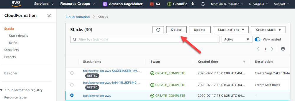
After you launch the stack, make sure that the root stack with its nested sub-stacks are successfully created by viewing the stack on the AWS CloudFormation console.

Wait until all the stacks are successfully created before you proceed to the next session. It takes 15–20 minutes to deploy the architecture.

The root CloudFormation stack ActivityDetectionCFN is mainly used to call the other nested sub-stacks and create the corresponding AWS resources.

The sub-stacks have the root stack name as their prefix. This is mainly to show that they are nested. In addition, the AWS Region name and account ID are added as suffices in the live stream S3 bucket name to avoid naming conflicts.

After the solution is successfully deployed, the following AWS resources are created:

• S3 bucket – The bucket activity-detection-livestream-bucket-us-east-1-<account-id> stores video segments from the live video stream
• MediaLive channel – The channel activity-detection-channel creates video segments from the live video stream and saves them to the S3 bucket
• Lambda function – The function activity-detection-lambda invokes the Amazon SageMaker endpoint to detect activities from each video segment
• SageMaker endpoint – The endpoint activity-detection-endpoint loads a video segment, detects an activity, and saves the results into a DynamoDB table
• DynamoDB table – The table activity-detection-table stores the prediction results from the endpoint

Other supporting resources, like IAM roles, are also created to provide permissions to their respective resources.

Using the Solution

After the solution is successfully deployed, it’s time to test the model with a live video stream. You can start the channel on the MediaLive console.

Wait for the channel state to change to Running. When the channel state changes to Running, .ts-formatted video segments are saved into the live stream S3 bucket.

Only the most recent 21 video segments are kept in the S3 bucket to save storage. For more information about increasing the number of segments, see the GitHub repo.

Each .ts-formatted video upload triggers a Lambda function. The function invokes the Amazon SageMaker endpoint with an Amazon S3 URI to the .ts video as the payload. The deployed model predicts the activity and saves the results to the DynamoDB table.

Evaluating performance results

The Amazon SageMaker endpoint instance in this post is a ml.g4dn.2xlarge with 8 vCPU and 1 Nvidia T4 Tensor Core GPU. The solution generates one video segment every 10 seconds at 30 FPS. Therefore, there are six endpoint requests per minute (RPM). The overhead latency in video segment creation from the live stream up to delivery in Amazon S3 is approximately 1 second.

Amazon SageMaker supports automatic scaling for your hosted models. Autoscaling dynamically adjusts the number of instances provisioned for a model in response to changes in your workload. You can simulate a load test to determine the throughput of the system and the scaling policy for autoscaling in Amazon SageMaker. For the activity detection model in this post, a single ml.g4dn.2xlarge instance hosting the endpoint can handle 600 RPM with a latency of 300 milliseconds and with less than 5% number of HTTP errors. With a SAFETY_FACTOR = 0.5, the autoscaling target metric can be set as SageMakerVariantInvocationsPerInstance = 600 * 0.5 = 300 RPM.

For more information on load testing, see Load testing your autoscaling configuration.

Observe the differences between two scenarios under the same increasing load up to 1,700 invocations per minute in a period of 15 minutes. The BEFORE scenario is for a single instance without autoscaling, and the AFTER scenario is after two additional instances are launched by autoscaling.

The following graphs report the number of invocations and invocations per instance per minute. In the BEFORE scenario, with a single instance, both lines merge. In the AFTER scenario, the load pattern and Invocations (the blue line) are similar, but InvocationsPerInstance (the red line) is lower because the endpoint has scaled out.

The following graphs report average ModelLatency per minute. In the BEFORE scenario, the average latency remains under 300 milliseconds for the first 3 minutes of the test. The average ModelLatency exceeds 1 second after the endpoint gets more than 600 RPS and goes up to 8 seconds during peak load. In the AFTER scenario, the endpoint has already scaled to three instances and the average ModelLatency per minute remains close to 300 milliseconds.

The following graphs report the errors from the endpoint. In the BEFORE scenario, as the load exceeds 300 RPS, the endpoint starts to error out for some requests and increases as the number of invocations increase. In the AFTER scenario, the endpoint has scaled out already and reports no errors.

In the AFTER scenario, at peak load, average CPU utilization across instances is near maximum (100 % * 8 vcpu = 800 %) and average GPU utilization across instances is about 35%. To improve GPU utilization, additional effort can be made to optimize the CPU intensive pre-processing.

Cost Estimation

The following table summarizes the cost estimation for this solution. The cost includes the per hour pricing for one Amazon SageMaker endpoint instance of type ml.g4dn.2xlarge in the us-east-1 Region. If autoscaling is applied, the cost per hour includes the cost of the number of active instances. Also, MediaLive channel pricing is governed by the input and output configuration for the channel.

Cleaning up

If you no longer need the solution, complete the following steps to properly delete all the associated AWS resources:

1. On the MediaLive console, stop the live stream channel.
2. On the Amazon S3 console, delete the S3 bucket you created earlier.
3. On the AWS CloudFormation console, delete the root ActivityDetectionCFN This also removes all nested sub-stacks.

Conclusion

In this post, you used Amazon SageMaker to automatically detect activity in a simulated live video stream. You used a pre-trained model from the gluon-cv model zoo and Apache MXNet framework for transfer learning on another dataset. You also used Amazon SageMaker inference to preprocess and classify a video segment delivered to Amazon S3. Finally, you evaluated the solution respect to model latency, system throughput, and cost.

About the Authors

Hasan Poonawala is a Machine Learning Specialist Solution Architect at AWS, based in London, UK. Hasan helps customers design and deploy machine learning applications in production on AWS. He is passionate about the use of machine learning to solve business problems across various industries. In his spare time, Hasan loves to explore nature outdoors and spend time with friends and family.

Tesfagabir Meharizghi is a Data Scientist at the Amazon ML Solutions Lab where he works with customers across different verticals accelerate their use of machine learning and AWS cloud services to solve their business challenges. Outside of work, he enjoys spending time with his family and reading books.

Read More

In an effort to drive customer service improvements, many companies record the phone conversations between their customers and call center representatives. These call recordings are typically stored as audio files and processed to uncover insights such as customer sentiment, product or service issues, and agent effectiveness. To provide an accurate analysis of these audio files, the transcriptions need to clearly identify who spoke what and when.

However, given the average customer service agent handles 30–50 calls a day, the sheer volume of audio files to analyze quickly becomes a challenge. Companies need a robust system for transcribing audio files in large batches to improve call center quality management. Similarly, legal investigations often need to efficiently analyze case-related audio files in search of potential evidence or insight that can help win legal cases. Also, in the healthcare sector, there is a growing need for this solution to help transcribe and analyze virtual patient-provider interactions.

Amazon Transcribe is an automatic speech recognition (ASR) service that makes it easy to convert audio to text. One key feature of the service is called speaker identification, which you can use to label each individual speaker when transcribing multi-speaker audio files. You can specify Amazon Transcribe to identify 2–10 speakers in the audio clip. For the best results, define the correct number of speakers for the audio input.

A contact center, which often records multi-channel audio, can also benefit from using a feature called channel identification. The feature can separate each channel from within a single audio file and simultaneously transcribe each track. Typically, an agent and a caller are recorded on separate channels, which are merged into a single audio file. Contact center applications like Amazon Connect record agent and customer conversations on different channels (for example, the agent’s voice is captured in the left channel, and the customer’s in the right for a two-channel stereo recording). Contact centers can submit the single audio file to Amazon Transcribe, which identifies the two channels and produces a coherent merged transcript with channel labels.

In this post, we walk through a solution that analyzes audio files involving multiple speakers using Amazon Transcribe and Amazon Athena, a serverless query service for big data. Combining these two services together, you can easily set up a serverless, pay-per-use solution for processing audio files into readable text and analyze the data using standard query language (SQL).

Solution overview

The following diagram illustrates the solution architecture.

The solution contains the following steps:

1. You upload the audio file to the Amazon Simple Storage Service (Amazon S3) bucket AudioRawBucket.
2. The Amazon S3 PUT event triggers the AWS Lambda function LambdaFunction1.
3. The function invokes an asynchronous Amazon Transcribe API call on the uploaded audio file.
4. The function also writes a message into Amazon Simple Queue Service (Amazon SQS) with the transcription job information.
5. The transcription job runs and writes the output in JSON format to the target S3 bucket, AudioPrcsdBucket.
6. An Amazon CloudWatch Events rule triggers the function(LambdaFunction2) to run for every 2 minutes interval.
7. The function LambdaFunction2 reads the SQS queue for transcription jobs, checks for job completion, converts the JSON file to CSV, and loads an Athena table with the audio text data.
8. You can access the processed audio file transcription from the AudioPrcsdBucket.
9. You also query the data with Amazon Athena.

Prerequisites

To get started, you need the following:

• A valid AWS account with access to AWS services
• The Athena database “default” in an AWS account in us-east-1
• A multi-speaker audio file—for this post, we use medical-diarization.wav

To achieve the best results, we recommend the following:

• Use a lossless format, such as WAV or FLAC, with PCM 16-bit encoding
• Use a sample rate of 8000 Hz for low-fidelity audio and 16000 Hz for high-fidelity audio

Deploying the solution

You can use the provided AWS CloudFormation template to launch and configure all the resources for the solution.

1. Choose Launch Stack:

This takes you to the Create stack wizard on the AWS CloudFormation console. The template is launched in the US East (N. Virginia) Region by default.

The CloudFormation templates used in this post are designed to work only in the us-east-1 Region. These templates are also not intended for production use without modification.

2. On the Select Template page, keep the default URL for the CloudFormation template, and choose Next.
3. On the Specify Details page, review and provide values for the required parameters in the template.
   • For EnvName, enter Dev.

Dev is your environment, where you want to deploy the template. AWS CloudFormation uses this value for resources in Lambda, Amazon SQS, and other services.

4. After you specify the template details, choose Next.
5. On the Options page, choose Next again.
6. On the Review page, select I acknowledge that AWS CloudFormation might create IAM resources with custom names.
7. Choose Create Stack

It takes approximately 5–10 minutes for the deployment to complete. When the stack launch is complete, it returns outputs with information about the resources that were created.

You can view the stack outputs on the AWS Management Console or by using the following AWS Command Line Interface (AWS CLI) command:

aws cloudformation describe-stacks --stack-name <stack-name> --region us-east-1 --query 	Stacks[0].Outputs

Resources created by the CloudFormation stack

• AudioRawBucket – Stores raw audio files based on the PUT event Lambda function for Amazon Transcribe to run
• AudioPrcsdBucket – Stores the processed output
• LambdaRole1 – The Lambda role with required permissions for S3 buckets, Amazon SQS, Amazon Transcribe, and CloudWatch
• LambdaFunction1 – The initial function to run Amazon Transcribe to process the audio file, create a JSON file, and update Amazon SQS
• LambdaFunction2 – The post function that reads the SQS queue, converts (aggregates) the JSON to CSV format, and loads it into an Athena table
• TaskAudioQueue– The SQS queue for storing all audio processing requests
• ScheduledRule– The CloudWatch schedule for LambdaFunction2
• AthenaNamedQuery – The Athena table definition for storing processed audio files transcriptions with object information

The Athena table for the audio text has the following definitions:

• audio_transcribe_job – The job submitted to transcribe the audio
• time_start – The beginning timestamp for the speaker
• speaker – Speaker tags (for example, spk_0, spk-1, and so on)
• speaker_text – The text from the speaker audio

Validating the solution

You can now validate that the solution works.

1. Verify the AWS CloudFormation resources were created (see previous section for instructions via the console or AWS CLI).
2. Upload the sample audio file to the S3 bucket AudioRawBucket.

The transcription process is asynchronous, so it can take a few minutes for the job to complete. You can check the job status on the Amazon Transcribe console and CloudWatch console.

When the transcription job is complete and Athena table transcribe_data created, you can run Athena queries to verify the transcription output. See the following select statement:

select * from "default"."transcribe_data" order by 1,2

The following table shows the output for the above select statement.

Cleaning up

To avoid incurring additional charges, complete the following steps to clean up your resources when you are done with the solution:

1. Delete the Athena table transcribe_data from default
2. Delete the prefixes and objects you created from the buckets AudioRawBucket and AudioPrcsdBucket.
3. Delete the CloudFormation stack, which removes your additional resources.

Conclusion

In this post, we walked through the solution, reviewed sample implementation of audio file conversion using Amazon S3, Amazon Transcribe, Amazon SQS, Lambda, and Athena, and validated the steps for processing and analyzing multi-speaker audio files.

You can further extend this solution to perform sentiment analytics and improve your customer experience. For more information, see Detect sentiment from customer reviews using Amazon Comprehend. For more information about live call and post-call analytics, see AWS announces AWS Contact Center Intelligence solutions.

About the Authors

Mahendar Gajula is a Big Data Consultant at AWS. He works with AWS customers in their journey to the cloud with a focus on Big data, Data warehouse and AI/ML projects. In his spare time, he enjoys playing tennis and spending time with his family.

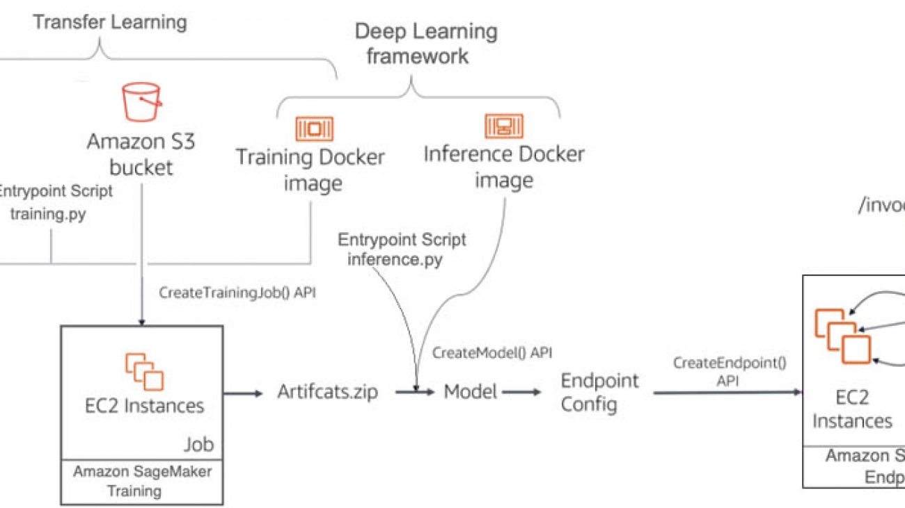
Rajarao Vijjapu is a data architect with AWS. He works with AWS customers and partners to provide guidance and technical assistance about Big Data, Analytics, AI/ML and Security projects, helping them improve the value of their solutions when using AWS.

Read More

AWS is excited to announce the winner of the second AWS DeepComposer Chartbusters challenge, Lena Taupier. AWS DeepComposer gives developers a creative way to get started with machine learning (ML). In June, we launched the Chartbusters challenge, a global competition where developers use AWS DeepComposer to create original compositions and compete to showcase their ML and generative AI skills. The second challenge, Spin the Model, required developers to bring their own data and create a custom genre model using a sample Amazon SageMaker notebook.

When Lena Taupier first attended the AWS DeepComposer workshop at re:Invent 2019, she had no idea she would be the winner of the Spin the Model challenge. Lena, a software developer for Blubrry, helps lead the company’s cloud infrastructure and applications development team. She also has her own blog in which she creates tutorials to make AWS skills more accessible. She describes herself as an ML novice and never would have thought she’d be experimenting with machine learning today.

We interviewed Lena about her experience competing in the second Chartbusters challenge, which ran from July 31 to August 23, and asked her to tell us more about how she created her winning composition.

Lena with her AWS DeepComposer keyboard

Getting started with machine learning

Lena has a background in classical piano, so when she first learned about AWS DeepComposer, she was intrigued to learn more.

“When I was younger, I studied classical piano pretty seriously and I still enjoy playing piano very much. I was at re:Invent last year when AWS DeepComposer was announced, and I was so excited by the thought of learning about AI while creating music. I ended up waiting in line for several hours to attend one of the demo sessions, but I was so eager to try it out that I didn’t even mind!”

Lena first heard about the AWS DeepComposer Chartbusters challenge through the AWS blog, and thought the challenge was a great way to get started with ML.

Building in AWS DeepComposer

To get started, Lena used the AWS DeepComposer learning capsules to learn more about AR-CNN models. The learning capsules provide easy-to-consume, bite-size content to help you learn the concepts of generative AI algorithms.

“The first thing I did was to go through the learning capsules about autoregressive convolutional neural networks and how to train AR-CNN models. It was a great resource for learning about different generative AI techniques.”

The Chartbusters Spin the Model challenge required developers to get creative and make a custom genre model by bringing their own dataset to train. Lena drew from her own background, having grown up in St. Lucia, a city with a history of oral and folk traditional music.

“Once I had a good understanding, I started brainstorming about what kind of music I wanted to use to train my model. I’m from St. Lucia, a small island in the Caribbean, where there is a rich history of unique music, so I thought it would be interesting to incorporate songs from there. I decided to create some of my own music clips inspired by Calypso and St. Lucian folk music to supplement my dataset.”

Lena’s workstation for the AWS DeepComposer Chartbusters challenge

Next, Lena began training her model using Amazon SageMaker.

“Once I had my dataset, I created a Jupyter notebook within Amazon SageMaker, using the repository provided as a starting point. I experimented with the hyperparameters and then let the training run overnight because I knew it would take many hours to process. The next day, I was finally able to use my trained model to make new music!”

Lena used her AWS DeepComposer keyboard and the music studio to generate different melodies and compositions until she was satisfied with her two final compositions.

“I submitted two AI-generated songs. The main theme in “Little Banjo” was inspired by a famous St. Lucian folk song. Layered on top of the melody generated by my AR-CNN model, I also used the MuseGAN Rock model to generate additional instruments for accompaniment. The other song is meant to resemble the style of Calypso, and has a rich beat with trumpet lines to complement the melody. I named it “Home Sweet Home” because I started feeling nostalgic about home after listening to so much St. Lucian music for this project!”

Lena working on her compositions in the AWS DeepComposer console

You can listen to Lena’s winning composition, “Home Sweet Home,” on the AWS DeepComposer SoundCloud page.

Conclusion

The AWS DeepComposer Chartbusters challenge Spin the Model helped Lena learn about generative AI through a hands-on and fun experience.

“By participating in this challenge, I was able to learn a lot about different generative AI techniques in a very hands-on way, which is the best way to learn. As someone with very little experience in AI and machine learning, it was a great feeling of accomplishment to be able to train a custom AR-CNN model and actually generate results.”

The Chartbusters challenge empowered Lena to go from beginner knowledge ML to creating winning compositions with AWS DeepComposer.

“I think AWS DeepComposer is such a great tool for reducing the barrier of entry into machine learning and making those concepts accessible to more people […] Even just a few months ago, I never would have thought I’d be experimenting with AI/ML. This challenge was such a great learning experience! I know there’s so much more to learn so I will definitely continue to explore and dive deeper.”

Her advice to future competitors? Now is the time to get started with ML.

“As a developer, I think it’s such an exciting time to have access to the cloud, because it really widens your horizons on what you can do […] The Chartbusters challenge is the perfect opportunity to get involved and start learning in a fun, creative, and hands-on manner!”

Congratulations to Lena for her well-deserved win!

We hope Lena’s story has inspired you to learn more about ML and get started with AWS DeepComposer. Check out the next AWS DeepComposer Chartbusters challenge, The Sounds of Science, running now until September 23.

About the Author

Paloma Pineda is a Product Marketing Manager for AWS Artificial Intelligence Devices. She is passionate about the intersection of technology, art, and human centered design. Out of the office, Paloma enjoys photography, watching foreign films, and cooking French cuisine.

Read More

Amazon Personalize is a machine learning (ML) service that enables you to personalize your website, app, ads, emails, and more with private, custom ML models that you can create with no prior ML experience. We’re excited to announce the general availability of Amazon Personalize in the EU (Frankfurt) Region. You can use Amazon Personalize to create higher-quality recommendations that respond to the specific needs, preferences, and changing behavior of your users, improving engagement and conversion. For more information, see Amazon Personalize Is Now Generally Available.

To use Amazon Personalize, you need to provide the service user interaction(events) data (such as page views, sign-ups, purchases etc.) from your applications, along with optional user demographic information (such as age, location) and a catalog of the items you want to recommend (such as articles, products, videos, or music). This data can be provided via Amazon S3 or be sent as a stream of user events via a JavaScript tracker or a server-side integration (learn more). Amazon Personalize then automatically processes and examines the data, identifies what is meaningful, and trains and optimizes a personalization model that is customized for your data. You can then easily invoke Amazon Personalize APIs from your business application and fetch personalized recommendations for your users.

Learn how our customers are using Amazon Personalize to improve product and content recommendations and for targeted marketing communications.

For more information about all the Regions Amazon Personalize is available in, see the AWS Region Table. Get started with Amazon Personalize by visiting the Amazon Personalize console and Developer Guide.

About the Author

Vaibhav Sethi is the Product Manager for Amazon Personalize. He focuses on delivering products that make it easier to build machine learning solutions. In his spare time, he enjoys hiking and reading.

Read More

Amazon SageMaker is a fully managed service that provides every developer and data scientist with the ability to build, train, and deploy machine learning (ML) models quickly. Amazon SageMaker removes the heavy lifting from each step of the ML process to make it easier to develop high-quality models. As datasets continue to increase in size, additional compute is required to reduce the amount of time it takes to train. One method to scale horizontally and add these additional resources on Amazon SageMaker is through the use of Horovod and Apache MXNet. In this post, we show how you can reduce training time with MXNet and Horovod on Amazon SageMaker. We also demonstrate how to further improve performance with advanced sections on Horovod autotuning, Horovod Timeline, Horovod Fusion, and MXNet optimization.

Distributed training

Distributed training of neural networks for computer vision (CV) and natural language processing (NLP) applications has become ubiquitous. With Apache MXNet, you only need to modify a few lines of code to enable distributed training.

Distributed training allows you to reduce training time by scaling horizontally. The goal is to split training tasks into independent subtasks and run these across multiple devices. There are primarily two approaches for training in parallel:

• Data parallelism – You distribute the data and share the model across multiple compute resources
• Model parallelism – You distribute the model and share transformed data across multiple compute resources.

In this post, we focus on data parallelism. Specifically, we discuss how Horovod and MXNet allow you to train efficiently on Amazon SageMaker.

Horovod overview

Horovod is an open-source distributed deep learning framework. It uses efficient inter-GPU and inter-node communication methods such as NVIDIA Collective Communications Library (NCCL) and Message Passing Interface (MPI) to distribute and aggregate model parameters between workers. Horovod makes distributed deep learning fast and easy by using a single-GPU training script and scaling it across many GPUs in parallel. It’s built on top of the ring-allreduce communication protocol. This approach allows each training process (such as a process running on a single GPU device) to talk to its peers and exchange gradients by averaging (called reduction) on a subset of gradients. The following diagram illustrates how ring-allreduce works.

Apache MXNet is integrated with Horovod through the distributed training APIs defined in Horovod, and you can convert the non-distributed training by following the higher level code skeleton, which we show in this post.

Although this greatly simplifies the process of using Horovod, you must consider other complexities. For example, you may need to install additional software and libraries to resolve your incompatibilities for making distributed training work. Horovod requires a certain version of Open MPI, and if you want to use high-performance training on NVIDIA GPUs, you need to install NCCL libraries. These complexities are amplified when you scale across multiple devices, because you need to make sure all the software and libraries in the new nodes are properly installed and configured. Amazon SageMaker includes all the required libraries to run distributed training with MXNet and Horovod. Prebuilt Amazon SageMaker Docker images come with popular open-source deep learning frameworks and pre-configured CUDA, cuDNN, MPI, and NCCL libraries. Amazon SageMaker manages the difficult process of properly installing and configuring your cluster. Amazon SageMaker and MXNet simplify training with Horovod by managing the complexities to support distributed training at scale.

Test problem and dataset

To benchmark the efficiencies realized by Horovod, we trained the notoriously resource-intensive model architectures Mask-RCNN and Faster-RCNN. These model architectures were first introduced in 2018 and 2016, respectively, and are currently considered the baseline model architectures for two popular CV tasks: instance segmentation (Mask-RCNN) and object detection (Faster-RCNN). Mask-RCNN builds upon Faster-RCNN by adding a mask for segmentation. Apache MXNet provides pre-built Mask-RCNN and Faster-RCNN models as part of the GluonCV model zoo, simplifying the process of training these models.

To train our object detection and instance segmentation models, we used the popular COCO2017 dataset. This dataset provides more than 200,000 images and their corresponding labels. The COCO2017 dataset is considered an industry standard for benchmarking CV models.

GluonCV is a CV toolkit built on top of MXNet. It provides out-of-the-box support for various CV tasks, including data loading and preprocessing for many common algorithms available within its model zoo. It also provides a tutorial on getting the COCO2017 dataset.

To make this process replicable for Amazon SageMaker users, we show an entire end-to-end process for training Mask-RCNN and Faster-RCNN with Horovod and MXNet. To begin, we first open the Jupyter environment in your Amazon SageMaker notebook and use the conda_mxnet_p36 kernel. Next, we install the required Python packages:

! pip install gluoncv
! pip install pycocotools

We use the GluonCV toolkit to download the COCO2017 dataset onto our Amazon SageMaker notebook:

import gluoncv as gcv
gcv.utils.download('https://gluon-cv.mxnet.io/_downloads/b6ade342998e03f5eaa0f129ad5eee80/mscoco.py',path='./')
#Now to install the dataset. Warning, this may take a while
! python mscoco.py --download-dir data

We upload COCO2017 to the specified Amazon Simple Storage Service (Amazon S3) bucket using the following command:

! aws s3 cp './data/' s3://<INSERT BUCKET NAME>/ --recursive –quiet

Training script with Horovod Support

To use Horovod in your training script, you only need to make a few modifications. For code samples and instructions, see Horovod with MXNet. In addition, many GluonCV models in the model zoo have scripts that already support Horovod out of the box. In this section, we review the key changes required for Horovod to correctly work on Amazon SageMaker with Apache MXNet. The following code follows directly from the Horovod documentation:

import mxnet as mx
import horovod.mxnet as hvd
from mxnet import autograd

# Initialize Horovod, this has to be done first as it activates Horovod.
hvd.init()

# GPU setup 
context =[mx.gpu(hvd.local_rank())] #local_rank is the specific gpu on that 
# instance
num_gpus = hvd.size() #This is how many total GPUs you will be using.

#Typically, in your data loader you will want to shard your dataset. For 
# example, in the train_mask_rcnn.py script 
train_sampler = 
        gcv.nn.sampler.SplitSortedBucketSampler(...,
                                                num_parts=hvd.size() if args.horovod else 1,
                                                part_index=hvd.rank() if args.horovod else 0)

#Normally, we would shard the dataset first for Horovod.
val_loader = mx.gluon.data.DataLoader(dataset, len(ctx), ...) #... is for your # other arguments

    
# You build and initialize your model as usual.
model = ...

# Fetch and broadcast the parameters.
params = model.collect_params()
if params is not None:
    hvd.broadcast_parameters(params, root_rank=0)

# Create DistributedTrainer, a subclass of gluon.Trainer.
trainer = hvd.DistributedTrainer(params, opt)

# Create loss function and train your model as usual. 

Training job configuration

The Amazon SageMaker MXNet estimator class supports Horovod via the distributions parameter. We need to add a predefined mpi parameter with the enabled flag, and define the following additional parameters:

• processes_per_host (int) – Number of processes MPI should launch on each host. This parameter is usually equal to the number of GPU devices available on any given instance.
• custom_mpi_options (str) – Any custom mpirun flags passed in this field are added to the mpirun command and run by Amazon SageMaker for Horovod training.

The follow example code initializes the distributions parameters:

distributions = {'mpi': {
                    'enabled': True,
                    'processes_per_host': 8, #Each instance has 8 gpus
			'custom_mpi_options': '-verbose --NCCL_DEBUG=INFO'
                        }
                }

Next, we need to configure other parameters of our training job, such as hyperparameters, and the input and output Amazon S3 locations. To do this, we use the MXNet estimator class from the Amazon SageMaker Python SDK:

#Define the basic configuration of your Horovod-enabled Sagemaker training 
# cluster.
num_instances = 2 # How many nodes you want to use.
instance_family = 'ml.p3dn.24xlarge' # Which instance type you want to use.


estimator = MXNet(
                entry_point=<source_name>.py,         #Script entry point.
                source_dir='./source',                #Script Location
                role=role, 
                train_instance_type=instance_family,
                train_instance_count=num_instances,
                framework_version='1.6.0',            #MXNet version.
                train_volume_size=100,                #Size for the dataset.
                py_version='py3',                     #Python version.
                hyperparameters=hyperparameters,
                distributions=distributions           #For use with Horovod.

We’re now ready to start our first Horovod-powered training job with the following command:

            estimator.fit(
                {'data':'s3://' + bucket_name + '/data'}
            )

Results

We performed these benchmarks on two similar GPU instance types: the p3.16xlarge and the more powerful p3dn.24xlarge. Although both have 8 NVIDIA V100 GPUs, the latter instance is designed with distributed training in mind. In addition to a high-throughput network interface amenable to the inter-node data transfers inherent in distributed training, the p3dn.24xlarge boasts more compute and additional memory over the p3.16xlarge.

We ran benchmarks in three different use cases. In the first and second use cases, we trained the models on a single instance using all 8 local GPUs, to demonstrate the efficiencies gained by using Horovod to manage local training across multiple GPUs. In the third use case, we used Horovod for distributed training across multiple instances, each with 8 local GPUs, to demonstrate the additional efficiency increase by scaling horizontally.

The following table summarizes the time and accuracy for each training scenario.

As expected, when using Horovod to distribute training across multiple instances, the time to convergence is significantly reduced. Additionally, even when training on a single instance, Horovod substantially increases training efficiency when using multiple local GPUs, as compared to the default parameter-server approach. Horovod’s simplified APIs and abstractions enable you to unlock efficiency gains when training across multiple GPUs, both on a single machine or many. For more information about using this approach for scaling batch size and learning rate, see Accurate, Large Minibatch SGD: Training ImageNet in 1 Hour.

With the improvement in training time enabled by Horovod and Amazon SageMaker, you can focus more on improving your algorithms instead of waiting for jobs to finish training. You can train in parallel across multiple instances with marginal impact to mean Average Precision (mAP).

Optimizing Horovod training

Horovod provides several additional utilities that allow you to analyze and optimize training performance.

Horovod autotuning

Finding the optimal combinations of parameters for a given combination of model and cluster size may require several iterations of trial and error.

The autotune feature allows you to automate this trial-and-error activity within a single training job, and uses Bayesian optimization to search through the parameter space for the most performant combination of parameters. Horovod searches for the best combination of parameters in the first cycles of a training job. When it defines the best combination, Horovod writes it in the autotune log and uses this combination for the remainder of the training job. For more information, see Autotune: Automated Performance Tuning.

To enable autotuning and capture the search log, pass the following parameters in your MPI configuration:

{
    'mpi':
    {
        'enabled': True,
        'custom_mpi_options': '-x HOROVOD_AUTOTUNE=1 -x         HOROVOD_AUTOTUNE_LOG=/opt/ml/output/autotune_log.csv'
    }
}

Horovod Timeline

Horovod Timeline is a report available after training completion that captures all activities in the Horovod ring. This is useful to understand which operations are taking the longest and identify optimization opportunities. For more information, see Analyze Performance.

To generate a timeline file, add the following parameters in your MPI command:

{
    'mpi':
    {
        'enabled': True,
        'custom_mpi_options': '-x HOROVOD_TIMELINE=/opt/ml/output/timeline.json'
    }
}

The /opt/ml/output is a directory with a specific purpose. After the training job is complete, Amazon SageMaker automatically archives all files in this directory and uploads it to an Amazon S3 location that you define in the Python Amazon SageMaker SDK API.

Tensor Fusion

The Tensor Fusion feature allows you to perform batch allreduce operations at training time. This typically results in better overall performance. For more information, see Tensor Fusion. By default, Tensor Fusion is enabled and has a buffer size of 64 MB. You can modify buffer size using a custom MPI flag as follows (for our use case, we override the default 64 MB buffer value with 32 MB):

{
    'mpi':
    {
        'enabled': True,
        'custom_mpi_options': '-x HOROVOD_FUSION_THRESHOLD=33554432'
    }
}

You can also adjust batch cycles using the HOROVOD_CYCLE_TIME parameter. Cycle time is defined in milliseconds. See the following code:

{
    'mpi':
    {
        'enabled': True,
        'custom_mpi_options': '-x HOROVOD_CYCLE_TIME=5'
    }
}

Optimizing MXNet models

Another optimization technique is related to optimizing the MXNet model itself. We recommend running the code with os.environ['MXNET_CUDNN_AUTOTUNE_DEFAULT'] = '1'. Then you can copy the best OS environment variables for future training. In our testing, we found the following to be the best results:

os.environ['MXNET_GPU_MEM_POOL_TYPE'] = 'Round'
os.environ['MXNET_GPU_MEM_POOL_ROUND_LINEAR_CUTOFF'] = '26'
os.environ['MXNET_EXEC_BULK_EXEC_MAX_NODE_TRAIN_FWD'] = '999'
os.environ['MXNET_EXEC_BULK_EXEC_MAX_NODE_TRAIN_BWD'] = '25'
os.environ['MXNET_GPU_COPY_NTHREADS'] = '1'
os.environ['MXNET_OPTIMIZER_AGGREGATION_SIZE'] = '54'

Conclusion

In this post, we demonstrated how to reduce training time with Horovod and Apache MXNet on Amazon SageMaker. You can train your model out of the box without worrying about any additional complexities.

For more information about deep learning and MXNet, see the MXNet crash course and Dive into Deep Learning book. You can also get started on the MXNet website and MXNet GitHub examples directory. If you’re new to distributed training and want to dive deeper, we highly recommend reading the paper Horovod: fast and easy distributed deep learning in TensorFlow. If you use the AWS Deep Learning Containers and AWS Deep Learning AMIs, you can learn how to set up this workflow in that environment in our recent post How to run distributed training using Horovod and MXNet on AWS DL containers and AWS Deep Learning AMIs.

About the Authors

Vadim Dabravolski is AI/ML Solutions Architect with FinServe team. He is focused on Computer Vision and NLP technologies and how to apply them to business use cases. After hours Vadim enjoys jogging in NYC boroughs, reading non-fiction (business, history, culture, politics, you name it), and rarely just doing nothing.

Corey Barrett is a Data Scientist in the Amazon ML Solutions Lab. As a member of the ML Solutions Lab, he leverages Machine Learning and Deep Learning to solve critical business problems for AWS customers. Outside of work, you can find him enjoying the outdoors, sipping on scotch, and spending time with his family.

Chaitanya Bapat is a Software Engineer with the AWS Deep Learning team. He works on Apache MXNet and integrating the framework with Amazon Sagemaker, DLC and DLAMI. In his spare time, he loves watching sports and enjoys reading books and learning Spanish.

Karan Jariwala is a Software Development Engineer on the AWS Deep Learning team. His work focuses on training deep neural networks. Outside of work, he enjoys hiking, swimming, and playing tennis.

Read More