When ingesting data into Amazon OpenSearch, customers often need to augment data before putting it into their indexes. For instance, you might be ingesting log files with an IP address and want to get a geographic location for the IP address, or you might be ingesting customer comments and want to identify the language they are in. Traditionally, this requires an external process that complicates data ingest pipelines and can cause a pipeline to fail. OpenSearch offers a wide range of third-party machine learning (ML) connectors to support this augmentation.

This post highlights two of these third-party ML connectors. The first connector we demonstrate is the Amazon Comprehend connector. In this post, we show you how to use this connector to invoke the LangDetect API to detect the languages of ingested documents.

The second connector we demonstrate is the Amazon Bedrock connector to invoke the Amazon Titan Text Embeddings v2 model so that you can create embeddings from ingested documents and perform semantic search.

Solution overview

We use Amazon OpenSearch with Amazon Comprehend to demonstrate the language detection feature. To help you replicate this setup, we’ve provided the necessary source code, an Amazon SageMaker notebook, and an AWS CloudFormation template. You can find these resources in the sample-opensearch-ml-rest-api GitHub repo.

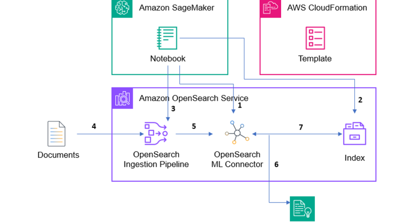
The reference architecture shown in the preceding figure shows the components used in this solution. A SageMaker notebook is used as a convenient way to execute the code that is provided in the Github repository provided above.

Prerequisites

To run the full demo using the sample-opensearch-ml-rest-api, make sure you have an AWS account with access to:

• Run a CloudFormation template
• Create AWS Identity and Access Management (IAM) roles and policies
• Create a SageMaker notebook
• Create an Amazon OpenSearch cluster
• Create an Amazon Simple Storage Service (Amazon S3) bucket
• Invoke Amazon Comprehend APIs
• Invoke Amazon Bedrock models (for part 2)

Part 1: The Amazon Comprehend ML connector

Set up OpenSearch to access Amazon Comprehend

Before you can use Amazon Comprehend, you need to make sure that OpenSearch can call Amazon Comprehend. You do this by supplying OpenSearch with an IAM role that has access to invoke the DetectDominantLanguage API. This requires the OpenSearch Cluster to have fine grained access control enabled. The CloudFormation template creates a role for this called <Your Region>-<Your Account Id>-SageMaker-OpenSearch-demo-role. Use the following steps to attach this role to the OpenSearch cluster.

1. Open the OpenSearch Dashboard console—you can find the URL in the output of the CloudFormation template—and sign in using the username and password you provided.

2. Choose Security in the left-hand menu (if you don’t see the menu, choose the three horizontal lines icon at the top left of the dashboard).
3. From the security menu, select Roles to manage the OpenSearch roles.
4. In the search box. enter ml_full_access role.
5. Select the Mapped users link to map the IAM role to this OpenSearch role.
6. On the Mapped users screen, choose Manage mapping to edit the current mappings.
7. Add the IAM role mentioned previously to map it to the ml_full_access role, this will allow OpenSearch to access the needed AWS resources from the ml-commons plugin. Enter your IAM role Amazon Resource Name (ARN) (arn:aws:iam::<your account id>:role/<your region>-<your account id>-SageMaker-OpenSearch-demo-role) in the backend roles field and choose Map.

Set up the OpenSearch ML connector to Amazon Comprehend

In this step, you set up the ML connector to connect Amazon Comprehend to OpenSearch.

1. Get an authorization token to use when making the call to OpenSearch from the SageMaker notebook. The token uses an IAM role attached to the notebook by the CloudFormation template that has permissions to call OpenSearch. That same role is mapped to the OpenSearch admin role in the same way you just mapped the role to access Amazon Comprehend. Use the following code to set this up:

awsauth = AWS4Auth(credentials.access_key,
credentials.secret_key,
region,
'es',
session_token=credentials.token)

2. Create the connector. It needs a few pieces of information:
   1. It needs a protocol. For this example, use aws_sigv4, which allows OpenSearch to use an IAM role to call Amazon Comprehend.
   2. Provide the ARN for this role, which is the same role you used to set up permissions for the ml_full_access role.
   3. Provide comprehend as the service_name, and DetectDominateLanguage as the api_name.
   4. Provide the URL to Amazon Comprehend and set up how to call the API and what data to pass to it.

The final call looks like:

comprehend = boto3.client('comprehend', region_name='us-east-1')
path = '/_plugins/_ml/connectors/_create'
url = host + path

payload = {
  "name": "Comprehend lang identification",
  "description": "comprehend model",
  "version": 1,
  "protocol": "aws_sigv4",
  "credential": {
    "roleArn": sageMakerOpenSearchRoleArn
  },
  "parameters": {
    "region": "us-east-1",
    "service_name": "comprehend",
    "api_version": "20171127",
    "api_name": "DetectDominantLanguage",
    "api": "Comprehend_${parameters.api_version}.${parameters.api_name}",
    "response_filter": "$"
  },
  "actions": [
    {
      "action_type": "predict",
      "method": "POST",
      "url": "https://${parameters.service_name}.${parameters.region}.amazonaws.com",
      "headers": {
        "content-type": "application/x-amz-json-1.1",
        "X-Amz-Target": "${parameters.api}"
      },
      "request_body": "{"Text": "${parameters.Text}"}" 
    }
  ]
}

comprehend_connector_response = requests.post(url, auth=awsauth, json=payload)
comprehend_connector = comprehend_connector_response.json()["connector_id"]

Register the Amazon Comprehend API connector

The next step is to register the Amazon Comprehend API connector with OpenSearch using the Register Model API from OpenSearch.

• Use the comprehend_connector that you saved from the last step.

path = '/_plugins/_ml/models/_register'
url = host + path

payload = {
    "name": "comprehend lang id API",
    "function_name": "remote",
    "description": "API to detect the language of text",
    "connector_id": comprehend_connector
}
headers = {"Content-Type": "application/json"}

response = requests.post(url, auth=awsauth, json=payload, headers=headers)
comprehend_model_id = response.json()['model_id']

As of OpenSearch 2.13, when the model is first invoked, it’s automatically deployed. Prior to 2.13 you would have to manually deploy the model within OpenSearch.

Test the Amazon Comprehend API in OpenSearch

With the connector in place, you need to test the API to make sure it was set up and configured correctly.

1. Make the following call to OpenSearch.

path = '/_plugins/_ml/models/'+ comprehend_model_id + '/_predict'
url = host + path

headers = {"Content-Type": "application/json"}
payload = {
    "parameters": {
        "Text": "你知道厕所在哪里吗"
    }
}

response = requests.post(url, auth=awsauth, json=payload, headers=headers)
print(response.json())

2. You should get the following result from the call, showing the language code as zh with a score of 1.0:

{
   "inference_results":[
      {
         "output":[
            {
               "name":"response",
               "dataAsMap":{
                  "response":{
                     "Languages":[
                        {
                           "LanguageCode":"zh",
                           "Score":1.0
                        }
                     ]
                  }
               }
            }
         ],
         "status_code":200
      }
   ]
}

Create an ingest pipeline that uses the Amazon Comprehend API to annotate the language

The next step is to create a pipeline in OpenSearch that calls the Amazon Comprehend API and adds the results of the call to the document being indexed. To do this, you provide both an input_map and an output_map. You use these to tell OpenSearch what to send to the API and how to handle what comes back from the call.

path = '/_ingest/pipeline/comprehend_language_identification_pipeline'
url = host + path

payload = {
  "description": "ingest identify lang with the comprehend API",
  "processors":[
    {
      "ml_inference": {
        "model_id": comprehend_model_id,
        "input_map": [
            {
               "Text": "Text"
            }
        ],
        "output_map": [
            {  
               "detected_language": "response.Languages[0].LanguageCode",
               "language_score": "response.Languages[0].Score"
            }
        ]
      }
    }
  ]
}
headers = {"Content-Type": "application/json"}
response = requests.put(url, auth=awsauth, json=payload, headers=headers)

You can see from the preceding code that you are pulling back both the top language result and its score from Amazon Comprehend and adding those fields to the document.

Part 2: The Amazon Bedrock ML connector

In this section, you use Amazon OpenSearch with Amazon Bedrock through the ml-commons plugin to perform a multilingual semantic search. Make sure that you have the solution prerequisites in place before attempting this section.

In the SageMaker instance that was deployed for you, you can see the following files: english.json, french.json, german.json.

These documents have sentences in their respective languages that talk about the term spring in different contexts. These contexts include spring as a verb meaning to move suddenly, as a noun meaning the season of spring, and finally spring as a noun meaning a mechanical part. In this section, you deploy Amazon Titan Text Embeddings model v2 using the ml connector for Amazon Bedrock. You then use this embeddings model to create vectors of text in three languages by ingesting the different language JSON files. Finally, these vectors are stored in Amazon OpenSearch to enable semantic searches to be used across the language sets.

Amazon Bedrock provides streamlined access to various powerful AI foundation models through a single API interface. This managed service includes models from Amazon and other leading AI companies. You can test different models to find the ideal match for your specific needs, while maintaining security, privacy, and responsible AI practices. The service enables you to customize these models with your own data through methods such as fine-tuning and Retrieval Augmented Generation (RAG). Additionally, you can use Amazon Bedrock to create AI agents that can interact with enterprise systems and data, making it a comprehensive solution for developing generative AI applications.

The reference architecture in the preceding figure shows the components used in this solution.

(1) First we must create the OpenSearch ML connector via running code within the Amazon SageMaker notebook. The connector essentially creates a Rest API call to any model, we specifically want to create a connector to call the Titan Embeddings model within Amazon Bedrock.

(2) Next, we must create an index to later index our language documents into. When creating an index, you can specify its mappings, settings, and aliases.

(3) After creating an index within Amazon OpenSearch, we want to create an OpenSearch Ingestion pipeline that will allow us to streamline data processing and preparation for indexing, making it easier to manage and utilize the data. (4) Now that we have created an index and set up a pipeline, we can start indexing our documents into the pipeline.

(5 – 6) We use the pipeline in OpenSearch that calls the Titan Embeddings model API. We send our language documents to the titan embeddings model, and the model returns vector embeddings of the sentences.

(7) We store the vector embeddings within our index and perform vector semantic search.

While this post highlights only specific areas of the overall solution, the SageMaker notebook has the code and instructions to run the full demo yourself.

Before you can use Amazon Bedrock, you need to make sure that OpenSearch can call Amazon Bedrock. .

Load sentences from the JSON documents into dataframes

Start by loading the JSON document sentences into dataframes for more structured organization. Each row can contain the text, embeddings, and additional contextual information:

import json
import pandas as pd

def load_sentences(file_name):
    sentences = []
    with open(file_name, 'r', encoding='utf-8') as file:
        for line in file:
            try:
                data = json.loads(line)
                if 'sentence' in data and 'sentence_english' in data:
                    sentences.append({
                        'sentence': data['sentence'],
                        'sentence_english': data['sentence_english']
                    })
            except json.JSONDecodeError:
                # Skip lines that are not valid JSON (like the index lines)
                continue
    
    return pd.DataFrame(sentences)

# Usage
german_df = load_sentences('german.json')
english_df = load_sentences('english.json')
french_df = load_sentences('french.json')
# print(french_df.head())

Create the OpenSearch ML connector to Amazon Bedrock

After loading the JSON documents into dataframes, you’re ready to set up the OpenSearch ML connector to connect Amazon Bedrock to OpenSearch.

1. The connector needs the following information.
   1. It needs a protocol. For this solution, use aws_sigv4, which allows OpenSearch to use an IAM role to call Amazon Bedrock.
   2. Provide the same role used earlier to set up permissions for the ml_full_access role.
   3. Provide the service_name, model, dimensions of the model, and embedding type.

The final call looks like the following:

payload = {
  "name": "Amazon Bedrock Connector: embedding",
  "description": "The connector to bedrock Titan embedding model",
  "version": 1,
  "protocol": "aws_sigv4",
  "parameters": {
    "region": "us-east-1",
    "service_name": "bedrock",
    "model": "amazon.titan-embed-text-v2:0",
    "dimensions": 1024,
    "normalize": True,
    "embeddingTypes": ["float"]
  },
  "credential": {
    "roleArn": sageMakerOpenSearchRoleArn
  },
  "actions": [
    {
      "action_type": "predict",
      "method": "POST",
      "url": "https://bedrock-runtime.${parameters.region}.amazonaws.com/model/${parameters.model}/invoke",
      "headers": {
        "content-type": "application/json",
        "x-amz-content-sha256": "required"
      },
      "request_body": "{ "inputText": "${parameters.inputText}", "dimensions": ${parameters.dimensions}, "normalize": ${parameters.normalize}, "embeddingTypes": ${parameters.embeddingTypes} }",
      "pre_process_function": "connector.pre_process.bedrock.embedding",
      "post_process_function": "connector.post_process.bedrock.embedding"
    }
  ]
}

bedrock_connector_response = requests.post(url, auth=awsauth, json=payload, headers=headers)

bedrock_connector_3 = bedrock_connector_response.json()["connector_id"]
print('Connector id: ' + bedrock_connector_3)

Test the Amazon Titan Embeddings model in OpenSearch

After registering and deploying the Amazon Titan Embeddings model using the Amazon Bedrock connector, you can test the API to verify that it was set up and configured correctly. To do this, make the following call to OpenSearch:

headers = {"Content-Type": "application/json"}
payload = {
  "parameters": {
    "inputText": "It's nice to see the flowers bloom and hear the birds sing in the spring"
  }
}
response = requests.post(url, auth=awsauth, json=payload, headers=headers)
print(response.json())

You should get a formatted result, similar to the following, from the call that shows the generated embedding from the Amazon Titan Embeddings model:

{'inference_results': [{'output': [{'name': 'sentence_embedding', 'data_type': 'FLOAT32', 'shape': [1024], 'data': [-0.04092199727892876, 0.052057236433029175, -0.03354490175843239, 0.04398418962955475, -0.001235315459780395, -0.03284895047545433, -0.014197427779436111, 0.0098129278048…

The preceding result is significantly shortened compared to the actual embedding result you might receive. The purpose of this snippet is to show you the format.

Create the index pipeline that uses the Amazon Titan Embeddings model

Create a pipeline in OpenSearch. You use this pipeline to tell OpenSearch to send the fields you want embeddings for to the embeddings model.

pipeline_name = "titan_embedding_pipeline_v2"
url = f"{host}/_ingest/pipeline/{pipeline_name}"

pipeline_body = {
    "description": "Titan embedding pipeline",
    "processors": [
        {
            "text_embedding": {
                "model_id": bedrock_model_id,
                "field_map": {
                    "sentence": "sentence_vector"
                }
            }
        }
    ]
}

response = requests.put(url, auth=awsauth, json=pipeline_body, headers={"Content-Type": "application/json"})
print(response.text)

Create an index

With the pipeline in place, the next step is to create an index that will use the pipeline. There are three fields in the index:

• sentence_vector – This is where the vector embedding will be stored when returned from Amazon Bedrock.
• sentence – This is the non-English language sentence.
• sentence_english – this is the English translation of the sentence. Include this to see how well the model is translating the original sentence.

index_name = 'bedrock-knn-index-v2'
url = f'{host}/{index_name}'
mapping = {
    "mappings": {
        "properties": {
            "sentence_vector": {
                "type": "knn_vector",
                "dimension": 1024,  
                "method": {
                    "name": "hnsw",
                    "space_type": "l2",
                    "engine": "nmslib"
                },
                "store":True
            },
            "sentence":{
                "type": "text",
                "store": True
            },
            "sentence_english":{
                "type": "text",
                "store": True
            }
        }
    },
    "settings": {
        "index": {
            "knn": True,
            "knn.space_type": "cosinesimil",
            "default_pipeline": pipeline_name
        }
    }
}

response = requests.put(url, auth=awsauth, json=mapping, headers={"Content-Type": "application/json"})
print(f"Index creation response: {response.text}")

Load dataframes into the index

Earlier in this section, you loaded the sentences from the JSON documents into dataframes. Now, you can index the documents and generate embeddings for them using the Amazon Titan Text Embeddings Model v2. The embeddings will be stored in the sentence_vector field.

index_name = "bedrock-knn-index-v2"

def index_documents(df, batch_size=100):
    total = len(df)
    for start in range(0, total, batch_size):
        end = min(start + batch_size, total)
        batch = df.iloc[start:end]

        bulk_data = []
        for _, row in batch.iterrows():
            # Prepare the action metadata
            action = {
                "index": {
                    "_index": index_name
                }
            }
            # Prepare the document data
            doc = {
                "sentence": row['sentence'],
                "sentence_english": row['sentence_english']
            }
            
            # Add the action and document to the bulk data
            bulk_data.append(json.dumps(action))
            bulk_data.append(json.dumps(doc))

        # Join the bulk data with newlines
        bulk_body = "n".join(bulk_data) + "n"

        # Send the bulk request
        bulk_url = f"{host}/_bulk"
        response = requests.post(bulk_url, auth=awsauth, data=bulk_body, headers={"Content-Type": "application/x-ndjson"})

        if response.status_code == 200:
            print(f"Successfully indexed batch {start}-{end} of {total}")
        else:
            print(f"Error indexing batch {start}-{end} of {total}: {response.text}")

        # Optional: add a small delay to avoid overwhelming the cluster
        time.sleep(1)

# Index your documents
print("Indexing German documents:")
index_documents(german_df)
print("nIndexing English documents:")
index_documents(english_df)
print("nIndexing French documents:")
index_documents(french_df)

Perform semantic k-NN across the documents

The final step is to perform a k-nearest neighbor (k-NN) search across the documents.

# Define your OpenSearch host and index name
index_name = "bedrock-knn-index-v2"
def semantic_search(query_text, k=5):
    search_url = f"{host}/{index_name}/_search"
    # First, index the query to generate its embedding
    index_doc = {
        "sentence": query_text,
        "sentence_english": query_text  # Assuming the query is in English
    }
    index_url = f"{host}/{index_name}/_doc"
    index_response = requests.post(index_url, auth=awsauth, json=index_doc, headers={"Content-Type": "application/json"})
    
    if index_response.status_code != 201:
        print(f"Failed to index query document: {index_response.text}")
        return []
    
    # Retrieve the indexed query document to get its vector
    doc_id = index_response.json()['_id']
    get_url = f"{host}/{index_name}/_doc/{doc_id}"
    get_response = requests.get(get_url, auth=awsauth)
    query_vector = get_response.json()['_source']['sentence_vector']
    
    # Now perform the KNN search
    search_query = {
        "size": 30,
        "query": {
            "knn": {
                "sentence_vector": {
                    "vector": query_vector,
                    "k": 30
                }
            }
        },
        "_source": ["sentence", "sentence_english"]
    }

    search_response = requests.post(search_url, auth=awsauth, json=search_query, headers={"Content-Type": "application/json"})
    
    if search_response.status_code != 200:
        print(f"Search failed with status code {search_response.status_code}")
        print(search_response.text)
        return []

    # Clean up - delete the temporary query document
    delete_url = f"{host}/{index_name}/_doc/{doc_id}"
    requests.delete(delete_url, auth=awsauth)

    return search_response.json()['hits']['hits']

# Example usage
query = "le soleil brille"
results = semantic_search(query)

if results:
    print(f"Search results for: '{query}'")
    for result in results:
        print(f"Score: {result['_score']}")
        print(f"Sentence: {result['_source']['sentence']}")
        print(f"English: {result['_source']['sentence_english']}")
        print()
else:
    print("No results found or search failed.")

The example query is in French and can be translated to the sun is shining. Keeping in mind that the JSON documents have sentences that use spring in different contexts, you’re looking for query results and vector matches of sentences that use spring in the context of the season of spring.

Here are some of the results from this query:

Search results for: ' le soleil brille'
Score: 0.40515712
Sentence: Les premiers rayons de soleil au printemps réchauffent la terre.
English: The first rays of spring sunshine warm the earth.

Score: 0.40117615
Sentence: Die ersten warmen Sonnenstrahlen kitzeln auf der Haut im Frühling.
English: The first warm sun rays tickle the skin in spring.

Score: 0.3999985
Sentence: Die ersten Sonnenstrahlen im Frühling wecken die Lebensgeister.
English: The first rays of sunshine in spring awaken the spirits.

This shows that the model can provide results across all three languages. It is important to note that the confidence scores for these results might be low because you’ve only ingested a couple documents with a handful of sentences in each for this demo. To increase confidence scores and accuracy, ingest a robust dataset with multiple languages and plenty of sentences for reference.

Clean Up

To avoid incurring future charges, go to the AWS Management Console for CloudFormation console and delete the stack you deployed. This will terminate the resources used in this solution.

Benefits of using the ML connector for machine learning model integration with OpenSearch

There are many ways you can perform k-nn semantic vector searches; a popular methods is to deploy external Hugging Face sentence transformer models to a SageMaker endpoint. The following are the benefits of using the ML connector approach we showed in this post, and why should you use it instead of deploying models to a SageMaker endpoint:

• Simplified architecture
  • Single system to manage
  • Native OpenSearch integration
  • Simpler deployment
  • Unified monitoring

• Operational benefits
  • Less infrastructure to maintain
  • Built-in scaling with OpenSearch
  • Simplified security model
  • Straightforward updates and maintenance

• Cost efficiency
  • Single system costs
  • Pay-per-use Amazon Bedrock pricing
  • No endpoint management costs
  • Simplified billing

Conclusion

Now that you’ve seen how you can use the OpenSearch ML connector to augment your data with external REST calls, we recommend that you visit the GitHub repo if you haven’t already and walk through the full demo yourselves. The full demo shows how you can use Amazon Comprehend for language detection and how to use Amazon Bedrock for multilingual semantic vector search, using the ml-connector plugin for both use cases. It also has sample text and JSON documents to ingest so you can see how the pipeline works.

About the Authors

John Trollinger is a Principal Solutions Architect supporting the World Wide Public Sector with a focus on OpenSearch and Data Analytics. John has been working with public sector customers over the past 25 years helping them deliver mission capabilities. Outside of work, John likes to collect AWS certifications and compete in triathlons.

Shwetha Radhakrishnan is a Solutions Architect for Amazon Web Services (AWS) with a focus in Data Analytics & Machine Learning. She has been building solutions that drive cloud adoption and help empower organizations to make data-driven decisions within the public sector. Outside of work, she loves dancing, spending time with friends and family, and traveling.

Read More

In the landscape of generative AI, organizations are increasingly adopting a structured approach to deploy their AI applications, mirroring traditional software development practices. This approach typically involves separate development and production environments, each with its own AWS account, to create logical separation, enhance security, and streamline workflows.

Amazon Bedrock is a fully managed service that offers a choice of high-performing foundation models (FMs) from leading AI companies such as AI21 Labs, Anthropic, Cohere, Meta, Mistral AI, Stability AI, and Amazon through a single API, along with a broad set of capabilities you need to build generative AI applications with security, privacy, and responsible AI. As organizations scale their AI initiatives, they often face challenges in efficiently managing and deploying custom models across different stages of development and across geographical regions.

To address these challenges, Amazon Bedrock introduces two key features: Model Share and Model Copy. These features are designed to streamline the AI development lifecycle, from initial experimentation to global production deployment. They enable seamless collaboration between development and production teams, facilitate efficient resource utilization, and help organizations maintain control and security throughout the customized model lifecycle.

In this comprehensive blog post, we’ll dive deep into the Model Share and Model Copy features, exploring their functionalities, benefits, and practical applications in a typical development-to-production scenario.

Prerequisites for Model Copy and Model Share

Before you can start using Model Copy and Model Share, the following prerequisites must be fulfilled:

1. AWS Organizations setup: Both the source account (the account sharing the model) and the target account (the account receiving the model) must be part of the same organization. You’ll need to create an organization if you don’t have one already, enable resource sharing, and invite the relevant accounts.
2. IAM permissions: 
   • For Model Share: Set up AWS Identity and Access Management (IAM) permissions for the sharing account to allow sharing using AWS Resource Access Manager (AWS RAM).
   • For Model Copy: Configure IAM permissions in both source and target AWS Regions to allow copying operations.
   • Attach the necessary IAM policies to the roles in both accounts to enable model sharing.
3. KMS key policies (Optional): If your models are encrypted with a customer-managed KMS key, you’ll need to set up key policies to allow the target account to decrypt the shared model or to encrypt the copied model with a specific KMS key.
4. Network configuration: Make sure that the necessary network configurations are in place, especially if you’re using VPC endpoints or have specific network security requirements.
5. Service quotas: Check and, if necessary, request increases for the number of custom models per account service quotas in both the source and target Regions and accounts.
6. Provisioned throughput support: Verify that the target Region supports provisioned throughput for the model you intend to copy. This is crucial because the copy job will be rejected if provisioned throughput isn’t supported in the target Region.

Model Share: Streamlining development-to-production workflows

The following figure shows the architecture of Model Share and Model Copy. It consists of a source account where the model is fined tuned. Next, Amazon Bedrock shares it with the recipient account which accepts the shared model in AWS Resource Access Manager (RAM). Then, the shared model can be copied to the desired AWS Region.

When managing Amazon Bedrock custom models in a development-to-production pipeline, it’s essential to securely share these models across different AWS accounts to streamline the promotion process to higher environments. The Amazon Bedrock Model Share feature addresses this need, enabling smooth sharing between development and production environments. Model Share enables the sharing of custom models fine-tuned on Amazon Bedrock between different AWS accounts within the same Region and organization. This feature is particularly useful for organizations that maintain separate development and production environments.

Important considerations: 

• Both the source and target AWS accounts must be in the same organization.
• Only models that have been fine-tuned within Amazon Bedrock can be shared.
• Base models and custom models imported using the custom model import (CMI) cannot be shared directly. For these, use the standard model import process in each AWS account.
• When sharing encrypted models, use a customer-managed KMS key and attach a key policy that allows the recipient account to decrypt the shared model. Specify the recipient account in the Principal field of the key policy.

Key benefits: 

• Simplified development-to-production transitions: Quickly move fine-tuned models on Amazon Bedrock from development to production environments.
• Enhanced team collaboration: Share models across different departments or project teams.
• Resource optimization: Reduce duplicate model customization efforts across your organization.

How it works: 

1. After a model has been fine-tuned in the source AWS account using Amazon Bedrock, the source AWS account can use the AWS Management Console for Amazon Bedrock to share the model.
2. The target AWS account accepts the shared model in AWS RAM.
3. The shared model in the target AWS account needs to be copied to the desired Regions.
4. After copying, the target AWS account can purchase provisioned throughput and use the model.
5. If using KMS encryption, make sure the key policy is properly set up for the recipient account.

Model Copy: Optimizing model deployment across Regions

The Amazon Bedrock Model Copy feature enables you to replicate custom models across different Regions within your account. This capability serves two primary purposes: it can be used independently for single-account deployments, or it can complement Model Share in multi-account scenarios, where you first share the model across accounts and then copy it. The feature is particularly valuable for organizations that require global model deployment, Regional load balancing, and robust disaster recovery solutions. By allowing flexible model distribution across Regions, Model Copy helps optimize your AI infrastructure for both performance and reliability.

Important considerations: 

• Make sure the target Region supports provisioned throughput for the model being copied. If provision throughput isn’t supported, the copy job will be rejected.
• Be aware of the costs associated with storing and using copied models in multiple Regions. Consult the Amazon Bedrock pricing page for detailed information.
• When used after Model Share for cross-account scenarios, first accept the shared model, then initiate the cross-Region copy within your account.
• Regularly review and optimize your multi-Region deployment strategy to balance performance needs with cost considerations.
• When copying encrypted models, use a customer-managed KMS key and attach a key policy that allows the role used for copying to encrypt the model. Specify the role in the Principal field of the key policy.

Key benefits of Model Copy: 

• Reduced latency: Deploy models closer to end-users in different geographical locations to minimize response times.
• Increased availability: Enhance the overall availability and reliability of your AI applications by having models accessible in multiple Regions.
• Improved disaster recovery: Facilitate easier implementation of disaster recovery strategies by maintaining model replicas across different Regions.
• Support for Regional compliance: Align with data residency requirements by deploying models in specific Regions as needed.

How it works: 

1. Identify the target Region where you want to deploy your model.
2. Use the Amazon Bedrock console to initiate the Model Copy process from the source Region to the target Region.
3. After the model has been copied, purchase provisioned throughput for the model in each Region where you want to use it.
4. If using KMS encryption, make sure the key policy is properly set up for the role performing the copy operation.

Use cases: 

• Single-account deployment: Use Model Copy to replicate models across Regions within the same AWS account for improved global performance.
• Multi-account deployment: After using Model Share to transfer a model from a development to a production account, use Model Copy to distribute the model across Regions in the production account.

By using Model Copy, either on its own or in tandem with Model Share, you can create a robust, globally distributed AI infrastructure. This flexibility offers low-latency access to your custom models across different geographical locations, enhancing the performance and reliability of your AI-powered applications regardless of your account structure.

Aligning Model Share and Model Copy with AWS best practices

When implementing Model Share and Model Copy, it’s crucial to align these features with AWS best practices for multi-account environments. AWS recommends setting up separate accounts for development and production, which makes Model Share particularly valuable for transitioning models between these environments. Consider how these features interact with your organizational structure, especially if you have separate organizational units (OUs) for security, infrastructure, and workloads. Key considerations include:

• Maintaining compliance with policies set at the OU level.
• Using Model Share and Model Copy in the continuous integration and delivery (CI/CD) pipeline of your organization.
• Using AWS billing features for cost management across accounts.
• For disaster recovery within the same AWS account, use Model Copy. When implementing disaster recovery across multiple AWS accounts, use both Model Share and Model Copy.

By aligning Model Share and Model Copy with these best practices, you can enhance security, compliance, and operational efficiency in your AI model lifecycle management. For more detailed guidance, see the AWS Organizations documentation.

From development to production: A practical use case

Let’s walk through a typical scenario where Model Copy and Model Share can be used to streamline the process of moving a custom model from development to production.

Step 1: Model development (development account)

In the development account, data scientists fine-tune a model on Amazon Bedrock. The process typically involves:

1. Experimenting with different FMs
2. Performing prompt engineering
3. Fine-tuning the selected model with domain-specific data
4. Evaluating model performance on the specific task
5. Applying Amazon Bedrock Guardrails to make sure that the model meets ethical and regulatory standards

The following example fine-tunes an Amazon Titan Text Express model in the US East (N. Virginia) Region (us-east-1).

# Example: Fine-tuning a model in the development account
import boto3
bedrock = boto3.client(service_name='bedrock')
    
# Set parameters
customizationType = "FINE_TUNING"
baseModelIdentifier = "arn:aws:bedrock:us-east-1::foundation-model/amazon.titan-text-express-v1"
roleArn = "${your-customization-role-arn}"
jobName = "MyFineTuningJob"
customModelName = "MyCustomModel"
hyperParameters = {
        "epochCount": "1",
        "batchSize": "1",
        "learningRate": ".0005",
        "learningRateWarmupSteps": "0"
    }
trainingDataConfig = {"s3Uri": "s3://${training-bucket}/myInputData/train.jsonl"}
outputDataConfig = {"s3Uri": "s3://${output-bucket}/myOutputData"}

# Create job
response = bedrock.create_model_customization_job(
    jobName=jobName, 
    customModelName=customModelName,
    roleArn=roleArn,
    baseModelIdentifier=baseModelIdentifier,
    hyperParameters=hyperParameters,
    trainingDataConfig=trainingDataConfig,
    outputDataConfig=outputDataConfig
)
 
job_arn = response['jobArn']
print(f"Model customization job created: {job_arn}")

Step 2: Model evaluation and selection

After the model is fine-tuned, the development team evaluates its performance and decides if it’s ready for production use.

# Example: Evaluating the fine-tuned model
bedrock_runtime = boto3.client('bedrock-runtime')
 
response = bedrock_runtime.invoke_model(
    modelId=customModelName,
    contentType="application/json",
    accept="application/json",
    body=json.dumps({
        "prompt": "Your LLM as judge prompt go here",
        "max_tokens_to_sample": 500
    })
)
 
result = json.loads(response['body'].read())
print(f"Model output: {result['completion']}")

Step 3: Model sharing (development to production account)

After the model is approved for production use, the development team uses Model Share to make it available to the production account. Remember, this step is only applicable for fine-tuned models created within Amazon Bedrock, not for custom models imported using custom model import.

# Example: Sharing the model with the production account
ram = boto3.client('ram')

response = ram.create_resource_share(
    name='financial-analyst-model-share',
    resourceArns=['arn:aws:bedrock:us-east-1:{dev-account-id}:model/custom-financial-analyst-model'],
    principals=['production-account-id'],
    allowExternalPrincipals=False
)
 
share_arn = response['resourceShare']['resourceShareArn']
print(f"Resource share created: {share_arn}"

Step 4: Model Copy (production account)

The production team, now with access to the shared model, must first copy the model to their desired Region before they can use it. This step is necessary even for shared models, because sharing alone doesn’t make the model usable in the target account.

# Example: Copying the model to the production account's desired region
bedrock = boto3.client('bedrock', region_name='us-west-2')
 
# Check if the target region supports provisioned throughput for this model
# This check is not provided by the API and would need to be implemented separately
 
response = bedrock.create_model_copy_job(
    sourceModelArn='arn:aws:bedrock:us-east-1:{dev-account-id}:model/custom-financial-analyst-model',
    targetModelName='financial-analyst-model-us-west-2',
    targetRegion='us-west-2'
)
 
job_arn = response['jobArn']
print(f"Model copy job created: {job_arn}"

Step 5: Production deployment

Finally, after the model has been successfully copied, the production team can purchase provisioned throughput and set up the necessary infrastructure for inference.

# Example: Setting up provisioned throughput and inference endpoint in production
bedrock = boto3.client('bedrock', region_name='us-west-2')
 
# Purchase provisioned throughput
response = bedrock.create_provisioned_model_throughput(
    modelId='financial-analyst-model-us-west-2',
    provisionedUnits=1
)
 
# Set up inference endpoint
response = bedrock.create_model_invocation_endpoint(
    modelId='financial-analyst-model-us-west-2',
    endpointName='financial-analyst-endpoint',
    instanceType='ml.g4dn.xlarge',
    instanceCount=2
)
 
endpoint_arn = response['endpointArn']
print(f"Inference endpoint created: {endpoint_arn}" 

Conclusion

Amazon Bedrock Model Copy and Model Share features provide a powerful option for managing the lifecycle of an AI application from development to production. These features enable organizations to:

• Streamline the transition from experimentation to deployment
• Enhance collaboration between development and production teams
• Optimize model performance and availability on a global scale
• Maintain security and compliance throughout the model lifecycle

As the field of AI continues to evolve, these tools are crucial for organizations to stay agile, efficient, and competitive. Remember, the journey from development to production is iterative, requiring continuous monitoring, evaluation, and refinement of models to maintain ongoing effectiveness and alignment with business needs.

By implementing the best practices and considerations outlined in this post, you can create a robust, secure, and efficient workflow for managing your AI models across different environments and Regions. This approach will accelerate your AI development process and maximize the value of your investments in model customization and fine tuning. With the features provided by Amazon Bedrock, you’re well-equipped to navigate the complexities of AI model management and deployment successfully.

About the Authors

Ishan Singh is a Generative AI Data Scientist at Amazon Web Services, where he helps customers build innovative and responsible generative AI solutions and products. With a strong background in AI/ML, Ishan specializes in building Generative AI solutions that drive business value. Outside of work, he enjoys playing volleyball, exploring local bike trails, and spending time with his wife and dog, Beau.

Neeraj Lamba is a Cloud Infrastructure Architect with Amazon Web Services (AWS) Worldwide Public Sector Professional Services. He helps customers transform their business by helping design their cloud solutions and offering technical guidance. Outside of work, he likes to travel, play Tennis and experimenting with new technologies.

Read More

Emerging transformer-based vision models for geospatial data—also called geospatial foundation models (GeoFMs)—offer a new and powerful technology for mapping the earth’s surface at a continental scale, providing stakeholders with the tooling to detect and monitor surface-level ecosystem conditions such as forest degradation, natural disaster impact, crop yield, and many others.

GeoFMs represent an emerging research field and are a type of pre-trained vision transformer (ViT) specifically adapted to geospatial data sources. GeoFMs offer immediate value without training. The models excel as embedding models for geospatial similarity search and ecosystem change detection. With minimal labeled data, GeoFMs can be fine-tuned for custom tasks such as land surface classification, semantic segmentation, or pixel-level regression. Many leading models are available under very permissive licenses making them accessible for a wide audience. Examples include SatVision-Base, Prithvi-100M, SatMAE, and Clay (used in this solution).

In this post, we explore how Clay Foundation’s Clay foundation model, available on Hugging Face, can be deployed for large-scale inference and fine-tuning on Amazon SageMaker. For illustrative purposes, we focus on a deforestation use case from the Amazon rainforest, one of the most biodiverse ecosystems in the world. Given the strong evidence that the Amazon forest system could soon be reaching a tipping point, it presents an important domain of study and a high-impact application area for GeoFMs, for example, through early detection of forest degradation. However, the solution presented here generalizes to a wide range of geospatial use cases. It also comes with ready-to-deploy code samples to help you get started quickly with deploying GeoFMs in your own applications on AWS.

Let’s dive in!

Solution overview

At the core of our solution is a GeoFM. Architecturally, GeoFMs build on the ViT architecture first introduced in the seminal 2022 research paper An Image is Worth 16×16 Words: Transformers for Image Recognition at Scale. To account for the specific properties of geospatial data (multiple channels ranging from ultraviolet to infrared, varying electromagnetic spectrum coverage, and spatio-temporal nature of data), GeoFMs incorporate several architectural innovations such as variable input size (to capture multiple channels) or the addition of positional embeddings that capture spatio-temporal aspects such as seasonality and location on earth. The pre-training of these models is conducted on unlabeled geospatial data sampled from across the globe using masked autoencoders (MAE) as self-supervised learners. Sampling from global-scale data helps ensure that diverse ecosystems and surface types are represented appropriately in the training set. What results are general purpose models that can be used for three core use cases:

• Geospatial similarity search: Quickly map diverse surface types with semantic geospatial search using the embeddings to find similar items (such as deforested areas).
• Embedding-based change detection: Analyze a time series of geospatial embeddings to identify surface disruptions over time for a specific region.
• Custom geospatial machine learning: Fine-tune a specialized regression, classification, or segmentation model for geospatial machine learning (ML) tasks. While this requires a certain amount of labeled data, overall data requirements are typically much lower compared to training a dedicated model from the ground up.

The general solution flow is shown in the following diagram. Note that this flow diagram is highly abstracted and omits certain architectural details for reasons of clarity. For a full architecture diagram demonstrating how the flow can be implemented on AWS, see the accompanying GitHub repository. This repository also contains detailed deployment instructions to get you started quickly with applying GeoFMs to your own use cases.

1. Retrieve and process satellite imagery for GeoFM inference or training: The first step is to get the raw geospatial data into a format that’s consumable by the GeoFM. This entails breaking down the large raw satellite imagery into equally-sized 256×256 pixel chips (the size that the mode expects) and normalizing pixel values, among other data preparation steps required by the GeoFM that you choose. This routine can be conducted at scale using an Amazon SageMaker AI processing job.
2. Retrieve model weights and deploy the GeoFM: Next, retrieve the open weights of the GeoFM from a model registry of your choice (HuggingFace in this example) and deploy the model for inference. The best deployment option ultimately depends on how the model is consumed. If you need to generate embedding asynchronously, use a SageMaker AI processing or transform step. For real-time inference, consider deploying to a SageMaker AI real-time endpoint, which can be configured to auto-scale with demand, allowing for large-scale inference. In this example, we use a SageMaker AI processing job with a custom Docker image for generating embeddings in batch.
3. Generate geospatial embeddings: The GeoFM is an encoder-only model, meaning that it outputs an embedding vector. During inference, you perform a forward pass of the pre-processed satellite image chip through the GeoFM. This produces the corresponding embedding vector, which can be thought of as a compressed representation of the information contained in the image. This process is equivalent to using text embedding models for RAG use cases or similar.

The generated geospatial embeddings can be used largely as-is for two key use cases: geospatial similarity search and ecosystem change detection.

4. Run similarity search on the embeddings to identify semantically similar images: The GeoFM embeddings reside in the same vector space. This allows us to identify similar items by identifying vectors that are very close to a given query point. A common high-performance search algorithm for this is approximate nearest neighbor (ANN). For scalability and search performance, we index the embedding vectors in a vector database.
5. Analyze time-series of embeddings for break points that indicate change: Instead of looking for similarity between embedding vectors, you can also look for distance. Doing this for a specific region and across time lets you pinpoint specific times where change occurs. This allows you to use embeddings for surface change detection over time, a very common use case in geospatial analytics.

Optionally, you can also fine-tune a model on top of the GeoFM.

6. Train a custom head and run inference: To fine-tune a model you add a custom (and typically lightweight) head on top of the GeoFM and fine-tune it on a (often small) labeled dataset. The GeoFM weights remain frozen and are not retrained. The custom head takes the GeoFM-generated embedding vectors as input and produces classification masks, pixel-level recessions results, or simply a class per image, depending on the use case.

We explore the key steps of this workflow in the next sections. For additional details on the implementation—including. how to build a high-quality user interface with Solara—see the accompanying GitHub repository.

Geospatial data processing and embedding generation

Our comprehensive, four-stage data processing pipeline transforms raw satellite imagery into analysis-ready vector embeddings that power advanced geospatial analytics. This orchestrated workflow uses Amazon SageMaker AI Pipelines to create a robust, reproducible, and scalable processing architecture. The end-to-end solution can process Earth observation data for a selected region of interest, with built-in flexibility to adapt to different use cases. In this example, we use Sentinel-2 imagery from the Amazon Registry of Open Data for monitoring deforestation in the Brazilian rainforest. However, our pipeline architecture is designed to work seamlessly with other satellite image providers and resolutions (such as NAIP with 1m/pixel resolution, or Maxar and Planet Labs up to below 1m/pixel resolution).

Pipeline architecture overview

The SageMaker pipeline consists of four processing steps, shown in the preceding figure, each step builds on the outputs of the previous steps with intermediate results stored in Amazon Simple Storage Service (Amazon S3).

1. Pre-process satellite tiles: Divides the satellite imagery into chips. We chose a chip size of 256×256 pixels as expected by Clay v1. For Sentinel-2 images this corresponds to an area of 2.56 x 2.56 km².
2. Generate embeddings: Creates 768-dimensional vector representations for the chips using the Clay v1 model.
3. Process embeddings: Performs dimensionality reduction and computes similarity metrics (for downstream analyses).
4. Consolidate and index: Consolidates outputs and loads embeddings vectors into a Vector store.

# Pipeline definition (simplified)
pipeline = Pipeline(
    name=f"EmbeddingPipeline-{aoi_name}",
    steps=[preprocess_step, embeddings_step, postprocessing_step, consolidation_step],
    parameters=[bucket_name_param, aoi_name_param, s2_grid_id_param, 
               chip_size_param, batch_size_param, s2_bands_param],
    sagemaker_session=pipeline_session
)

Step 1: Satellite data acquisition and chipping

The pipeline starts by accessing Sentinel-2 multispectral satellite imagery through the AWS Open Data program from S3 buckets. This imagery provides 10-meter resolution across multiple spectral bands including RGB (visible light) and NIR (near-infrared), which are critical for environmental monitoring.

This step filters out chips that have excessive cloud cover and divides large satellite scenes into manageable 256×256 pixel chips, which enables efficient parallel processing and creates uniform inputs for the foundation model. This step also runs on a SageMaker AI Processing job with a custom Docker image optimized for geospatial operations.

# Chip generation – Simplified version
def generate_chips_from_xarray(ds, chip_size, aoi_name, s2_scene_id):
    """Generates image chips of specified size from xarray dataset
       using Area of Interest (AOI) name and Sentinel-2 scene id"""
    try:
        # Calculate optimal number of jobs for parallel processing
        n_jobs = min(os.cpu_count(), 16)  # Use optimal number of cores or available CPU count
        logger.info(f"Using {n_jobs} parallel jobs for chip generation")
        
        # Generate all x,y coordinates for processing
        coordinates = [(x, y) 
                    for x in range(0, ds.sizes['x'], chip_size)
                    for y in range(0, ds.sizes['y'], chip_size)]
        
        logger.info(f"Generating {len(coordinates)} chips from scene")
        
        # Process chips in parallel
        with parallel_backend('threading', n_jobs=n_jobs):
            results = Parallel(verbose=1)(
                delayed(process_single_chip)(
                    x, y, ds, chip_size, s2_scene_id
                ) for x, y in coordinates
            )
        
        # Filter out None results (e.g., chips with too many cloud pixels)
        valid_results = [r for r in results if r is not None]
        
        logger.info(f"Successfully generated {len(valid_results)} valid chips")
        
        return valid_results
    except Exception as e:
        logger.error(f"Error in chip generation for scene {s2_scene_id}: {str(e)}")
        raise

For each chip, this step generates:

• NetCDF datacubes (.netcdf) containing the full multispectral information
• RGB thumbnails (.png) for visualization
• Rich metadata (.parquet) with geolocation, timestamps, and other metadata

Step 2: Embedding generation using a Clay foundation model

The second step transforms the preprocessed image chips into vector embeddings using the Clay v1 foundation model. This is the most computationally intensive part of the pipeline, using multiple GPU instances (ml.g5.xlarge) to efficiently process the satellite imagery.

For each chip, this step:

• Accesses the NetCDF datacube from Amazon S3
• Normalizes the spectral bands according to the Clay v1 model’s input requirements
• Generates both patch-level and class token (CLS) embeddings
• Stores the embeddings as NumPy arrays (.npy) alongside the original data on S3 as intermediate store

While Clay can use all Sentinel-2 spectral bands, our implementation uses RGB and NIR as input bands to generate a 768-dimensional embedding, which provide excellent results in our examples. Customers can easily adapt the input bands based on their specific use-cases. These embeddings encapsulate high-level features such as vegetation patterns, urban structures, water bodies, and land use characteristics—without requiring explicit feature engineering.

Step 3: Embedding processing and analysis

The third step analyzes the embeddings to extract meaningful insights, particularly for time-series analysis. Running on high-memory instances, this step:

1. Performs dimensionality reduction on the embeddings using principal component analysis (PCA) and t-distributed stochastic neighbor embedding (t-SNE) (to be used later for change detection)
2. Computes cosine similarity between embeddings over time (an alternative for change detection)
3. Identifies significant changes in the embeddings that might indicate surface changes
4. Saves processed embeddings in Parquet format for efficient querying

The output includes processed embedding files that contain both the original high-dimensional vectors and their reduced representations, along with computed similarity metrics.

For change detection applications, this step establishes a baseline for each geographic location and calculates deviations from this baseline over time. These deviations, captured as vector distances, provide a powerful indicator of surface changes like deforestation, urban development, or natural disasters.

Step 4: Consolidation and vector database integration

The final pipeline step consolidates the processed embeddings into a unified dataset and loads them into vector databases optimized for similarity search. The outputs include consolidated embedding files, GeoJSON grid files for visualization, and configuration files for frontend applications.

The solution supports two vector database options:

• Amazon OpenSearch Serverless for production deployments with very low latency and high scalability requirements
• LanceDB for lightweight deployments for smaller regions

Both options provide efficient ANN search capabilities, enabling sub-second query performance. The choice between them depends on the scale of deployment, integration requirements, and operational preferences.

With this robust data processing and embedding generation foundation in place, let’s explore the real-world applications enabled by the pipeline, beginning with geospatial similarity search.

Geospatial similarity search

Organizations working with Earth observation data have traditionally struggled with efficiently identifying specific landscape patterns across large geographic regions. Traditional Earth observation analysis requires specialized models trained on labeled datasets for each target feature. This approach forces organizations into a lengthy process of data collection, annotation, and model training before obtaining results.

In contrast, the GeoFM-powered similarity search converts satellite imagery into 768-dimensional vector embeddings that capture the semantic essence of landscape features, eliminating the need for manual feature engineering and computation of specialized indices like NDVI or NDWI.

This capability uses the Clay foundation model’s pre-training on diverse global landscapes to understand complex relationships between features without explicit programming. The result is an intuitive image-to-image search capability where users can select a reference area—such as early-stage deforestation or wildfire damage—and instantly find similar patterns across vast territories in seconds rather than weeks.

Similarity search implementation

Our implementation provides a streamlined workflow for finding similar geographic areas using the embeddings generated by the data processing pipeline. The search process involves:

1. Reference area selection: Users select a reference chip representing a search term (for example, a deforested patch, urban development, or agricultural field)
2. Search parameters: Users specify the number of results and a similarity threshold
3. Vector search execution: The system retrieves similar chips using cosine similarity between embeddings
4. Result visualization: Matching chips are highlighted on the map

Let’s dive deeper on a real-world application, taking our running example of detecting deforestation in the Mato Grosso region of the Brazilian Amazon. Traditional monitoring approaches often detect forest loss too late—after significant damage has already occurred. The Clay-powered similarity search capability offers a new approach by enabling early detection of emerging deforestation patterns before they expand into large-scale clearing operations.

Using a single reference chip showing the initial signs of forest degradation—such as selective logging, small clearings, or new access roads—analysts can instantly identify similar patterns across vast areas of the Amazon rainforest. As demonstrated in the following example images, the system effectively recognizes the subtle signatures of early-stage deforestation based on a single reference image. This capability enables environmental protection agencies and conservation organizations to deploy resources precisely, improving the anti-deforestation efforts by addressing threats to prevent major forest loss. While a single reference chip image led to good results in our examples, alternative approaches exist, such as an average vector strategy, which leverages embeddings from multiple reference images to enhance the similarity search results.

Ecosystem change detection

Unlike vector-based similarity search, change detection focuses on measuring the distance between embedding vectors over time, the core assumption being that the more distant embedding vectors are to each other, the more dissimilar the underlying satellite imagery is. If applied to a single region over time, this lets you pinpoint so called change points—periods where significant and long-lasting change in surface conditions occurred.

Our solution implements a timeline view of Sentinel-2 satellite observations from 2018 to present. Each observation point corresponds to a unique satellite image, allowing for detailed temporal analysis. While embedding vectors are highly dimensional, we use the previously computed PCA (and optionally t-SNE) to reduce dimensionality to a single dimension for visualization purposes.

Let’s review a compelling example from our analysis of deforestation in the Amazon. The following image is a timeseries plot of geospatial embeddings (first principal component) for a single 256×256 pixel chip. Cloudy images and major outliers have been removed.

Points clustered closely on the y-axis indicate similar ground conditions; sudden and persistent discontinuities in the embedding values signal significant change. Here’s what the analysis shows:

• Stable forest conditions from 2018 through 2020
• A significant discontinuity in embedding values during 2021. Closer review of the underlying satellite imagery shows clear evidence of forest clearing and conversion to agricultural fields
• Further transformation visible in 2024 imagery

Naturally, we need a way to automate the process of change detection so that it can be applied at scale. Given that we do not typically have extensive changepoint training datasets, we need an unsupervised approach that works without labeled data. The intuition behind unsupervised change detection is the following: identify what normal looks like, then highlight large enough deviations from normal and flag them as change points; after a change point has occurred, characterize the new normal and repeat the process.

The following function performs harmonic regression analysis on the embeddings timeseries data, specifically designed to model yearly seasonality patterns. The function fits a harmonic regression with a specified frequency (default 365 days for annual patterns) to the embedding data of a baseline period (the year 2018 in this example). It then generates predictions and calculates error metrics (absolute and percentage deviations). Large deviations from the normal seasonal pattern indicate change and can be automatically flagged using thresholding.

def fit_harmonic_regression(data, outliers, date_col="date", y_col="patch_emb_pca_1", 
                          baseline_start_date=datetime.datetime(2018,1,1), 
                          monitoring_start_date=datetime.datetime(2019,1,1), 
                          deg=3, reg=0.001, avg_days_yr=365):
    """
    Fits a harmonic regression model to time series data using Lasso regularization.
    
    Parameters:
    - data: DataFrame containing the time series data
    - outliers: List of dates to exclude from the fitting process
    - date_col: Name of the column containing dates (default: 'date')
    - y_col: Name of the column containing target values (default: 'patch_emb_pca_1')
    - baseline_start_date: Start date for the baseline period (default: Jan 1, 2018)
    - monitoring_start_date: Start date for the monitoring period (default: Jan 1, 2019)
    - deg: Degree of polynomial features (default: 3)
    - reg: Regularization strength for Lasso (default: 0.001)
    - avg_days_yr: Number of days in a year (default: 365)
    """

    # Convert date column to datetime format and create numerical representation
    data[date_col] = pd.to_datetime(data[date_col])
    data["date_numerical"] = data[date_col].apply(lambda x: mdates.date2num(x))
    t_full = data["date_numerical"]
    y_full = data[y_col]
    
    # Filter data for model fitting:
    # - Remove outliers
    # - Keep only data between baseline_start_date and monitoring_start_date
    t_fitting = data[
        (~data["date"].isin(outliers)) & 
        (data[date_col] >= baseline_start_date) & 
        (data[date_col] < monitoring_start_date)
    ]["date_numerical"]
    
    y_fitting = data[
        (~data["date"].isin(outliers)) & 
        (data[date_col] >= baseline_start_date) & 
        (data[date_col] < monitoring_start_date)
    ][y_col]
    
    # Create design matrix for harmonic regression
    # Convert time to angular frequency (2π/period)
    w = 2 * np.pi / avg_days_yr
    
    # Generate polynomial features from sine and cosine transformations
    poly = PolynomialFeatures(deg)
    # Create feature matrix for fitting period
    X_fitting = poly.fit_transform(np.column_stack((
        np.sin(w*t_fitting), 
        np.cos(w*t_fitting)
    )))
    # Create feature matrix for all data points
    X_full = poly.fit_transform(np.column_stack((
        np.sin(w*t_full), 
        np.cos(w*t_full)
    )))

    # Initialize and fit Lasso regression model
    lasso_model = Lasso(alpha=reg)
    lasso_model.fit(X_fitting, y_fitting)
    
    # Generate predictions for all time points
    y_fit = lasso_model.predict(X_full)
    
    # Calculate error metrics
    absolute_deviation = np.abs(y_full - y_fit)
    percentage_deviation = (absolute_deviation / np.abs(y_fit)) * 100
    
    # Compile results into a DataFrame
    df = pd.DataFrame()
    df["date"] = data[date_col]
    df["date_numerical"] = data["date_numerical"] 
    df[f"{y_col}_true"] = data[y_col]          # Original values
    df[f"{y_col}_pred"] = y_fit                # Predicted values
    df[f"{y_col}_abs_error"] = absolute_deviation    # Absolute error
    df[f"{y_col}_perc_error"] = percentage_deviation # Percentage error
    # Add time-based features
    df["year"] = df["date"].apply(lambda x: x.year)
    df["month"] = df["date"].apply(lambda x: x.month)
    df["year_month"] = df.apply(
        lambda x: "{}_{}".format(str(x.year), str(x.month)), 
        axis=1
    )
    # Return the fitted model, polynomial transformer, and results DataFrame
    return lasso_model, poly, df

When applied to the chips across an area of observation and defining a threshold on the maximum deviation from the fitted harmonic regression, we can automatically map change intensity allowing analysts to quickly zoom in on problematic areas.

While this method performs well in our analyses, it is also quite rigid in that it requires a careful tuning of error thresholds and the definition of a baseline period. There are more sophisticated approaches available ranging from general-purpose time-series analyses that automate the baseline definition and change point detection using recursive methods (for example, Gaussian Processes) to specialized algorithms for geospatial change detection (for example, LandTrendr, and Continuous Change Detection and Classification (CCDC)).

In sum, our approach to change detection demonstrates the power of geospatial embedding vectors in tracking environmental changes over time, providing valuable insights for land use monitoring, environmental protection, and urban planning applications.

GeoFM fine-tuning for your custom use case

Fine-tuning is a specific implementation of transfer learning, in which a pre-trained foundation model is adapted to specific tasks through targeted additional training on specialized labeled datasets. For GeoFMs, these specific tasks can target agriculture, disaster monitoring or urban analysis. The model retains its broad spatial understanding while developing expertise for particular regions, ecosystems or analytical tasks. This approach significantly reduces computational and data requirements compared to building specialized models from scratch, without sacrificing accuracy. Fine-tuning typically involves preserving the pre-trained Clay’s encoder—which has already learned rich representations of spectral patterns, spatial relationships, and temporal dynamics from massive satellite imagery, while attaching and training a specialized task-specific head.

For pixel-wise prediction tasks—such as land use segmentation—the specialized head is typically a decoder architecture, whereas for class-level outputs (classification tasks) the head can be as basic as a multilayer perceptron network. Training focuses exclusively on the new decoder that captures the feature representations from model’s frozen encoder and gradually transforms them back to full-resolution images where each pixel is classified according to its land use type.

The segmentation framework combines the powerful pre-trained Clay encoder with an efficient convolutional decoder, taking Clay’s rich understanding of satellite imagery and converting it into detailed land use maps. The lightweight decoder features convolutional layers and pixel shuffle upsampling techniques that capture the feature representations from Clay’s frozen encoder and gradually transforms them back to full-resolution images where each pixel is classified according to its land use type. By freezing the encoder (which contains 24 transformer heads and 16 attention heads) and only training the compact decoder, the model achieves a good balance between computational efficiency and segmentation accuracy.

We applied this segmentation architecture on a labeled land use land cover (LULC) dataset from Impact Observatory and hosted on the Amazon Registry of Open Data. For illustrative purposes, we again focused on our running example from Brazil’s Mato Grosso region. We trained the decoder head for 10 epochs which took 17 minutes total and tracked intersection over union (IOU) and F1 score as segmentation accuracy metrics. After just one training epoch, the model already achieved 85.7% validation IOU. With the full 10 epochs completed, performance increased to an impressive 92.4% IOU and 95.6% F1 score. In the following image, we show ground truth satellite imagery (upper) and the model’s predictions (lower). The visual comparison highlights how accurately this approach can classify different land use categories.

Conclusion

Novel GeoFMs provide an encouraging new approach to geospatial analytics. Through their extensive pre-training, these models have incorporated a deep implicit understanding of geospatial data and can be used out-of-the-box for high-impact use cases such as similarity search or change detection. They can also serve as the basis for specialized models using a fine-tuning process that is significantly less data-hungry (fewer labeled data needed) and has lower compute requirements.

In this post, we have shown how you can deploy a state-of-the-art GeoFM (Clay) on AWS and have explored one specific use case – monitoring deforestation in the Amazon rainforest – in greater detail. The same approach is applicable to a large variety of industry use case. For example, insurance companies can use a similar approach to ours to assess damage after natural disasters including hurricanes, floods or fires and keep track of their insured assets. Agricultural organizations can use GeoFMs for crop type identification, crop yield predictions, or other use cases. We also envision high-impact use cases in industries like urban planning, emergency and disaster response, supply chain and global trade, sustainability and environmental modeling, and many others. To get started applying GeoFMs to your own earth observation use case, check out the accompanying GitHub repository, which has the prerequisites and a step-by-step walkthrough to run it on your own area of interest.

About the Authors

Dr. Karsten Schroer is a Senior Machine Learning (ML) Prototyping Architect at AWS, focused on helping customers leverage artificial intelligence (AI), ML, and generative AI technologies. With deep ML expertise, he collaborates with companies across industries to design and implement data- and AI-driven solutions that generate business value. Karsten holds a PhD in applied ML.

Bishesh Adhikari is a Senior ML Prototyping Architect at AWS with over a decade of experience in software engineering and AI/ML. Specializing in GenAI, LLMs, NLP, CV, and GeoSpatial ML, he collaborates with AWS customers to build solutions for challenging problems through co-development. His expertise accelerates customers’ journey from concept to production, tackling complex use cases across various industries. In his free time, he enjoys hiking, traveling, and spending time with family and friends.

Dr. Iza Moise is a Senior Machine Learning (ML) Prototyping Architect at AWS, with expertise in both traditional ML and advanced techniques like foundation models and vision transformers. She focuses on applied ML across diverse scientific fields, publishing and reviewing at Amazon’s internal ML conferences. Her strength lies in translating theoretical advances into practical solutions that deliver measurable impact through thoughtful implementation.

Read More

Agentic Retrieval Augmented Generation (RAG) applications represent an advanced approach in AI that integrates foundation models (FMs) with external knowledge retrieval and autonomous agent capabilities. These systems dynamically access and process information, break down complex tasks, use external tools, apply reasoning, and adapt to various contexts. They go beyond simple question answering by performing multi-step processes, making decisions, and generating complex outputs.

In this post, we demonstrate an example of building an agentic RAG application using the LlamaIndex framework. LlamaIndex is a framework that connects FMs with external data sources. It helps ingest, structure, and retrieve information from databases, APIs, PDFs, and more, enabling the agent and RAG for AI applications.

This application serves as a research tool, using the Mistral Large 2 FM on Amazon Bedrock generate responses for the agent flow. The example application interacts with well-known websites, such as Arxiv, GitHub, TechCrunch, and DuckDuckGo, and can access knowledge bases containing documentation and internal knowledge.

This application can be further expanded to accommodate broader use cases requiring dynamic interaction with internal and external APIs, as well as the integration of internal knowledge bases to provide more context-aware responses to user queries.

Solution overview

This solution uses the LlamaIndex framework to build an agent flow with two main components: AgentRunner and AgentWorker. The AgentRunner serves as an orchestrator that manages conversation history, creates and maintains tasks, executes task steps, and provides a user-friendly interface for interactions. The AgentWorker handles the step-by-step reasoning and task execution.

For reasoning and task planning, we use Mistral Large 2 on Amazon Bedrock. You can use other text generation FMs available from Amazon Bedrock. For the full list of supported models, see Supported foundation models in Amazon Bedrock. The agent integrates with GitHub, arXiv, TechCrunch, and DuckDuckGo APIs, while also accessing internal knowledge through a RAG framework to provide context-aware answers.

In this solution, we present two options for building the RAG framework:

• Document integration with Amazon OpenSearch Serverless – The first option involves using LlamaIndex to programmatically load and process documents. It splits the documents into chunks using various chunking strategies and then stores these chunks in an Amazon OpenSearch Serverless vector store for future retrieval.
• Document integration with Amazon Bedrock Knowledge Bases – The second option uses Amazon Bedrock Knowledge Bases, a fully managed service that handles the loading, processing, and chunking of documents. This service can quickly create a new vector store on your behalf with a few configurations and clicks. You can choose from Amazon OpenSearch Serverless, Amazon Aurora PostgreSQL-Compatible Edition Serverless, and Amazon Neptune Analytics. Additionally, the solution includes a document retrieval rerank feature to enhance the relevance of the responses.

You can select the RAG implementation option that best suits your preference and developer skill level.

The following diagram illustrates the solution architecture.

In the following sections, we present the steps to implement the agentic RAG application. You can also find the sample code in the GitHub repository.

Prerequisites

The solution has been tested in the AWS Region us-west-2. Complete the following steps before proceeding:

1. Set up the following resources:
   1. Create an Amazon SageMaker
   2. Create a SageMaker domain user profile.
   3. Launch Amazon SageMaker Studio, select JupyterLab, and create a space.
   4. Select the instance t3.medium and the image SageMaker Distribution 2.3.1, then run the space.
2. Request model access:
   1. On the Amazon Bedrock console, choose Model access in the navigation pane.
   2. Choose Modify model access.
   3. Select the models Mistral Large 2 (24.07), Amazon Titan Text Embeddings V2, and Rerank 1.0 from the list, and request access to these models.
3. Configure AWS Identity and Access Management (IAM) permissions:
   1. In the SageMaker console, go to the SageMaker user profile details and find the execution role that the SageMaker notebook uses. It should look like AmazonSageMaker-ExecutionRole-20250213T123456.
4. In the IAM console, create an inline policy for this execution role. that your role can perform the following actions:
   1. Access to Amazon Bedrock services including:
      • Reranking capabilities
      • Retrieving information
      • Invoking models
      • Listing available foundation models
   2. IAM permissions to:
      • Create policies
      • Attach policies to roles within your account
   3. Full access to Amazon OpenSearch Serverless service
5. Run the following command in the JupyterLab notebook terminal to download the sample code from GitHub:

git init
git remote add origin https://github.com/aws-samples/mistral-on-aws.git
git sparse-checkout init
git sparse-checkout set "notebooks/mistral-llamaindex-agentic-rag"
git pull origin main

6. Finally, install the required Python packages by running the following command in the terminal:

cd mistral-llamaindex-agentic-rag
pip install -r requirements.txt

Initialize the models

Initialize the FM used for orchestrating the agentic flow with Amazon Bedrock Converse API. This API provides a unified interface for interacting with various FMs available on Amazon Bedrock. This standardization simplifies the development process, allowing developers to write code one time and seamlessly switch between different models without adjusting for model-specific differences. In this example, we use the Mistral Large 2 model on Amazon Bedrock.

Next, initialize the embedding model from Amazon Bedrock, which is used for converting document chunks into embedding vectors. For this example, we use Amazon Titan Text Embeddings V2. See the following code:

# Initialise and configure the BedrockConverse LLM with the Mistral Large 2 model and set it as the default in Settings

from llama_index.llms.bedrock_converse import BedrockConverse
from llama_index.core import Settings
llm = BedrockConverse(model="mistral.mistral-large-2407-v1:0", max_tokens = 2048)
Settings.llm = BedrockConverse(model="mistral.mistral-large-2407-v1:0", max_tokens = 2048)

# Initialise and configure the embedding model with Amazon Titan Text Embeddings V2, and set it as the default in Settings

from llama_index.embeddings.bedrock import BedrockEmbedding
embed_model = BedrockEmbedding(model_name="amazon.titan-embed-text-v2:0")
Settings.embed_model = BedrockEmbedding(model_name="amazon.titan-embed-text-v2:0")

Integrate API tools

Implement two functions to interact with the GitHub and TechCrunch APIs. The APIs shown in this post don’t require credentials. To provide clear communication between the agent and the foundation model, follow Python function best practices, including:

• Type hints for parameter and return value validation
• Detailed docstrings explaining function purpose, parameters, and expected returns
• Clear function descriptions

The following code sample shows the function that integrates with the GitHub API. After the function is created, use the FunctionTool.from_defaults() method to wrap the function as a tool and integrate it seamlessly into the LlamaIndex workflow.

See the code repository for the full code samples of the function that integrates with the TechCrunch API.

# Define a function to search GitHub repositories by topic, sorting by stars or update date, and return top results
import requests
def github_search(topic: str, num_results: int = 3, sort_by: str = "stars") -> list:
    """
    Retrieve a specified number of GitHub repositories based on a given topic, 
    ranked by the specified criteria.

    This function uses the GitHub API to search for repositories related to a 
    specific topic or keyword. The results can be sorted by the number of stars 
    (popularity) or the most recent update, with the most relevant repositories 
    appearing first according to the chosen sorting method.

    Parameters:
    -----------
    topic : str
        The topic or keyword to search for in GitHub repositories.
        The topic cannot contain blank spaces.
    num_results : int, optional
        The number of repository results to retrieve. Defaults to 3.
    sort_by : str, optional
        The criterion for sorting the results. Options include:
        - 'stars': Sort by the number of stars (popularity).
        - 'updated': Sort by the date of the last update (most recent first).
        Defaults to 'stars'.

    Returns:
    --------
    list
        A list of dictionaries, where each dictionary contains information 
        about a repository. Each dictionary includes:
        - 'html_url': The URL of the repository.
        - 'description': A brief description of the repository.
        - 'stargazers_count': The number of stars (popularity) the repository has.
    """

    url = f"https://api.github.com/search/repositories?q=topic:{topic}&sort={sort_by}&order=desc"
    response = requests.get(url).json()
    code_repos = [
        {
            'html_url': item['html_url'],
            'description': item['description'],
            'stargazers_count': item['stargazers_count'],
        }
        for item in response['items'][:num_results]
    ]
    return code_repos

github_tool = FunctionTool.from_defaults(fn=github_search)

For arXiv and DuckDuckGo integration, we use LlamaIndex’s pre-built tools instead of creating custom functions. You can explore other available pre-built tools in the LlamaIndex documentation to avoid duplicating existing solutions.

# Import and configure the ArxivToolSpec and DuckDuckGoSearchToolSpec from LlamaIndex prebuilt tools

from llama_index.tools.arxiv import ArxivToolSpec
from llama_index.tools.duckduckgo import DuckDuckGoSearchToolSpec

arxiv_tool = ArxivToolSpec()
search_tool = DuckDuckGoSearchToolSpec()

api_tools = arxiv_tool.to_tool_list() + search_tool.to_tool_list()

# Consolidate all tools into one list. 
api_tools.extend([news_tool, github_tool])

RAG option 1: Document integration with Amazon OpenSearch Serverless

Next, programmatically build the RAG component using LlamaIndex to load, process, and chunk documents.  store the embedding vectors in Amazon OpenSearch Serverless. This approach offers greater flexibility for advanced scenarios, such as loading various file types (including .epub and .ppt) and selecting advanced chunking strategies based on file types (such as HTML, JSON, and code).

Before moving forward, you can download some PDF documents for testing from the AWS website using the following command, or you can use your own documents. The following documents are AWS guides that help in choosing the right generative AI service (such as Amazon Bedrock or Amazon Q) based on use case, customization needs, and automation potential. They also assist in selecting AWS machine learning (ML) services (such as SageMaker) for building models, using pre-trained AI, and using cloud infrastructure.

# download test documents from below links
!wget -O docs/genai_on_aws.pdf https://docs.aws.amazon.com/pdfs/decision-guides/latest/generative-ai-on-aws-how-to-choose/generative-ai-on-aws-how-to-choose.pdf?did=wp_card&trk=wp_card#guide
!wget -O docs/ml_on_aws.pdf https://docs.aws.amazon.com/pdfs/decision-guides/latest/machine-learning-on-aws-how-to-choose/machine-learning-on-aws-how-to-choose.pdf?did=wp_card&trk=wp_card#guide

Load the PDF documents using SimpleDirectoryReader() in the following code. For a full list of supported file types, see the LlamaIndex documentation.

# use Llamaindex to load documents 
from llama_index.core import SimpleDirectoryReader
loader = SimpleDirectoryReader('docs/')
documents = loader.load_data()

Next, create an Amazon OpenSearch Serverless collection as the vector database. Check the utils.py file for details on the create_collection() function.

# Create Amazon OpenSearch Serverless collection 
from utils import *
import sagemaker 
import random

region_name = "us-west-2"
suffix = random.randrange(1, 500)
collection_name = "llamaindex-blog-"+str(suffix)
notebook_execution_role = sagemaker.get_execution_role()
endpoint = create_collection(collection_name, notebook_execution_role)

After you create the collection, create an index to store embedding vectors:

## create an index in the collection
index_name = "pdf-rag"
create_index(index_name, endpoint, emb_dim=1024)

Next, use the following code to implement a document search system using LlamaIndex integrated with Amazon OpenSearch Serverless. It first sets up AWS authentication to securely access OpenSearch Service, then configures a vector client that can handle 1024-dimensional embeddings (specifically designed for the Amazon Titan Embedding V2 model). The code processes input documents by breaking them into manageable chunks of 1,024 tokens with a 20-token overlap, converts these chunks into vector embeddings, and stores them in the OpenSearch Serverless vector index. You can select a different or more advanced chunking strategy by modifying the transformations parameter in the VectorStoreIndex.from_documents() method. For more information and examples, see the LlamaIndex documentation.

import boto3
from llama_index.vector_stores.opensearch import  OpensearchVectorStore,   OpensearchVectorClient
from opensearchpy import RequestsHttpConnection, AWSV4SignerAuth
from llama_index.core import VectorStoreIndex, StorageContext
from llama_index.core.node_parser import SentenceSplitter

## integrate Amazon OpenSearch Serverless collection and index to llamaindex 

dim = 1024 # Amazon Titan Embedding V2 model dimension 
service = 'aoss'
credentials = boto3.Session().get_credentials()
awsauth = AWSV4SignerAuth(credentials, region_name, service)

client = OpensearchVectorClient(
    endpoint, 
    index_name, 
    dim, 
    embedding_field="vector", 
    text_field="chunk",
    http_auth=awsauth,
    use_ssl=True,
    verify_certs=True,
    connection_class=RequestsHttpConnection,
)

# initialise vector store and save document chunks to the vector store 
vector_store = OpensearchVectorStore(client)
storage_context = StorageContext.from_defaults(vector_store=vector_store)

index = VectorStoreIndex.from_documents(
    documents, 
    storage_context=storage_context,
    transformations=[SentenceSplitter(chunk_size=1024, chunk_overlap=20)]
)

You can add a reranking step in the RAG pipeline, which improves the quality of information retrieved by making sure that the most relevant documents are presented to the language model, resulting in more accurate and on-topic responses:

from llama_index.postprocessor.bedrock_rerank import AWSBedrockRerank
reranker = AWSBedrockRerank(
    top_n=3,
    model_id="amazon.rerank-v1:0",#  another rerank model option is: cohere.rerank-v3-5:0
    region_name="us-west-2",
)
query_engine = index.as_query_engine(
    similarity_top_k=10,
    node_postprocessors=[reranker],
)

Use the following code to test the RAG framework. You can compare results by enabling or disabling the reranker model.

response = query_engine.query(
    "In which situation should I use Amazon Bedrock over Amazon SageMaker?",
)

Next, convert the vector store into a LlamaIndex QueryEngineTool, which requires a tool name and a comprehensive description. This tool is then combined with other API tools to create an agent worker that executes tasks in a step-by-step manner. The code initializes an AgentRunner to orchestrate the entire workflow, analyzing text inputs and generating responses. The system can be configured to support parallel tool execution for improved efficiency.

# create QueryEngineTool based on the OpenSearch vector store 

from llama_index.core.tools import QueryEngineTool, ToolMetadata
oss_tool = QueryEngineTool(
        query_engine=query_engine,
        metadata=ToolMetadata(
            name="oss_guide_tool",
            description="""
            These decision guides help users select appropriate AWS machine learning and generative AI services based on specific needs. 
            They cover pre-built solutions, customizable platforms, and infrastructure options for ML workflows, 
            while outlining how generative AI can automate processes, personalize content, augment data, reduce costs, 
            and enable faster experimentation in various business contexts.""",
        ),
    )

all_tools = api_tools +[oss_tool]

agent_worker = FunctionCallingAgentWorker.from_tools(
    all_tools, 
    llm=llm, 
    verbose=True, # Set verbose=True to display the full trace of steps. 
    system_prompt = system_prompt,
    # allow_parallel_tool_calls = True  # Uncomment this line to allow multiple tool invocations
)
agent = AgentRunner(agent_worker)
response = agent.chat(text_input)

You have now completed building the agentic RAG application using LlamaIndex and Amazon OpenSearch Serverless. You can test the chatbot application with your own questions. For example, ask about the latest news and features regarding Amazon Bedrock, or inquire about the latest papers and most popular GitHub repositories related to generative AI.

RAG option 2: Document integration with Amazon Bedrock Knowledge Bases

In this section, you use Amazon Bedrock Knowledge Bases to build the RAG framework. You can create an Amazon Bedrock knowledge base on the Amazon Bedrock console or follow the provided notebook example to create it programmatically. Create a new Amazon Simple Storage Service (Amazon S3) bucket for the knowledge base, then upload the previously downloaded files to this S3 bucket. You can select different embedding models and chunking strategies that work better for your data. After you create the knowledge base, remember to sync the data. Data synchronization might take a few minutes.

To enable your newly created knowledge base to invoke the rerank model, you need to modify its permissions. First, open the Amazon Bedrock console and locate the service role that matches the one shown in the following screenshot.

Choose the role and add the following provided IAM permission policy as an inline policy. This additional authorization grants your knowledge base the necessary permissions to successfully invoke the rerank model on Amazon Bedrock.

{
    "Version": "2012-10-17",
    "Statement": [
        {
            "Effect": "Allow",
            "Action": "bedrock:InvokeModel",
            "Resource": "arn:aws:bedrock:us-west-2::foundation-model/amazon.rerank-v1:0"
        },
        {
            "Effect": "Allow",
            "Action": "bedrock:Rerank",
            "Resource": "*"
        }
    ]
}

Use the following code to integrate the knowledge base into the LlamaIndex framework. Specific configurations can be provided in the retrieval_config parameter, where numberOfResults is the maximum number of retrieved chunks from the vector store, and overrideSearchType has two valid values: HYBRID and SEMANTIC. In the rerankConfiguration, you can optionally provide a rerank modelConfiguration and numberOfRerankedResults to sort the retrieved chunks by relevancy scores and select only the defined number of results. For the full list of available configurations for retrieval_config, refer to the Retrieve API documentation.

# Configure a knowledge base retriever using AmazonKnowledgeBasesRetriever
from llama_index.core.query_engine import RetrieverQueryEngine
from llama_index.retrievers.bedrock import AmazonKnowledgeBasesRetriever

# maximum number of relevant text chunks that will be retrieved
# If you need quick, focused answers: lower numbers (1-3)
# If you need detailed, comprehensive answers: higher numbers (5-10)
top_k = 10

# search mode options: HYBRID, SEMANTIC
# HYBRID search combines the strengths of semantic search and keyword search 
# Balances semantic understanding with exact matching
# https://docs.llamaindex.ai/en/stable/examples/retrievers/bedrock_retriever/
search_mode = "HYBRID"

kb_retriever = AmazonKnowledgeBasesRetriever(
    knowledge_base_id=knowledge_base_id,
    retrieval_config={
        "vectorSearchConfiguration": {
            "numberOfResults": top_k,
            "overrideSearchType": search_mode,
            'rerankingConfiguration': {
                'bedrockRerankingConfiguration': {
                    'modelConfiguration': {
                        'modelArn': 'arn:aws:bedrock:us-west-2::foundation-model/amazon.rerank-v1:0'
                    },
                    'numberOfRerankedResults': 3
                },
                'type': 'BEDROCK_RERANKING_MODEL'
            }
        },
        
    }
)
kb_engine = RetrieverQueryEngine(retriever=kb_retriever)

Like the first option, you can create the knowledge base as a QueryEngineTool in LlamaIndex and combine it with other API tools. Then, you can create a FunctionCallingAgentWorker using these combined tools and initialize an AgentRunner to interact with them. By using this approach, you can chat with and take advantage of the capabilities of the integrated tools.

# Create a query tool for Bedrock Knowledge Base
kb_tool = QueryEngineTool(
        query_engine=kb_engine,
        metadata=ToolMetadata(
            name="kb_tool",
            description="""
            These decision guides help users select appropriate AWS machine learning and generative AI services based on specific needs. 
            They cover pre-built solutions, customizable platforms, and infrastructure options for ML workflows, 
            while outlining how generative AI can automate processes, personalize content, augment data, reduce costs, 
            and enable faster experimentation in various business contexts.""",
        ),
    )

# Update the agent to include all API tools and the Knowledge Base tool.
all_tools = api_tools +[kb_tool]

agent_worker = FunctionCallingAgentWorker.from_tools(
    all_tools, 
    llm=llm, 
    verbose=True, # Set verbose=True to display the full trace of steps. 
    system_prompt = system_prompt,
    # allow_parallel_tool_calls = True  # Uncomment this line to allow multiple tool invocations
)
agent = AgentRunner(agent_worker)
response = agent.chat(text_input)

Now you have built the agentic RAG solution using LlamaIndex and Amazon Bedrock Knowledge Bases.

Clean up

When you finish experimenting with this solution, use the following steps to clean up the AWS resources to avoid unnecessary costs:

1. In the Amazon S3 console, delete the S3 bucket and data created for this solution.
2. In the OpenSearch Service console, delete the collection that was created for storing the embedding vectors.
3. In the Amazon Bedrock Knowledge Bases console, delete the knowledge base you created.
4. In the SageMaker console, navigate to your domain and user profile, and launch SageMaker Studio to stop or delete the JupyterLab instance.

Conclusion

This post demonstrated how to build a powerful agentic RAG application using LlamaIndex and Amazon Bedrock that goes beyond traditional question answering systems. By integrating Mistral Large 2 as the orchestrating model with external APIs (GitHub, arXiv, TechCrunch, and DuckDuckGo) and internal knowledge bases, you’ve created a versatile technology discovery and research tool.

We showed you two complementary approaches to implement the RAG framework: a programmatic implementation using LlamaIndex with Amazon OpenSearch Serverless, providing maximum flexibility for advanced use cases, and a managed solution using Amazon Bedrock Knowledge Bases that simplifies document processing and storage with minimal configuration. You can try out the solution using the following code sample.

For more relevant information, see Amazon Bedrock, Amazon Bedrock Knowledge Bases, Amazon OpenSearch Serverless, and Use a reranker model in Amazon Bedrock. Refer to Mistral AI in Amazon Bedrock to see the latest Mistral models that are available on both Amazon Bedrock and AWS Marketplace.

About the Authors

Ying Hou, PhD, is a Sr. Specialist Solution Architect for Gen AI at AWS, where she collaborates with model providers to onboard the latest and most intelligent AI models onto AWS platforms. With deep expertise in Gen AI, ASR, computer vision, NLP, and time-series forecasting models, she works closely with customers to design and build cutting-edge ML and GenAI applications. Outside of architecting innovative AI solutions, she enjoys spending quality time with her family, getting lost in novels, and exploring the UK’s national parks.

Preston Tuggle is a Sr. Specialist Solutions Architect with the Third-Party Model Provider team at AWS. He focuses on working with model providers across Amazon Bedrock and Amazon SageMaker, helping them accelerate their go-to-market strategies through technical scaling initiatives and customer engagement.

Read More

AI image generation has emerged as one of the most transformative technologies in recent years, revolutionizing how you create and interact with visual content. Amazon Nova Canvas is a generative model in the suite of Amazon Nova creative models that enables you to generate realistic and creative images from plain text descriptions.

This post serves as a beginner’s guide to using Amazon Nova Canvas. We begin with the steps to get set up on Amazon Bedrock. Amazon Bedrock is a fully managed service that hosts leading foundation models (FMs) for various use cases such as text, code, and image generation; summarization; question answering; and custom use cases that involve fine-tuning and Retrieval Augmented Generation (RAG). In this post, we focus on the Amazon Nova image generation models available in AWS Regions in the US, in particular, the Amazon Nova Canvas model. We then provide an overview of the image generation process (diffusion) and dive deep into the input parameters for text-to-image generation with Amazon Nova Canvas.

Get started with image generation on Amazon Bedrock

Complete the following steps to get setup with access to Amazon Nova Canvas and the image playground:

1. Create an AWS account if you don’t have one already.
2. Open the Amazon Bedrock console as an AWS Identity and Access Management (IAM) administrator or appropriate IAM user.
3. Confirm and choose one of the Regions where the Amazon Nova Canvas model is available (for example, US East (N. Virginia)).
4. In the navigation pane, choose Model access under Bedrock configurations.
   

5. Under What is Model access, choose Modify model access or Enable specific models (if not yet activated).

6. Select Nova Canvas, then choose Next.

7. On the Review and submit page, choose Submit.

8. Refresh the Base models
   If you see the Amazon Nova Canvas model in the Access Granted status, you are ready to proceed with the next steps.
   

9. In the navigation pane, choose Image / Video under Playgrounds.
   

10. Choose Select model, then choose Amazon and Nova Canvas. Then choose Apply.

You are all set up to start generating images with Amazon Nova Canvas on Amazon Bedrock. The following screenshot shows an example of our playground.

Understanding the generation process

Amazon Nova Canvas uses diffusion-based approaches to generate images:

• Starting point – The process begins with random noise (a pure static image).
• Iterative denoising – The model gradually removes noise in steps, guided by your prompts. The amount of noise to remove at each step is learned at training. For instance, for a model to generate an image of a cat, it has to be trained on multiple cat images, and iteratively insert noise into the image until it is complete noise. When learning the amount of noise to add at each step, the model effectively learns the reverse process, starting with a noisy image and iteratively subtracting noise to arrive at the image of a cat.
• Text conditioning – The text prompt serves as the conditioning that guides the image generation process. The prompt is encoded as a numerical vector, referenced against similar vectors in a text-image embedding space that corresponds to images, and then using these vectors, a noisy image is transformed into an image that captures the input prompt.
• Image conditioning – In addition to text prompts, Amazon Nova Canvas also accepts images as inputs.
• Safety and fairness – To comply with safety and fairness goals, both the prompt and the generated output image go through filters. If no filter is triggered, the final image is returned.

Prompting fundamentals

Image generation begins with effective prompting—the art of crafting text descriptions that guide the model toward your desired output. Well-constructed prompts include specific details about subject, style, lighting, perspective, mood, and composition, and work better when structured as image captions rather than a command or conversation. For example, rather than saying “generate an image of a mountain,” a more effective prompt might be “a majestic snow-capped mountain peak at sunset with dramatic lighting and wispy clouds, photorealistic style.” Refer to Amazon Nova Canvas prompting best practices for more information about prompting.

Let’s address the following prompt elements and observe their impact on the final output image:

• Subject descriptions (what or who is in the image) – In the following example, we use the prompt “a cat sitting on a chair.”

• Style references (photography, oil painting, 3D render) – In the following examples, we use the prompts “A cat sitting on a chair, oil painting style” and then “A cat sitting on a chair, anime style.”

• Compositional elements and technical specifications (foreground, background, perspective, lighting) – In the following examples, we use the prompts “A cat sitting on a chair, mountains in the background,” and “A cat sitting on a chair, sunlight from the right low angle shot.”

Positive and negative prompts

Positive prompts tell the model what to include. These are the elements, styles, and characteristics you want to observe in the final image. Avoid the use of negation words like “no,” “not,” or “without” in your prompt. Amazon Nova Canvas has been trained on image-caption pairs, and captions rarely describe what isn’t in an image. Therefore, the model has never learned the concept of negation. Instead, use negative prompts to specify elements to exclude from the output.

Negative prompts specify what to avoid. Common negative prompts include “blurry,” “distorted,” “low quality,” “poor anatomy,” “bad proportions,” “disfigured hands,” or “extra limbs,” which help models avoid typical generation artifacts.

In the following examples, we first use the prompt “An aerial view of an archipelago,” then we refine the prompt as “An aerial view of an archipelago. Negative Prompt: Beaches.”

The balance between positive and negative prompting creates a defined creative space for the model to work within, often resulting in more predictable and desirable outputs.

Image dimensions and aspect ratios

Amazon Nova Canvas is trained on 1:1, portrait and landscape resolutions, with generation tasks having a maximum output resolution of 4.19 million pixels (that is, 2048×2048, 2816×1536). For editing tasks, the image should be 4,096 pixels on its longest side, have an aspect ratio between 1:4 and 4:1, and have a total pixel count of 4.19 million or smaller. Understanding dimensional limitations helps avoid stretched or distorted results, particularly for specialized composition needs.

Classifier-free guidance scale

The classifier-free guidance (CFG) scale controls how strictly the model follows your prompt:

• Low values (1.1–3) – More creative freedom for the AI, potentially more aesthetic, but low contrast and less prompt-adherent results
• Medium values (4–7) – Balanced approach, typically recommended for most generations
• High values (8–10) – Strict prompt adherence, which can produce more precise results but sometimes at the cost of natural aesthetics and increased color saturation

In the following examples, we use the prompt “Cherry blossoms, bonsai, Japanese style landscape, high resolution, 8k, lush greens in the background.”

The first image with CFG 2 captures some elements of cherry blossoms and bonsai. The second image with CFG 8 adheres more to the prompt with a potted bonsai, more pronounced cherry blossom flowers, and lush greens in the background.

Think of CFG scale as adjusting how literally your instructions are taken into consideration vs. how much artistic interpretation it applies.

Seed values and reproducibility

Every image generation begins with a randomization seed—essentially a starting number that determines initial conditions:

• Seeds are typically represented as long integers (for example, 1234567890)
• Using the same seed, prompt, and parameters reproduces identical images every time
• Saving seeds allows you to revisit successful generations or create variations on promising results
• Seed values have no inherent quality; they are simply different starting points

Reproducibility through seed values is essential for professional workflows, allowing refined iterations on the prompt or other input parameters to clearly see their effect, rather than completely random generations. The following images are generated using two slightly different prompts (“A portrait of a girl smiling” vs. “A portrait of a girl laughing”), while holding the seed value and all other parameters constant.

All preceding images in this post have been generated using the text-to-image (TEXT_IMAGE) task type of Amazon Nova Canvas, available through the Amazon Bedrock InvokeModel API. The following is the API request and response structure for image generation:

#Request Structure
{
    "taskType": "TEXT_IMAGE",
    "textToImageParams": {
        "text": string,         #Positive Prompt
        "negativeText": string  #Negative Prompt
    },
    "imageGenerationConfig": {
        "width": int,           #Image Resolution Width
        "height": int,          #Image Resolution Width
        "quality": "standard" | "premium",   #Image Quality
        "cfgScale": float,      #Classifer Free Guidance Scale
        "seed": int,            #Seed value
        "numberOfImages": int   #Number of images to be generated (max 5)
    }
}
#Response Structure
{
    "images": "images": string[], #list of Base64 encoded images
    "error": string
}

Code example

This solution can also be tested locally with a Python script or a Jupyter notebook. For this post, we use an Amazon SageMaker AI notebook using Python (v3.12). For more information, see Run example Amazon Bedrock API requests using an Amazon SageMaker AI notebook. For instructions to set up your SageMaker notebook instance, refer to Create an Amazon SageMaker notebook instance. Make sure the instance is set up in the same Region where Amazon Nova Canvas access is enabled. For this post, we create a Region variable to match the Region where Amazon Nova Canvas is enabled (us-east-1). You must modify this variable if you’ve enabled the model in a different Region. The following code demonstrates text-to-image generation by invoking the Amazon Nova Canvas v1.0 model using Amazon Bedrock. To understand the API request and response structure for different types of generations, parameters, and more code examples, refer to Generating images with Amazon Nova.

import base64  #For encoding/decoding base64 data
import io  #For handling byte streams
import json  #For JSON processing
import boto3  #AWS SDK for Python
from PIL import Image  #Python Imaging Library for image processing
from botocore.config import Config  #For AWS client configuration

#Create a variable to fix the region to where Nova Canvas is enabled
region = "us-east-1"

#Setup an Amazon Bedrock runtime client
client = boto3.client(service_name='bedrock-runtime', region_name=region, config=Config(read_timeout=300))

#Set the content type and accept headers for the API call
accept = "application/json"
content_type = "application/json"

#Define the prompt for image generation
prompt = """A cat sitting on a chair, mountains in the background, low angle shot."""

#Create the request body with generation parameters
api_request= json.dumps({
        "taskType": "TEXT_IMAGE",  #Specify text-to-image generation
        "textToImageParams": {
            "text": prompt  
        },
        "imageGenerationConfig": {
            "numberOfImages": 1,   #Generate one image
            "height": 720,        #Image height in pixels
            "width": 1280,         #Image width in pixels
            "cfgScale": 7.0,       #CFG Scale
            "seed": 0              #Seed number for generation
        }
})
#Call the Bedrock model to generate the image
response = client.invoke_model(body=api_request, modelId='amazon.nova-canvas-v1:0', accept=accept, 
contentType=content_type)
        
#Parse the JSON response
response_json = json.loads(response.get("body").read())

#Extract the base64-encoded image from the response
base64_image = response_json.get("images")[0]
#Convert the base64 string to ASCII bytes
base64_bytes = base64_image.encode('ascii')
#Decode the base64 bytes to get the actual image bytes
image_data = base64.b64decode(base64_bytes)

#Convert bytes to an image object
output_image = Image.open(io.BytesIO(image_data))
#Display the image
output_image.show()
#Save the image to current working directory
output_image.save('output_image.png')

Clean up

When you have finished testing this solution, clean up your resources to prevent AWS charges from being incurred:

1. Back up the Jupyter notebooks in the SageMaker notebook instance.
2. Shut down and delete the SageMaker notebook instance.

Cost considerations

Consider the following costs from the solution deployed on AWS:

• You will incur charges for generative AI inference on Amazon Bedrock. For more details, refer to Amazon Bedrock pricing.
• You will incur charges for your SageMaker notebook instance. For more details, refer to Amazon SageMaker pricing.

Conclusion

This post introduced you to AI image generation, and then provided an overview of accessing image models available on Amazon Bedrock. We then walked through the diffusion process and key parameters with examples using Amazon Nova Canvas. The code template and examples demonstrated in this post aim to get you familiar with the basics of Amazon Nova Canvas and get started with your AI image generation use cases on Amazon Bedrock.

For more details on text-to-image generation and other capabilities of Amazon Nova Canvas, see Generating images with Amazon Nova. Give it a try and let us know your feedback in the comments.

About the Author

Arjun Singh is a Sr. Data Scientist at Amazon, experienced in artificial intelligence, machine learning, and business intelligence. He is a visual person and deeply curious about generative AI technologies in content creation. He collaborates with customers to build ML and AI solutions to achieve their desired outcomes. He graduated with a Master’s in Information Systems from the University of Cincinnati. Outside of work, he enjoys playing tennis, working out, and learning new skills.

Read More

As AI image generation becomes increasingly central to modern business workflows, organizations are seeking practical ways to implement this technology for specific industry challenges. Although the potential of AI image generation is vast, many businesses struggle to effectively apply it to their unique use cases.

In this post, we explore how Amazon Nova Canvas can solve real-world business challenges through advanced image generation techniques. We focus on two specific use cases that demonstrate the power and flexibility of this technology:

• Interior design – Image conditioning with segmentation helps interior designers rapidly iterate through design concepts, dramatically reducing the time and cost associated with creating client presentations
• Product photography – Outpainting enables product photographers to create diverse environmental contexts for products without extensive photo shoots

Whether you’re an interior design firm looking to streamline your visualization process or a retail business aiming to reduce photography costs, this post can help you use the advanced features of Amazon Nova Canvas to achieve your specific business objectives. Let’s dive into how these powerful tools can transform your image generation workflow.

Prerequisites

You should have the following prerequisites:

• An AWS account to manage the necessary AWS resources for this solution.
• Access to the Amazon Nova Canvas model on Amazon Bedrock in AWS Region us-east-1.
• If testing the solution on the Amazon Bedrock console, you should be familiar with Amazon Bedrock playgrounds. For more information, see Generate responses in the console using playgrounds.
• If coding the solution with an Amazon SageMaker AI notebook, you should be familiar with the Python coding language (v3.12). For more information, see Run example Amazon Bedrock API requests using an Amazon SageMaker AI notebook. Refer to Create an Amazon SageMaker notebook instance for instructions to set up your SageMaker notebook instance.

Interior design

An interior design firm has the following problem: Their designers spend hours creating photorealistic designs for client presentations, needing multiple iterations of the same room with different themes and decorative elements. Traditional 3D rendering is time-consuming and expensive. To solve this problem, you can use the image conditioning (segmentation) features of Amazon Nova Canvas to rapidly iterate on existing room photos. The condition image is analyzed to identify prominent content shapes, resulting in a segmentation mask that guides the generation. The generated image closely follows the layout of the condition image while allowing the model to have creative freedom within the bounds of each content area.

The following images show examples of the initial input, a segmentation mask based on the input, and output based on two different prompts.

Input image of a living room	Segmentation mask of living room
Prompt: A minimalistic living room	Prompt: A coastal beach themed living room

This post demonstrates how to maintain structural integrity while transforming interior elements, so you can generate multiple variations in minutes with simple prompting and input images. The following code block presents the API request structure for image conditioning with segmentation. Parameters to perform these transformations are passed to the model through the API request. Make sure that the output image has the same dimensions as the input image to avoid distorted results.

{
    "taskType": "TEXT_IMAGE",
    "textToImageParams": {
        "conditionImage": string (Base64 encoded image), #Original living room
        "controlMode": "SEGMENTATION", 
        "controlStrength": float, #Specify how closely to follow the condition       #image (0.0-1.0; Default: 0.7).
        "text": string, #A minimalistic living room
        "negativeText": string
    },
    "imageGenerationConfig": {
        "width": int,
        "height": int,
        "quality": "standard" | "premium",
        "cfgScale": float,
        "seed": int,
        "numberOfImages": int
    }
}

The taskType object determines the type of operation being performed and has its own set of parameters, and the imageGenerationConfig object contains general parameters common to all task types (except background removal). To learn more about the request/response structure for different types of generations, refer to Request and response structure for image generation.

The following Python code demonstrates an image conditioning generation by invoking the Amazon Nova Canvas v1.0 model on Amazon Bedrock:

import base64  #For encoding/decoding base64 data
import io  #For handling byte streams
import json  #For JSON operations
import boto3  #AWS SDK for Python
from PIL import Image  #Python Imaging Library for image processing
from botocore.config import Config  #For AWS client configuration
#Create a variable to fix the region to where Nova Canvas is enabled 
region = "us-east-1"

#Create Bedrock client with 300 second timeout
bedrock = boto3.client(service_name='bedrock-runtime', region_name=region,
        config=Config(read_timeout=300))

#Original living room image in current working directory
input_image_path = "Original Living Room.jpg"

#Read and encode the image
def prepare_image(image_path):
    with open(image_path, 'rb') as image_file:
        image_data = image_file.read()
        base64_encoded = base64.b64encode(image_data).decode('utf-8')
    return base64_encoded

#Get the base64 encoded image
input_image = prepare_image(input_image_path)

#Set the content type and accept headers for the API call
accept = "application/json"
content_type = "application/json"

#Prepare the request body
api_request = json.dumps({
       "taskType": "TEXT_IMAGE",  #Type of generation task
       "textToImageParams": {
             "text": "A minimalistic living room",  #Prompt
             "negativeText": "bad quality, low res",  #What to avoid
             "conditionImage": input_image,  #Base64 encoded original living room
             "controlMode": "SEGMENTATION"  #Segmentation mode
            },
       "imageGenerationConfig": {
             "numberOfImages": 1,  #Generate one image
             "height": 1024,  #Image height, same as the input image
             "width": 1024,  #Image width, same as the input image
             "seed": 0, #Modify seed value to get variations on the same prompt
             "cfgScale": 7.0  #Classifier Free Guidance scale
            }
})

#Call the model to generate image
response = bedrock.invoke_model(body=api_request, modelId='amazon.nova-canvas-v1:0', accept=accept, contentType=content_type)

#Parse the response body
response_json = json.loads(response.get("body").read())

#Extract and decode the base64 image
base64_image = response_json.get("images")[0]  #Get first image
base64_bytes = base64_image.encode('ascii')  #Convert to ASCII
image_data = base64.b64decode(base64_bytes)  #Decode base64 to bytes

#Display the generated image
output_image = Image.open(io.BytesIO(image_data))
output_image.show()
#Save the image to current working directory
output_image.save('output_image.png')

Product photography

A sports footwear company has the following problem: They need to showcase their versatile new running shoes in multiple environments (running track, outdoors, and more), requiring expensive location shoots and multiple photography sessions for each variant. To solve this problem, you can use Amazon Nova Canvas to generate diverse shots from a single product photo. Outpainting can be used to replace the background of an image. You can instruct the model to preserve parts of the image by providing a mask prompt, for example, “Shoes.” A mask prompt is a natural language description of the objects in your image that should not be changed during outpainting. You can then generate the shoes in different backgrounds with new prompts.

The following images show examples of the initial input, a mask created for “Shoes,” and output based on two different prompts.

Studio photo of running shoes	Mask created for “Shoes”
Prompt: Product photoshoot of sports shoes placed on a running track outdoor	Prompt: Product photoshoot of sports shoes on rocky terrain, forest background

Instead of using a mask prompt, you can input a mask image, which defines the areas of the image to preserve. The mask image must be the same size as the input image. Areas to be edited are shaded pure white and areas to preserve are shaded pure black. Outpainting mode is a parameter to define how the mask is treated. Use DEFAULT to transition smoothly between the masked area and the non-masked area. This mode is generally better when you want the new background to use similar colors as the original background. However, you can get a halo effect if your prompt calls for a new background that is significantly different than the original background. Use PRECISE to strictly adhere to the mask boundaries. This mode is generally better when you’re making significant changes to the background.

This post demonstrates how to use outpainting to capture product accuracy, and then turn one studio photo into different environments seamlessly. The following code illustrates the API request structure for outpainting:

{
    "taskType": "OUTPAINTING",
    "outPaintingParams": {
        "image": string (Base64 encoded image),
        "maskPrompt": string, #Shoes
        "maskImage": string, #Base64 encoded image
        "outPaintingMode": "DEFAULT" | "PRECISE", 
        "text": string,  #Product photoshoot of sports shoes on rocky terrain
        "negativeText": string
    },
    "imageGenerationConfig": {
        "numberOfImages": int,
        "quality": "standard" | "premium",
        "cfgScale": float,
        "seed": int
    }
}

The following Python code demonstrates an outpainting-based background replacement by invoking the Amazon Nova Canvas v1.0 model on Amazon Bedrock. For more code examples, see Code examples.

import base64  #For encoding/decoding base64 data
import io  #For handling byte streams
import json  #For JSON operations
import boto3  #AWS SDK for Python
from PIL import Image  #Python Imaging Library for image processing
from botocore.config import Config  #For AWS client configuration
#Create a variable to fix the region to where Nova Canvas is enabled 
region = "us-east-1"

#Create Bedrock client with 300 second timeout
bedrock = boto3.client(service_name='bedrock-runtime', region_name=region,
        config=Config(read_timeout=300))

#Original studio image of shoes in current working directory
input_image_path = "Shoes.png"

#Read and encode the image
def prepare_image(image_path):
    with open(image_path, 'rb') as image_file:
        image_data = image_file.read()
        base64_encoded = base64.b64encode(image_data).decode('utf-8')
    return base64_encoded

#Get the base64 encoded image
input_image = prepare_image(input_image_path)

#Set the content type and accept headers for the API call
accept = "application/json"
content_type = "application/json"

#Prepare the request body
api_request = json.dumps({
        "taskType": "OUTPAINTING",
        "outPaintingParams": {
             "image": input_image,
             "maskPrompt": "Shoes", 
             "outPaintingMode": "DEFAULT", 
             "text": "Product photoshoot of sports shoes placed on a running track outdoor",
             "negativeText": "bad quality, low res"
            },
        "imageGenerationConfig": {
             "numberOfImages": 1,
             "seed": 0, #Modify seed value to get variations on the same prompt
             "cfgScale": 7.0
            }
})

#Call the model to generate image
response = bedrock.invoke_model(body=api_request, modelId='amazon.nova-canvas-v1:0', accept=accept, contentType=content_type)

#Parse the response body
response_json = json.loads(response.get("body").read())

#Extract and decode the base64 image
base64_image = response_json.get("images")[0]  #Get first image
base64_bytes = base64_image.encode('ascii')  #Convert to ASCII
image_data = base64.b64decode(base64_bytes)  #Decode base64 to bytes

#Display the generated image
output_image = Image.open(io.BytesIO(image_data))
output_image.show()
#Save the image to current working directory
output_image.save('output_image.png')

Clean up

When you have finished testing this solution, clean up your resources to prevent AWS charges from being incurred:

1. Back up the Jupyter notebooks in the SageMaker notebook instance.
2. Shut down and delete the SageMaker notebook instance.

Cost considerations

Consider the following costs from the solution deployed on AWS:

• You will incur charges for generative AI inference on Amazon Bedrock. For more details, refer to Amazon Bedrock pricing.
• You will incur charges for your SageMaker notebook instance. For more details, refer to Amazon SageMaker pricing.

Conclusion

In this post, we explored practical implementations of Amazon Nova Canvas for two high-impact business scenarios. You can now generate multiple design variations or diverse environments in minutes rather than hours. With Amazon Nova Canvas, you can significantly reduce costs associated with traditional visual content creation. Refer to Generating images with Amazon Nova to learn about the other capabilities supported by Amazon Nova Canvas.

As next steps, begin with a single use case that closely matches your business needs. Use our provided code examples as a foundation and adapt them to your specific requirements. After you’re familiar with the basic implementations, explore combining multiple techniques and scale gradually. Don’t forget to track time savings and cost reductions to measure ROI. Contact your AWS account team for enterprise implementation guidance.

About the Author

Arjun Singh is a Sr. Data Scientist at Amazon, experienced in artificial intelligence, machine learning, and business intelligence. He is a visual person and deeply curious about generative AI technologies in content creation. He collaborates with customers to build ML/AI solutions to achieve their desired outcomes. He graduated with a Master’s in Information Systems from the University of Cincinnati. Outside of work, he enjoys playing tennis, working out, and learning new skills.

Read More

Independent evaluations demonstrate Nova Premiers safety

In both black-box stress testing and red-team exercises, Nova Premier comes out on top.

Conversational AI

Rahul Gupta

Christophe Dupuy

May 29, 03:22 PMMay 29, 03:22 PM

AI safety is a priority at Amazon. Our investment in safe, transparent, and responsible AI (RAI) includes collaboration with the global community and policymakers. We are members of and collaborate with organizations such as the Frontier Model Forum, the Partnership on AI, and other forums organized by government agencies such as the National Institute of Standards and Technology (NIST). Consistent with Amazon’s endorsement of the Korea Frontier AI Safety Commitments, we published our Frontier Model Safety Framework earlier this year.

During the development of the Nova Premier model, we conducted a comprehensive evaluation to assess its performance and safety. This included testing on both internal and public benchmarks and internal/automated and third-party red-teaming exercises. Once the final model was ready, we prioritized obtaining unbiased, third-party evaluations of the model’s robustness against RAI controls. In this post, we outline the key findings from these evaluations, demonstrating the strength of our testing approach and Amazon Premier’s standing as a safe model. Specifically, we cover our evaluations with two third-party evaluators: PRISM AI and ActiveFence.

Evaluation of Nova Premier against PRISM AI

PRISM Eval’s Behavior Elicitation Tool (BET) dynamically and systematically stress-tests AI models’ safety guardrails. The methodology focuses on measuring how many adversarial attempts (steps) it takes to get a model to generate harmful content across several key risk dimensions. The central metric is “steps to elicit” the number of increasingly sophisticated prompting attempts required before a model generates an inappropriate response. A higher number of steps indicates stronger safety measures, as the model is more resistant to manipulation. The PRISM risk dimensions (inspired by the MLCommons AI Safety Benchmarks) include CBRNE weapons, violent crimes, non-violent crimes, defamation, and hate, amongst several others.

Using the BET Eval tool and its V1.0 metric, which is tailored toward non-reasoning models, we compared the recently released Nova models (Pro and Premier) to the latest models in the same class: Claude (3.5 v2 and 3.7 non-reasoning) and Llama4 Maverick, all available through Amazon Bedrock. PRISM BET conducts black-box evaluations (where model developers dont have access to the test prompts) of models integrated with their API. The evaluation conducted with BET Eval MAX, PRISMs most comprehensive/aggressive testing suite, revealed significant variations in safety against malicious instructions. Nova models demonstrated superior overall safety performance, with an average of 43 steps for Premier and 52 steps for Pro, compared to 37.7 for Claude 3.5 v2 and fewer than 12 steps for other models in the comparison set (namely, 9.9 for Claude3.7, 11.5 for Claude 3.7 thinking, and 6.5 for Maverick). This higher step count suggests that on average, Nova’s safety guardrails are more sophisticated and harder to circumvent through adversarial prompting. The figure below presents the number of steps per harm category evaluated through BET Eval MAX.

The PRISM evaluation provides valuable insights into the relative safety of different Amazon Bedrock models. Nova’s strong performance, particularly in hate speech and defamation resistance, represents meaningful progress in AI safety. However, the results also highlight the ongoing challenge of building truly robust safety measures into AI systems. As the field continues to evolve, frameworks like BET will play an increasingly important role in benchmarking and improving AI safety. As a part of this collaboration Nicolas Miailhe, CEO of PRISM Eval, said, Its incredibly rewarding for us to see Nova outperforming strong baselines using the BET Eval MAX; our aim is to build a long-term partnership toward safer-by-design models and to make BET available to various model providers.” Organizations deploying AI systems should carefully consider these safety metrics when selecting models for their applications.

Manual red teaming with ActiveFence

The AI safety & security company ActiveFence benchmarked Nova Premier on Bedrock on prompts distributed across Amazons eight core RAI categories. ActiveFence also evaluated Claude 3.7 (non-reasoning mode) and GPT 4.1 API on the same set. The flag rate on Nova Premier was lower than that on the other two models, indicating that Nova Premier is the safest of the three.

<tbody><tr><td colspan=”1″ rowspan=”1″><b>Model</b></td><td colspan=”1″ rowspan=”1″><b>3P Flag Rate [ is better]</b></td></tr><tr><td colspan=”1″ rowspan=”1″>Nova Premier</td><td colspan=”1″ rowspan=”1″>12.0%</td></tr><tr><td colspan=”1″ rowspan=”1″>Sonnet 3.7 (non-reasoning)</td><td colspan=”1″ rowspan=”1″>20.6%</td></tr><tr><td colspan=”1″ rowspan=”1″>GPT4.1 API </td><td colspan=”1″ rowspan=”1″>22.4%</td></tr></tbody>

Our role is to think like an adversary but act in service of safety, said Guy Paltieli from ActiveFence. By conducting a blind stress test of Nova Premier under realistic threat scenarios, we helped evaluate its security posture in support of Amazons broader responsible-AI goals, ensuring the model could be deployed with greater confidence.”

These evaluations conducted with PRISM and ActiveFence give us confidence in the strength of our guardrails and our ability to protect our customers safety when they use our models. While these evaluations demonstrate strong safety performance, we recognize that AI safety is an ongoing challenge requiring continuous improvement. These assessments represent a point-in-time snapshot, and we remain committed to regular testing and enhancement of our safety measures. No AI system can guarantee perfect safety in all scenarios, which is why we maintain monitoring and response systems after deployment.

Acknowledgments: Vincent Ponzo, Elyssa Vincent

Research areas: Conversational AI

Tags: Responsible AI

Read More

In the financial services industry, analysts need to switch between structured data (such as time-series pricing information), unstructured text (such as SEC filings and analyst reports), and audio/visual content (earnings calls and presentations). Each format requires different analytical approaches and specialized tools, creating workflow inefficiencies. Add on top of this the intense time pressure resulting from rapidly evolving industry conditions and narrow decision windows. Delayed analysis can mean missed opportunities or failure to identify emerging risks, with potentially significant financial consequences.

AI-assistants boost productivity by automating routine data collection and processing tasks, surfacing relevant insights, and allowing analysts to focus on higher-value activities. However, a single AI agent struggles with complex, multistep investment research workflows to effectively handle the full spectrum of multiple specialized tasks. This is where multi-agent collaboration provides an advancement. By creating specialized AI subagents that excel in specific tasks and functionalities and using them together under a coordinated framework using an AI supervisor agent, we can address the full complexity of investment research workflows. A supervisor agent can intelligently decompose complex queries, delegate specialized tasks to subagents, and synthesize their outputs into comprehensive answers—similar to how a research team functions in the real world. The benefits of this approach are substantial, stemming from distributed problem-solving and specialization, improved accuracy through specialized expertise, enhanced scalability by adding new agent capabilities without rebuilding the entire system, and greater transparency because the reasoning process of each specialized agent can be tracked and verified.

Amazon Bedrock Agents uses the reasoning of foundation models (FMs), APIs, and data to break down user requests, gather relevant information, and efficiently complete tasks. With the multi-agent collaboration capability of Amazon Bedrock, you can build, deploy, and manage multiple AI agents working together on complex multistep tasks that require specialized skills. Amazon Bedrock Data Automation (BDA) enables the generation of useful insights from unstructured multimodal content such as documents, images, audio, and video for your AI-powered applications, and it can be used as a parser when setting up a knowledge base for Retrieval Augmented Generation (RAG) workflows.

In this post, we walk through how to build a multi-agent investment research assistant using the multi-agent collaboration capability of Amazon Bedrock. Our solution demonstrates how a team of specialized AI agents can work together to analyze financial news, evaluate stock performance, optimize portfolio allocations, and deliver comprehensive investment insights—all orchestrated through a unified, natural language interface. We use BDA as a parser when setting up a knowledge base for RAG workflows with multi-modal data. Amazon Nova understanding models are used as the large language models (LLMs) associated with the supervisor agents and subagents.

Check the video that demonstrates the solution,

Results from these agents are demonstrative, not to be taken as financial advice.

Solution overview

The multi-agent investment research assistant is composed of a supervisor agent and three subagents (quantitative analysis agent, news agent, and smart summarizer agent) working together in a coordinated framework, as shown in the following diagram.

The supervisor agent uses the instructions you provide to understand the structure and role of each collaborator agent. The supervisor agent orchestrates the overall investment research process by breaking down user prompts, delegating subtasks to specialized subagents, and consolidating their outputs to generate the final response. Each subagent is configured to carry out specialized tasks as follows:

• Quantitative analysis agent
  • Functions – Powered by stock-query and portfolio-optimization action groups.
  • Responsibilities – Query and analyze historical stock data and build optimized portfolio allocations based on user inputs such as stock tickers or investment amount.
• News agent
  • Functions – Powered by the web_search action group and the financial_analysis_KB knowledge base.
  • Responsibilities – Search and retrieve relevant financial data such as earnings reports and filings from the knowledge base for context. If information isn’t present in the knowledge base, construct a web query. Handles queries related to analyzing company financials, performance drivers, and management commentary.
• Smart summarizer agent
  • Functions – Uses LLM capabilities with specific prompt instructions, no custom action group.
  • Responsibilities – Takes in output from other subagents, such as recent news and financial data, and synthesizes the information into structured investment insights. Summarizes long texts or documents such as earnings reports into concise insights.

Multi-agent collaboration works as follows:

1. User prompts the multi-agent investment research assistant with a high-level research query.
2. Supervisor agent breaks the query into subtasks and orchestrates and invokes the relevant subagents in parallel or sequentially as needed:
   • News agent to retrieve financial reports or data
   • Quantitative analysis agent for stock data analysis
   • Smart summarizer agent to summarize lengthy texts
3. Supervisor agent consolidates the subagent outputs along with the original query context.
4. Supervisor agent passes the consolidated information to the LLM to generate the final research insights.

This architecture uses the strengths of the different specialized agents to comprehensively address the various aspects of investment research, and the supervisor agent provides the intelligent orchestration.

Technical architecture

The following diagram is the technical architecture.

Some of the key components and the associated codes of the technical architecture are:

• Amazon Bedrock Data Automation (BDA) for processing data – The following invokes a BDA job asynchronously using the invoke_data_automation_async() method from the bda-runtime client in boto3:

  bda_response = bda_runtime_client.invoke_data_automation_async(
              inputConfiguration={
                  "s3Uri": s3_uri_input
              },
              outputConfiguration={
                  "s3Uri": s3_uri_output
              },
          )

• Defining and building subagents with tools – The following creates a subagent using Agent.create. It defines two Lambda tools—one for fetching historical stock data and another for running portfolio optimization—then registers them with the subagent along with its role, goal, instructions, and the underlying FM.

  quantitative_analysis_agent = Agent.create(
      name="quantitative_analysis_agent",
      role="Financial Data Collector",
      goal="Retrieve real-time and historic stock prices as well as optimizing a portfolio given tickers.",
      instructions="""Specialist in real-time financial data extraction and portfolio optimization.
                          ...""",
      tools=[
          # Stock Data Lookup Tool
          {
              "code": stock_data_lookup_arn,
              "definition": {
                  "name": "stock_data_lookup",
                  "description": "Gets the 1-month stock price history for a given stock ticker, formatted as JSON.",
                  "parameters": {
                      "ticker": {"description": "The ticker to retrieve price history for", "type": "string", "required": True}
                  },
              },
          },
      ],
      llm=LLM,
  )

• Defining and building the supervisor agent (multi-agent investment research assistant) – The following creates a supervisor agent using SupervisorAgent.create. It defines the collaborator agents (subagents), and registers them with the supervisor agent along with its role, goal, instructions, and the underlying FM.

  investment_research_assistant = SupervisorAgent.create(
      "investment_research_assistant",
      role="Investment Research Assistant",
      goal="A seasoned investment research expert responsible for orchestrating subagents ...",
      collaboration_type="SUPERVISOR",
      instructions=f"""You are a Investment Research Assistant, a financial research supervisor overseeing multiple specialized agents. Your goal is to coordinate and synthesize their outputs to create a structured stock investment analysis.
                  ...""",
      collaborator_agents=[
          {
              "agent": "news_agent",
              "instructions": f"Always check the knowledge base (ID: {kb_id}) first. Use this collaborator for finding news and analyzing specific documents."
          },
          {
              "agent": "quantitative_analysis_agent",
              "instructions": "Use this collaborator for retrieving stock price history and performing portfolio optimization."
          },
          {
              "agent": "smart_summarizer_agent",
              "instructions": "Use this collaborator for synthesizing stock trends, financial data, and generating structured investment insights."
          }
      ],
      collaborator_objects=[news_agent, quantitative_analysis_agent, smart_summarizer_agent],
      llm=LLM,
  )

• Invoking the supervisor agent (multi-agent investment research assistant) – The following uses the invoke method to pass in the defined request as a prompt and get response from the supervisor agent, using the multi-agent collaboration architecture.

  request = """What's AMZN stock price doing over the last week
                 and relate that to recent news"""
  print(f"Request:n{request}n")
  result = investment_research_assistant.invoke(
      request,
      enable_trace=True,
      trace_level="core",
  )
  print(f"Final answer:n{result}")

Prerequisites

To deploy this solution, attach the appropriate permissions for Amazon Bedrock, AWS Lambda, Amazon OpenSearch Serverless, Amazon Simple Storage Service (Amazon S3), and AWS Identity and Access Management (IAM) to your execution role. You also need to deploy two AWS CloudFormation stacks: web_search and stock_data.

For more information on the permission policy, CloudFormation stacks, and setting up the environment, refer to the README.md in the investment_research_agent repository on GitHub.

Dive deeper into the solution

To dive deeper into the solution and the code shown in this post, refer to the investment research assistant agent GitHub repo. The repo contains instructions for the end-to-end solution, including setting up the supervisor agent and subagents, associated action groups, unstructured data (earnings reports PDF files and earnings call audio files), and structured data (stocks time series).

In the appendix at the end of this post, we share different questions asked by a financial analyst to the supervisor agent, the subagent invoked, and the answers from the supervisor agent.

Cleanup

To clean up this solution, make sure to delete all agents, knowledge bases, and associated Amazon OpenSearch Serverless instances. Delete both the web_search and stock_data stacks. This will make sure that no charges are incurred after you’re finished testing this solution. Read the associated notebook in the GitHub repository for more instructions on cleaning up the agents.

Conclusion

The multi-agent investment research assistant built using Amazon Bedrock Agents with its multi-agent collaboration feature represents how financial professionals can use AI to enhance their analytical capabilities. By using specialized agents—each focusing on distinct aspects of financial analysis—orchestrated by a supervisor agent, we’ve created a system that can process diverse data types, apply appropriate analytical techniques, and synthesize comprehensive insights in response to complex investment queries. The result is an AI assistant that can handle multistep financial analysis workflows that would otherwise overwhelm a single-agent system.

The application of multi-agent collaboration extends broadly across the financial sector, from equity research and portfolio management to risk assessment and compliance monitoring. A complex financial workflow that requires multiple specialized skills and data sources can benefit from this architectural approach.

The implementation uses key AWS services, including Amazon Bedrock for foundation models, the multi-agent collaboration capability of Amazon Bedrock Agents, Amazon S3 for document storage, Amazon OpenSearch Serverless for vector search capabilities, and Lambda functions for specialized actions. This serverless architecture provides scalability, and the knowledge base integration provides context from financial documents to ground the AI’s responses in factual data.

For more information:

• Get started building your own multi-agent investment research assistant by accessing our complete solution code and implementation guide in the GitHub repo.
• Explore how to customize the solution for your specific investment research needs by modifying the subagents’ specialized tools and action groups and by bringing your data securely to Amazon Bedrock Knowledge Bases.
• You can also explore and run Amazon Bedrock multi-agent collaboration workshop with AWS specialists or on your own.

Read more about single agent solutions for investment research with multi-modal data:

• Part 1 – Generative AI and multi-modal agents in AWS: The key to unlocking new value in financial markets, which demonstrates how multi-modal agents use AWS services to efficiently gather financial insights from an organization’s text, speech, and tabular data sources for a financial analyst’s query using open source LangChain agents as alternative implementation.
• Part 2 – AI-powered assistants for investment research with multi-modal data: An application of Amazon Bedrock Agents, which introduces a solution using Amazon Bedrock Agents and Amazon Bedrock Knowledge Bases that can help financial analysts use various multi-modal financial data to gather financial insights.

Read the blog post on Unlocking complex problem-solving with multi-agent collaboration on Amazon Bedrock for more details on benefits, design, and evaluation of multi-agent collaboration for enterprise applications.

About the Authors

Sovik Kumar Nath is an AI/ML and Generative AI senior solution architect with AWS. He has extensive experience designing end-to-end machine learning and business analytics solutions in finance, operations, marketing, healthcare, supply chain management, and IoT. He has double masters degrees from the University of South Florida, University of Fribourg, Switzerland, and a bachelors degree from the Indian Institute of Technology, Kharagpur. Outside of work, Sovik enjoys traveling, taking ferry rides, and watching movies.

Lucas Banerji is an AI/ML and GenAI specialist Solutions Architect at AWS. He is passionate about building agentic AI systems and exploring the frontier of what’s possible with intelligent automation. Lucas holds a degree in Computer Science from the University of Virginia. Outside of work, he enjoys running, practicing Muay Thai, and traveling the world.

 Mohan Musti is a Principal Technical Account Manger based out of Dallas. Mohan helps customers architect and optimize applications on AWS. Mohan has Computer Science and Engineering from JNT University, India. In his spare time, he enjoys spending time with his family and camping.

Appendix

The following table contains example questions asked and responses from the AI-powered assistant for investment research based on structured and unstructured data.

Read More

It takes biopharma companies over 10 years, at a cost of over $2 billion and with a failure rate of over 90%, to deliver a new drug to patients. The Market to Molecule (M2M) value stream process, which biopharma companies must apply to bring new drugs to patients, is resource-intensive, lengthy, and highly risky. Nine out of ten biopharma companies are AWS customers, and helping them streamline and transform the M2M processes can help deliver drugs to patients faster, reduce risk, and bring value to our customers.

Pharmaceutical companies are taking a new approach to drug discovery, looking for variants in the human genome and linking them to diseases. This genetic validation approach can improve the success ratio in the M2M value stream process by focusing on the root cause of disease and the gene variants.

As depicted in the following M2M value stream diagram, the Research process (and the Basic Research sub-process) is critical to downstream processes where linking the gene variant to a disease occurs, and is instrumental in defining the target molecule. This can be a critical step in expediting and reducing the cost of delivering a new drug to patients.

To transform the M2M value stream process, our customer has been working on associating genes with diseases by using their large dataset of over 2 million sequenced exomes (genes that are expressed into proteins). To accomplish this, the customer’s clinical scientists have to develop methods to navigate through the enormous dataset by using online genome browsers, a mechanical data-first experience that doesn’t fully meet the needs of users. Starting with a search query to get results, the typical interactions of navigating levels, filtering, waiting, and repeating the search can be time-consuming and tedious. Simplifying the UI from the traditional human browser to a conversational AI assistant can enhance the user experience in the clinical research process.

Generative AI is a promising next step in the evolutionary process of leading this change. As generative AI started to make significant impact in healthcare and life sciences, this use case was primed for generative AI experimentation. In collaboration with the customer, AWS built a custom approach of posting a question or a series of questions, allowing scientists to have more flexibility and agility for exploring the genome. Our customer aimed at saving researchers countless hours of work using a new generative AI-enabled gene assistant. By asking a question, or a series of questions, scientists have more flexibility and agility in exploring the genome. Identifying variants and their potential correlation with diseases can be done more efficiently using words, rather than filters, settings, and buttons. With a more streamlined research process, we can help increase the likelihood of leading to new breakthroughs.

This post explores deploying a text-to-SQL pipeline using generative AI models and Amazon Bedrock to ask natural language questions to a genomics database. We demonstrate how to implement an AI assistant web interface with AWS Amplify and explain the prompt engineering strategies adopted to generate the SQL queries. Finally, we present instructions to deploy the service in your own AWS account. Amazon Bedrock is a fully managed service that provides access to large language models (LLMs) and other foundation models (FMs) from leading AI companies through a single API, allowing you to use it instantly without much effort, saving developers valuable time. We used the AWS HealthOmics variant stores to store the Variant Call Format (VCF) files with omics data. A VCF file is typically the output of a bioinformatics pipeline. VCFs encode Single Nucleotide Polymorphisms (SNPs) and other structural genetic variants. The format is further described on the 1000 Genomes project website. We used the AWS HealthOmics – End to End workshop to deploy the variants and annotation stores.

Although this post focuses on a text-to-SQL approach to an omics database, the generative AI approaches discussed here can be applied to a variety of complex schemas of relational databases.

Text-to-SQL for genomics data

Text-to-SQL is a task in natural language processing (NLP) to automatically convert natural language text into SQL queries. This involves translating the written text into a structured format and using it to generate an accurate SQL query that can run on a database. The task is difficult because there are big differences between human language, which is flexible, ambiguous, and dependent on context, and SQL, which is structured.

Before LLMs for text-to-SQL, user queries had to be preprocessed to match specific templates, which were then used to rephrase the queries. This approach was use case-specific and required data preparation and manual work. Now, with LLMs, the text-to-SQL task has undergone a major transformation. LLMs continue to showcase key performance improvements in generating valid SQL queries from natural language queries. Relying on pre-trained models trained on massive datasets, LLMs can identify the relationships between words in language and accurately predict the next ones to be used.

However, although LLMs have remarkable performance in many text-to-SQL problems, they have limitations that lead to hallucinations. This post describes the main approaches used to overcome these limitations.

There are two key strategies to achieve high accuracy in text-to-SQL services:

• Prompt engineering – The prompt is structured to annotate different components, such as pointing to columns and schemas, and then instructing the model on which type of SQL to create. These annotations act as instructions that guide the model in formatting the SQL output correctly. For example, a prompt might contain annotations showing specific table columns and guiding the model to generate a SQL query. This approach allows for more control over the model’s output by explicitly specifying the desired structure and format of the SQL query.
• Fine-tuning – You can start with a pre-trained model on a large general text corpus and then proceed with an instruction-based fine-tuning with labeled examples to improve the model’s performance on text-to-SQL tasks. This process adapts the model to the target task by directly training it on the end task, but it requires a substantial number of text-SQL examples.

This post focuses on the prompt engineering strategy for SQL generation. AWS customers deploy prompt engineering strategies first because they’re efficient in returning high-quality results and require a less complex infrastructure and process. For more details and best practices on when to follow each approach, refer to Best practices to build generative AI applications on AWS.

We experimented with prompt engineering using chain-of-thought and tree-of-thought approaches to improve the reasoning and SQL generation capabilities. The chain-of-thought prompting technique guides the LLMs to break down a problem into a series of intermediate steps or reasoning steps, explicitly expressing their thought process before arriving at a definitive answer or output.

Using prompts, we compelled the LLM to generate a series of statements about its own reasoning, allowing the LLM to articulate its reasoning process to produce accurate and understandable outputs. The tree-of-thought approach introduces a structured branching approach to the reasoning process. Instead of a linear chain, we prompt the LLM to generate a tree-like structure, where each node represents a sub-task, sub-question, or intermediate step in the overall problem-solving process.

Solution Overview

The following architecture depicts the solution and AWS services we used to accomplish the prototype.

The workflow consists of the following steps:

1. A scientist submits a natural language question or request to a chat web application connected through Amplify and integrated with an AWS AppSync GraphQL API.
2. The request is submitted to Amazon API Gateway, which transfers the request to an AWS Lambda function that contains the text-to-SQL implementation. We recommend the implementation of a second helper Lambda function to fetch variants data, or gene names, or ClinVar listed diseases, to simplify the user experience and facilitate the SQL generation process.
3. The text-to-SQL Lambda function receives the natural language request, merges the input question with the prompt template, and submits to Amazon Bedrock to generate the SQL.
   • Our implementation also adds a step to simplify the incoming history into a single request. We submit a request to Amazon Bedrock to transform the historical inputs from that user session into a simplified natural language request. This step is optional.
4. With the generated SQL, the Lambda function submits the query to Amazon Athena to retrieve the genomic data from the Amazon Simple Storage Service (Amazon S3) bucket.
   • If successful, the Lambda function updates the user session stored in Amazon DynamoDB through an AWS AppSync request. That change will automatically appear on the UI that is subscribed to changes to the session table.
   • If an error occurs, the code attempts to re-generate the SQL query, passing the returned error as input and requesting it to fix the error. The Lambda function then reruns the re-generated SQL against Athena and returns the result.

Generative AI approaches to text-to-SQL

We tested the following prompt-engineering strategies:

• LLM SQL agents
• LLM with Retrieval Augmented Generation (RAG) to detect tables and columns of interest
• Prompt engineering with full description of tables and columns of interest
• Prompt engineering with chain-of-thought and tree-of-thought approaches
• Prompt engineering with a dynamic few-shot approach

We didn’t achieve good results with SQL agents. We experimented with LangChain SQL agents. It was difficult for the agent to use contextual information from the dataset to generate accurate and syntactically correct SQL. A big challenge in omics data is that certain columns are arrays of structs or maps. At the time of building this project, the agents were incapable of detecting these nuances and failed to generate relevant SQL.

We experimented with a RAG approach to retrieve relevant tables and columns, given a user question. Then we informed the LLM by prompting it to generate a SQL query using only those tables and columns. A motivation behind this experiment is that a RAG approach can deal well with hundreds or thousands of columns or tables. However, this approach also didn’t return good results. This RAG approach returned too many irrelevant variables to be used in each SQL generation.

The next three approaches were successful, and we used them in combination to get the highest accuracy on synthetically correct SQL generation.

A first prompt idea we tested was to provide a full description of the main tables and columns to be used in the SQL generation given a user question. In the following example, we show a snapshot of the prompts used to describe the 1000 Genome variants tables. The goal of the prompt with database tables and column descriptions is to teach the LLM how to use the schema to generate queries. We approached it as if teaching a new developer that will write queries to that database, with examples of SQL queries to extract the correct dataset, how to filter the data, and only using the most relevant columns.

<table>
       <table_name>
       variants
       </table_name>
       <table_description>
       This table contains information about genetic variants.
       </table_description>
       <column>
              <column_name>contigname</column_name>
              <column_description>
This column specifies the name of the contig (a contiguous sequence of DNA) or chromosome where the variant is located. It is typicauy prefixed with "chr". If the user asks for variants at the chromossome 22, use `chr22` to access variants in this table.
              </column_description>
              <example_use>
                      setect *
                      from variants
                      wnere contigname = 'chr22'
                      and start between 45509414 and 45509418;
              </example_use>
       </column>
       <column>
              <column_name>start</column_name>
              <column_description>
                      The start position of the variant on the chromosome. This should
                      be used to compose the primary key of the variant, along with the
                      following tables: `contigname`, `end`, `referenceallele`, `alternatealleles`.
              </column_description>
              <example_use>
                      SELECT * FROM variants WHERE start > 100000 and end < 200000;
              </example_use>
       </column>
</table>

The team also worked with the creation of a prompt that used the concept of chain-of-thought and its evolution tree-of-thought to improve the reasoning and SQL generation capabilities.

The chain-of-thought prompting technique encourages LLMs to break down a problem into a series of intermediate steps, explicitly expressing their thought process before arriving at a definitive answer or output. This approach takes inspiration from the way humans often break down problems into smaller, manageable parts.

Through the use of prompts, we compelled the LLM to generate a chain-of-thought, letting the LLM articulate its reasoning process and produce more accurate and understandable outputs. This technique has the potential to improve performance on tasks that require multi-step reasoning, such as SQL generation from open-ended natural language questions. This approach presented excellent results with the FM that we tested.

As a next step in our experimentation, we used the tree-of-thought technique to generate even better results than the chain-of-thought approach. The tree-of-thought approach introduces a more structured and branching approach to the reasoning process. Instead of a linear chain, we prompt the LLM to generate a tree-like structure, where each node represents a sub-task, sub-question, or intermediate step in the overall problem-solving process. The following example presents how we used these two approaches in the prompt template:

Imagine three different experts are answering this question. All experts will write down 1 step 
of their thinking, then share it with the group. Then all experts will go on to the next step, etc. 
If any expert realises they're wrong at any point then they leave. Each of the three experts should 
explain their thinking along with the generated SQL statement. Your final step is to review the 
generated SQL code for syntax errors. Pay close attention to any use of the UNNEST function - it 
MUST be immediately followed by 'AS t(unpacked)' rather than 'AS t' . If you find a syntax error 
with the generated SQL, produce a corrected version within <SQL_FIXED> tags. Only produce 
the <SQL_FIXED> code if you find a syntax problem in the <SQL_QUERY> tags.

Finally, we tested a few-shot and a dynamic few-shot approach. The few-shot approach is a prompting technique used in prompt engineering for LLMs. It involves providing the LLM with a few examples or demonstrations, along with the input prompt, to guide the model’s generation or output. In the few-shot setting, the prompt comprises the following:

• An instruction or task description
• A few examples or demonstrations of the desired output, given a specific input
• The new input for which the LLM will generate an output

By exposing the LLM to these examples, the model recognizes better patterns and infers the underlying rules or mappings between the input and desired output.

The dynamic few-shot approach extends the few-shot prompting technique. It introduces the concept of dynamically generating or selecting the examples or demonstrations used in the prompt, based on the specific input or context. In this approach, instead of providing a fixed set of examples, the prompt generation process involves:

• Analyzing the input or context
• Creating embeddings of the examples and of the input, and retrieving or generating relevant examples or demonstrations tailored to the specific input by applying a semantic search
• Constructing the prompt with the selected examples and the input

Conclusion

This post demonstrated how to implement a text-to-SQL solution to democratize the access to omics data for users that aren’t data analytics specialists. The approach used HealthOmics and Amazon Bedrock to generate SQL based on natural language queries. This approach has the potential to provide access to omics data to a larger audience than what is available today.

The code is available in the accompanying GitHub repo. The deployment instructions for the HealthOmics variants and annotation store can be found in the AWS HealthOmics – End to End workshop. The deployment instructions for the text-to-SQL project are available in the README file.

We would like to acknowledge Thomaz Silva and Saeed Elnaj for their contributions to this blog. It couldn’t have been done without them.

About the Authors

Ganesh Raam Ramadurai is a Senior Technical Program Manager at Amazon Web Services (AWS), where he leads the PACE (Prototyping and Cloud Engineering) team. He specializes in delivering innovative, AI/ML and Generative AI-driven prototypes that help AWS customers explore emerging technologies and unlock real-world business value. With a strong focus on experimentation, scalability, and impact, Ganesh works at the intersection of strategy and engineering—accelerating customer innovation and enabling transformative outcomes across industries.

Jeff Harman is a Senior Prototyping Architect on the Amazon Web Services (AWS) Prototyping and Cloud Engineering team, he specializes in developing innovative solutions that leverage AWS’s cloud infrastructure to meet complex business needs. Jeff Harman is a seasoned technology professional with over three decades of experience in software engineering, enterprise architecture, and cloud computing. Prior to his tenure at AWS, Jeff held various leadership roles at Webster Bank, including Vice President of Platform Architecture for Core Banking, Vice President of Enterprise Architecture, and Vice President of Application Architecture. During his time at Webster Bank, he was instrumental in driving digital transformation initiatives and enhancing the bank’s technological capabilities. He holds a Master of Science degree from the Rochester Institute of Technology, where he conducted research on creating a Java-based, location-independent desktop environment—a forward-thinking project that anticipated the growing need for remote computing solutions. Based in Unionville, Connecticut, Jeff continues to be a driving force in the field of cloud computing, applying his extensive experience to help organizations harness the full potential of AWS technologies.

Kosal Sen is a Design Technologist on the Amazon Web Services (AWS) Prototyping and Cloud Engineering team. Kosal specializes in creating solutions that bridge the gap between technology and actual human needs. As an AWS Design Technologist, that means building prototypes on AWS cloud technologies, and ensuring they bring empathy and value into the real world. Kosal has extensive experience spanning design, consulting, software development, and user experience. Prior to AWS, Kosal held various roles where he combined technical skillsets with human-centered design principles across enterprise-scale projects.

Read More

We are excited to announce the availability of Gemma 3 27B Instruct models through Amazon Bedrock Marketplace and Amazon SageMaker JumpStart. With this launch, developers and data scientists can now deploy Gemma 3, a 27-billion-parameter language model, along with its specialized instruction-following versions, to help accelerate building, experimentation, and scalable deployment of generative AI solutions on AWS.

In this post, we show you how to get started with Gemma 3 27B Instruct on both Amazon Bedrock Marketplace and SageMaker JumpStart, and how to use the model’s powerful instruction-following capabilities in your applications.

Overview of Gemma 3 27B

Gemma 3 27B is a high-performance, open-weight, multimodal language model by Google designed to handle both text and image inputs with efficiency and contextual understanding. It introduces a redesigned attention architecture, enhanced multilingual support, and extended context capabilities. With its optimized memory usage and support for large input sequences, it is well-suited for complex reasoning tasks, long-form interactions, and vision-language applications. With 27 billion parameters and training on up to 6 trillion tokens of text, these models are optimized for tasks requiring advanced reasoning, multilingual capabilities, and instruction following. According to Google, Gemma3 27B Instruct models are ideal for developers, researchers, and businesses looking to build generative AI applications such as chatbots, virtual assistants, and automated content generation tools. The following are its key features:

• Multimodal input – Processes text, images, and short videos for unified reasoning across modalities
• Long context support – Handles up to 128,000 tokens, enabling seamless processing of long documents, conversations, and multimedia transcripts
• Multilingual support – Offers out-of-the-box support for over 35 languages, with pre-training exposure to more than 140 languages in total
• Function calling – Facilitates building agentic workflows by using natural‐language interfaces to APIs
• Memory-efficient inference – Offers architectural updates that reduce KV-cache usage and introduce QK-norm for faster and more accurate outputs

Key use cases for Gemma3, as described by Google, include:

• Q&A and summarization – Processing and condensing long documents or articles
• Visual understanding – Image captioning, object identification, visual Q&A, and document understanding
• Multilingual applications – Building AI assistants and tools across over 140 languages
• Document processing – Analyzing multi-page articles or extracting information from large texts
• Automated workflows – Using function calling to create AI agents that can interact with other systems

There are two primary methods for deploying Gemma 3 27B in AWS: The first approach involves using Amazon Bedrock Marketplace, which offers a streamlined way of accessing Amazon Bedrock APIs (Invoke and Converse) and tools such as Amazon Bedrock Knowledge Bases, Amazon Bedrock Agents, Amazon Bedrock Flows, Amazon Bedrock Guardrails, and model evaluation. The second approach is using SageMaker JumpStart, a machine learning (ML) hub, with foundation models (FMs), built-in algorithms, and pre-built ML solutions. You can deploy pre-trained models using either the Amazon SageMaker console or SDK.

Deploy Gemma 3 27B Instruct on Amazon Bedrock Marketplace

Amazon Bedrock Marketplace offers access to over 150 specialized FMs, including Gemma 3 27B Instruct.

Prerequisites

To try the Gemma 3 27B Instruct model using Amazon Bedrock Marketplace, you need the following:

• An AWS account that will contain all your AWS resources
• Access to accelerated instances (GPUs) for hosting the large language models (LLMs)

Deploy the model

To deploy the model using Amazon Bedrock Marketplace, complete the following steps:

1. On the Amazon Bedrock console, under Foundation models in the navigation pane, select Model catalog.
2. Filter for Gemma as the provider and choose Gemma 3 27B Instruct.

Information about Gemma3’s features, costs, and setup instructions can be found on its model overview page. This resource includes integration examples, API documentation, and programming samples. The model excels at a variety of text generation and image understanding tasks, including question answering, summarization, and reasoning. You can also access deployment guidelines and license details to begin implementing Gemma3 into your projects.

3. Review the model details, pricing, and deployment guidelines, and choose Deploy to start the deployment process.

4. For Endpoint name, enter an endpoint name (between 1–50 alphanumeric characters) or leave it as the default name that is pre-populated.
5. For Number of instances, enter a number of instances (between 1–100).
6. Select your preferred instance type, with GPU-powered options like ml.g5.48xlarge being particularly well-suited for running Gemma 3 efficiently.

Although default configurations are typically sufficient for basic needs, you have the option to customize security features such as virtual private cloud (VPC) networking, role-based permissions, and data encryption. These advanced settings might require adjustment for production environments to maintain compliance with your organization’s security protocols.

Prior to deploying Gemma 3, verify that your AWS account has sufficient quota allocation for ml.g5.48xlarge instances. A quota set to 0 will trigger deployment failures, as shown in the following screenshot.

To request a quota increase, open the AWS Service Quotas console and search for SageMaker. Locate ml.g5.48xlarge for endpoint usage and choose Request quota increase, then specify your required limit value.

7. While the deployment is in progress, you can choose Managed deployments in the navigation pane to monitor the deployment status.
8. When deployment is complete, you can test Gemma 3’s capabilities directly in the Amazon Bedrock playground by selecting the managed deployment and choosing Open in playground.

You can now use the playground to interact with Gemma 3.

For detailed steps and example code for invoking the model using Amazon Bedrock APIs, refer to Submit prompts and generate response using the API and the following code:

import boto3
bedrock_runtime = boto3.client("bedrock-runtime")
endpoint_arn = "arn:aws:sagemaker:us-east-2:061519324070:endpoint/endpoint-quick-start-3t7kp"
response = bedrock_runtime.converse(
    modelId=endpoint_arn,
    messages=[
        {
            "role": "user",
            "content": [{"text": "What is Amazon doing in the field of generative AI?"}]
        }
    ],
    inferenceConfig={
        "maxTokens": 256,
        "temperature": 0.1,
        "topP": 0.999
    }
)
print(response["output"]["message"]["content"][0]["text"])

Deploy Gemma 3 27B Instruct with SageMaker JumpStart

SageMaker JumpStart offers access to a broad selection of publicly available FMs. These pre-trained models serve as powerful starting points that can be deeply customized to address specific use cases. You can use state-of-the-art model architectures—such as language models, computer vision models, and more—without having to build them from scratch.

With SageMaker JumpStart, you can deploy models in a secure environment. The models can be provisioned on dedicated SageMaker inference instances and can be isolated within your VPC. After deploying an FM, you can further customize and fine-tune it using the extensive capabilities of Amazon SageMaker AI, including SageMaker inference for deploying models and container logs for improved observability. With SageMaker AI, you can streamline the entire model deployment process.

There are two ways to deploy the Gemma 3 model using SageMaker JumpStart:

• Through the user-friendly SageMaker JumpStart interface
• Using the SageMaker Python SDK for programmatic deployment

We examine both deployment methods to help you determine which approach aligns best with your requirements.

Prerequisites

To try the Gemma 3 27B Instruct model in SageMaker JumpStart, you need the following prerequisites:

• An AWS account that will contain your AWS resources.
• An AWS Identity and Access Management (IAM) role to access SageMaker AI. To learn more about how IAM works with SageMaker AI, see Identity and Access Management for Amazon SageMaker AI.
• Access to Amazon SageMaker Studio and a SageMaker AI notebook instance or an interactive development environment (IDE) such as PyCharm or Visual Studio Code. We recommend using SageMaker Studio for straightforward deployment and inference.
• Access to accelerated instances (GPUs) for hosting the LLMs.

Deploy the model through the SageMaker JumpStart UI

SageMaker JumpStart provides a user-friendly interface for deploying pre-built ML models with just a few clicks. Through the SageMaker JumpStart UI, you can select, customize, and deploy a wide range of models for various tasks such as image classification, object detection, and natural language processing, without the need for extensive coding or ML expertise.

1. On the SageMaker AI console, choose Studio in the navigation pane.
2. First-time users will be prompted to create a domain.
3. On the SageMaker Studio console, choose JumpStart in the navigation pane.

The model browser displays available models, with details like the provider name and model capabilities.

4. Search for Gemma 3 to view the Gemma 3 model card. Each model card shows key information, including:
   • Model name
   • Provider name
   • Task category (for example, Text Generation)
   • The Bedrock Ready badge (if applicable), indicating that this model can be registered with Amazon Bedrock, so you can use Amazon Bedrock APIs to invoke the model

5. Choose the model card to view the model details page.

The model details page includes the following information:

• • The model name and provider information
  • The Deploy button to deploy the model
  • About and Notebooks tabs with detailed information. The About tab includes important details, such as:
  • Model description
  • License information
  • Technical specifications
  • Usage guidelines

Before you deploy the model, we recommended you review the model details and license terms to confirm compatibility with your use case.

6. Choose Deploy to proceed with deployment.
7. For Endpoint name, enter an endpoint name (between 1–50 alphanumeric characters) or leave it as default.
8. For Instance type, choose an instance type (default: ml.g5.48xlarge).
9. For Initial instance count, enter the number of instances (default: 1).

Selecting appropriate instance types and counts is crucial for cost and performance optimization. Monitor your deployment to adjust these settings as needed. Under Inference type, Real-time inference is selected by default. This is optimized for sustained traffic and low latency.

10. Review all configurations for accuracy. For this model, we strongly recommend adhering to SageMaker JumpStart default settings and making sure that network isolation remains in place.
11. Choose Deploy to deploy the model.

The deployment process can take several minutes to complete.

Deploy the model programmatically using the SageMaker Python SDK

To use Gemma 3 with the SageMaker Python SDK, first make sure you have installed the SDK and set up your AWS permissions and environment correctly. The following is a code example showing how to programmatically deploy and run inference with Gemma 3:

import sagemaker
from sagemaker.jumpstart.model import JumpStartModel
from sagemaker import Session, image_uris
import boto3
# Initialize SageMaker session
session = sagemaker.Session()
role = sagemaker.get_execution_role()
# Specify model parameters
model_id = "huggingface-vlm-gemma-3-27b-instruct"  # or "huggingface-llm-gemma-2b" for the smaller version
instance_type = "ml.g5.48xlarge"  # Choose appropriate instance based on your needs
# Create and deploy the model
model = JumpStartModel(
    model_id=model_id,
    role=role,
    instance_type=instance_type,
    model_version="*",  # Latest version
)
# Deploy the model
predictor = model.deploy(
    initial_instance_count=1,
    accept_eula=True  # Required for deploying foundation models
)

Run inference using the SageMaker API

With your Gemma 3 model successfully deployed as a SageMaker endpoint, you’re now ready to start making predictions. The SageMaker SDK provides a straightforward way to interact with your model endpoint for inference tasks. The following code demonstrates how to format your input and make API calls to the endpoint. The code handles both sending requests to the model and processing its responses, making it straightforward to integrate Gemma 3 into your applications.

import json
import boto3
# Initialize AWS session (ensure your AWS credentials are configured)
session = boto3.Session()
sagemaker_runtime = session.client("sagemaker-runtime")
# Define the SageMaker endpoint name (replace with your deployed endpoint name)
endpoint_name = "hf-vlm-gemma-3-27b-instruct-2025-05-07-18-09-16-221"

payload = {
    "inputs": "What is Amazon doing in the field of generative AI?",
    "parameters": {
        "max_new_tokens": 256,
        "temperature": 0.1,
        "top_p": 0.9,
        "return_full_text": False
    }
}

# Run inference
try:
    response = sagemaker_runtime.invoke_endpoint(
        EndpointName=endpoint_name,
        ContentType="application/json",
        Body=json.dumps(payload)
    )
    # Parse the response
    result = json.loads(response["Body"].read().decode("utf-8"))
    generated_text = result[0]["generated_text"].strip()
    print("Generated Response:")
    print(generated_text)
except Exception as e:
    print(f"Error during inference: {e}")

Clean up

To avoid incurring ongoing charges for AWS resources used during exploration of Gemma3 27B Instruct models, it’s important to clean up deployed endpoints and associated resources. Complete the following steps:

1. Delete SageMaker endpoints:
   1. On the SageMaker console, in the navigation pane, choose Endpoints under Inference.
   2. Select the endpoint associated with the Gemma3 27B Instruct model (for example, gemma3-27b-instruct-endpoint).
   3. Choose Delete and confirm the deletion. This stops the endpoint and prevents further compute charges.
2. Delete SageMaker models (if applicable):
3. On the SageMaker console, choose Models under Inference.
4. Select the model associated with your endpoint and choose Delete.
5. Verify Amazon Bedrock Marketplace resources:
6. On the Amazon Bedrock console, choose Model catalog in the navigation pane.
7. Make sure no additional endpoints are running for the Gemma3 27B Instruct model deployed through Amazon Bedrock Marketplace.

Always verify that all endpoints are deleted after experimentation to optimize costs. Refer to the Amazon SageMaker documentation for additional guidance on managing resources.

Conclusion

The availability of Gemma3 27B Instruct models in Amazon Bedrock Marketplace and SageMaker JumpStart empowers developers, researchers, and businesses to build cutting-edge generative AI applications with ease. With their high performance, multilingual capabilities and efficient deployment on AWS infrastructure, these models are well-suited for a wide range of use cases, from conversational AI to code generation and content automation. By using the seamless discovery and deployment capabilities of SageMaker JumpStart and Amazon Bedrock Marketplace, you can accelerate your AI innovation while benefiting from the secure, scalable, and cost-effective AWS Cloud infrastructure.

We encourage you to explore the Gemma3 27B Instruct models today by visiting the SageMaker JumpStart console or Amazon Bedrock Marketplace. Deploy the model and experiment with sample prompts to meet your specific needs. For further learning, explore the AWS Machine Learning Blog, the SageMaker JumpStart GitHub repository, and the Amazon Bedrock documentation. Start building your next generative AI solution with Gemma3 27B Instruct models and unlock new possibilities with AWS!

About the Authors

Santosh Vallurupalli is a Sr. Solutions Architect at AWS. Santosh specializes in networking, containers, and migrations, and enjoys helping customers in their journey of cloud adoption and building cloud-based solutions for challenging issues. In his spare time, he likes traveling, watching Formula1, and watching The Office on repeat.

Aravind Singirikonda is an AI/ML Solutions Architect at AWS. He works with AWS customers in the healthcare and life sciences domain to provide guidance and technical assistance, helping them improve the value of their AI/ML solutions when using AWS.

Pawan Matta is a Sr. Solutions Architect at AWS. He works with AWS customers in the gaming industry and guides them to deploy highly scalable, performant architectures. His area of focus is management and governance. In his free time, he likes to play FIFA and watch cricket.

Ajit Mahareddy is an experienced Product and Go-To-Market (GTM) leader with over 20 years of experience in product management, engineering, and GTM. Prior to his current role, Ajit led product management building AI/ML products at leading technology companies, including Uber, Turing, and eHealth. He is passionate about advancing generative AI technologies and driving real-world impact with generative AI.

Read More