Posts in category: Google AI

I joined The Trevor Project as the Data and AI product owner nine months ago, and started working alongside our AI and engineering team and 11 Google.org Fellows who were doing six months of full-time pro bono work with us. With the support of $2.7 million in Google.org grant funding and two teams of pro bono Google.org Fellows, we have introduced new AI applications to scale our impact. We built an AI system that helps us identify which LGBTQ individuals reaching out to us for support are at the highest risk of suicide so that we can quickly connect them to counselors who are ready to help at that moment. And now, we’re leveraging AI to ensure the safety of our TrevorSpace forums through auto-moderation, and to train more volunteer counselors through a conversation simulator.  It’s projects like these that have enabled The Trevor Project to directly serve more than 150,000 crisis contacts from LGBTQ youth in the past year. 

Read More

Posted by Cam Askew and André Araujo, Software Engineers, Google Research

Instance-level recognition (ILR) is the computer vision task of recognizing a specific instance of an object, rather than simply the category to which it belongs. For example, instead of labeling an image as “post-impressionist painting”, we’re interested in instance-level labels like “Starry Night Over the Rhone by Vincent van Gogh”, or “Arc de Triomphe de l’Étoile, Paris, France”, instead of simply “arch”. Instance-level recognition problems exist in many domains, like landmarks, artwork, products, or logos, and have applications in visual search apps, personal photo organization, shopping and more. Over the past several years, Google has been contributing to research on ILR with the Google Landmarks Dataset and Google Landmarks Dataset v2 (GLDv2), and novel models such as DELF and Detect-to-Retrieve.

Three types of image recognition problems, with different levels of label granularity (basic, fine-grained, instance-level), for objects from the artwork, landmark and product domains. In our work, we focus on instance-level recognition.

Today, we highlight some results from the Instance-Level Recognition Workshop at ECCV’20. The workshop brought together experts and enthusiasts in this area, with many fruitful discussions, some of which included our ECCV’20 paper “DEep Local and Global features” (DELG), a state-of-the-art image feature model for instance-level recognition, and a supporting open-source codebase for DELG and other related ILR techniques. Also presented were two new landmark challenges (on recognition and retrieval tasks) based on GLDv2, and future ILR challenges that extend to other domains: artwork recognition and product retrieval. The long-term goal of the workshop and challenges is to foster advancements in the field of ILR and push forward the state of the art by unifying research workstreams from different domains, which so far have mostly been tackled as separate problems.

DELG: DEep Local and Global Features
Effective image representations are the key components required to solve instance-level recognition problems. Often, two types of representations are necessary: global and local image features. A global feature summarizes the entire contents of an image, leading to a compact representation but discarding information about spatial arrangement of visual elements that may be characteristic of unique examples. Local features, on the other hand, comprise descriptors and geometry information about specific image regions; they are especially useful to match images depicting the same objects.

Currently, most systems that rely on both of these types of features need to separately adopt each of them using different models, which leads to redundant computations and lowers overall efficiency. To address this, we proposed DELG, a unified model for local and global image features.

The DELG model leverages a fully-convolutional neural network with two different heads: one for global features and the other for local features. Global features are obtained using pooled feature maps of deep network layers, which in effect summarize the salient features of the input images making the model more robust to subtle changes in input. The local feature branch leverages intermediate feature maps to detect salient image regions, with the help of an attention module, and to produce descriptors that represent associated localized contents in a discriminative manner.

Our proposed DELG model (left). Global features can be used in the first stage of a retrieval-based system, to efficiently select the most similar images (bottom). Local features can then be employed to re-rank top results (top, right), increasing the precision of the system.

This novel design allows for efficient inference since it enables extraction of global and local features within a single model. For the first time, we demonstrated that such a unified model can be trained end-to-end and deliver state-of-the-art results for instance-level recognition tasks. When compared to previous global features, this method outperforms other approaches by up to 7.5% mean average precision; and for the local feature re-ranking stage, DELG-based results are up to 7% better than previous work. Overall, DELG achieves 61.2% average precision on the recognition task of GLDv2, which outperforms all except two methods of the 2019 challenge. Note that all top methods from that challenge used complex model ensembles, while our results use only a single model.

Tensorflow 2 Open-Source Codebase
To foster research reproducibility, we are also releasing a revamped open-source codebase that includes DELG and other techniques relevant to instance-level recognition, such as DELF and Detect-to-Retrieve. Our code adopts the latest Tensorflow 2 releases, and makes available reference implementations for model training & inference, besides image retrieval and matching functionalities. We invite the community to use and contribute to this codebase in order to develop strong foundations for research in the ILR field.

New Challenges for Instance Level Recognition
Focused on the landmarks domain, the Google Landmarks Dataset v2 (GLDv2) is the largest available dataset for instance-level recognition, with 5 million images spanning 200 thousand categories. By training landmark retrieval models on this dataset, we have demonstrated improvements of up to 6% mean average precision, compared to models trained on earlier datasets. We have also recently launched a new browser interface for visually exploring the GLDv2 dataset.

This year, we also launched two new challenges within the landmark domain, one focusing on recognition and the other on retrieval. These competitions feature newly-collected test sets, and a new evaluation methodology: instead of uploading a CSV file with pre-computed predictions, participants have to submit models and code that are run on Kaggle servers, to compute predictions that are then scored and ranked. The compute restrictions of this environment put an emphasis on efficient and practical solutions.

The challenges attracted over 1,200 teams, a 3x increase over last year, and participants achieved significant improvements over our strong DELG baselines. On the recognition task, the highest scoring submission achieved a relative increase of 43% average precision score and on the retrieval task, the winning team achieved a 59% relative improvement of the mean average precision score. This latter result was achieved via a combination of more effective neural networks, pooling methods and training protocols (see more details on the Kaggle competition site).

In addition to the landmark recognition and retrieval challenges, our academic and industrial collaborators discussed their progress on developing benchmarks and competitions in other domains. A large-scale research benchmark for artwork recognition is under construction, leveraging The Met’s Open Access image collection, and with a new test set consisting of guest photos exhibiting various photometric and geometric variations. Similarly, a new large-scale product retrieval competition will capture various challenging aspects, including a very large number of products, a long-tailed class distribution and variations in object appearance and context. More information on the ILR workshop, including slides and video recordings, is available on its website.

With this research, open source code, data and challenges, we hope to spur progress in instance-level recognition and enable researchers and machine learning enthusiasts from different communities to develop approaches that generalize across different domains.

Acknowledgements
The main Google contributors of this project are André Araujo, Cam Askew, Bingyi Cao, Jack Sim and Tobias Weyand. We’d like to thank the co-organizers of the ILR workshop Ondrej Chum, Torsten Sattler, Giorgos Tolias (Czech Technical University), Bohyung Han (Seoul National University), Guangxing Han (Columbia University), Xu Zhang (Amazon), collaborators on the artworks dataset Nanne van Noord, Sarah Ibrahimi (University of Amsterdam), Noa Garcia (Osaka University), as well as our collaborators from the Metropolitan Museum of Art: Jennie Choi, Maria Kessler and Spencer Kiser. For the open-source Tensorflow codebase, we’d like to thank the help of recent contributors: Dan Anghel, Barbara Fusinska, Arun Mukundan, Yuewei Na and Jaeyoun Kim. We are grateful to Will Cukierski, Phil Culliton, Maggie Demkin for their support with the landmarks Kaggle competitions. Also we’d like to thank Ralph Keller and Boris Bluntschli for their help with data collection.

Read More

Posted by Prabhu Kaliamoorthi, Software Engineer, Google Research

Deep neural networks have radically transformed natural language processing (NLP) in the last decade, primarily through their application in data centers using specialized hardware. However, issues such as preserving user privacy, eliminating network latency, enabling offline functionality, and reducing operation costs have rapidly spurred the development of NLP models that can be run on-device rather than in data centers. Yet mobile devices have limited memory and processing power, which requires models running on them to be small and efficient — without compromising quality.

Last year, we published a neural architecture called PRADO, which at the time achieved state-of-the-art performance on many text classification problems, using a model with less than 200K parameters. While most models use a fixed number of parameters per token, the PRADO model used a network structure that required extremely few parameters to learn the most relevant or useful tokens for the task.

Today we describe a new extension to the model, called pQRNN, which advances the state of the art for NLP performance with a minimal model size. The novelty of pQRNN is in how it combines a simple projection operation with a quasi-RNN encoder for fast, parallel processing. We show that the pQRNN model is able to achieve BERT-level performance on a text classification task with orders of magnitude fewer number of parameters.

What Makes PRADO Work?
When developed a year ago, PRADO exploited NLP domain-specific knowledge on text segmentation to reduce the model size and improve the performance. Normally, the text input to NLP models is first processed into a form that is suitable for the neural network, by segmenting text into pieces (tokens) that correspond to values in a predefined universal dictionary (a list of all possible tokens). The neural network then uniquely identifies each segment using a trainable parameter vector, which comprises the embedding table. However, the way in which text is segmented has a significant impact on the model performance, size, and latency. The figure below shows the spectrum of approaches used by the NLP community and their pros and cons.

Since the number of text segments is such an important parameter for model performance and compression, it raises the question of whether or not an NLP model needs to be able to distinctly identify every possible text segment. To answer this question we look at the inherent complexity of NLP tasks.

Only a few NLP tasks (e.g., language models and machine translation) need to know subtle differences between text segments and thus need to be capable of uniquely identifying all possible text segments. In contrast, the majority of other tasks can be solved by knowing a small subset of these segments. Furthermore, this subset of task-relevant segments will likely not be the most frequent, as a significant fraction of segments will undoubtedly be dedicated to articles, such as a, an, the, etc., which for many tasks are not necessarily critical. Hence, allowing the network to determine the most relevant segments for a given task results in better performance. In addition, the network does not need to be able to uniquely identify these segments, but only needs to recognize clusters of text segments. For example, a sentiment classifier just needs to know segment clusters that are strongly correlated to the sentiment in the text.

Leveraging these insights, PRADO was designed to learn clusters of text segments from words rather than word pieces or characters, which enabled it to achieve good performance on low-complexity NLP tasks. Since word units are more meaningful, and yet the most relevant words for most tasks are reasonably small, many fewer model parameters are needed to learn such a reduced subset of relevant word clusters.

Improving PRADO
Building on the success of PRADO, we developed an improved NLP model, called pQRNN. This model is composed of three building blocks, a projection operator that converts tokens in text to a sequence of ternary vectors, a dense bottleneck layer and a stack of QRNN encoders.

The implementation of the projection layer in pQRNN is identical to that used in PRADO and helps the model learn the most relevant tokens without a fixed set of parameters to define them. It first fingerprints the tokens in the text and converts it to a ternary feature vector using a simple mapping function. This results in a ternary vector sequence with a balanced symmetric distribution that uniquely represents the text. This representation is not directly useful since it does not have any information needed to solve the task of interest and the network has no control over this representation. We combine it with a dense bottleneck layer to allow the network to learn a per word representation that is relevant for the task at hand. The representation resulting from the bottleneck layer still does not take the context of the word into account. We learn a contextual representation by using a stack of bidirectional QRNN encoders. The result is a network that is capable of learning a contextual representation from just text input without employing any kind of preprocessing.

Performance
We evaluated pQRNN on the civil_comments dataset and compared it with the BERT model on the same task. Simply because the model size is proportional to the number of parameters, pQRNN is much smaller than BERT. But in addition, pQRNN is quantized, further reducing the model size by a factor of 4x. The public pretrained version of BERT performed poorly on the task hence the comparison is done to a BERT version that is pretrained on several different relevant multilingual data sources to achieve the best possible performance.

We capture the area under the curve (AUC) for the two models. Without any kind of pre-training and just trained on the supervised data, the AUC for pQRNN is 0.963 using 1.3 million quantized (8-bit) parameters. With pre-training on several different data sources and fine-tuning on the supervised data, the BERT model gets 0.976 AUC using 110 million floating point parameters.

Conclusion
Using our previous generation model PRADO, we have demonstrated how it can be used as the foundation for the next generation of state-of-the-art light-weight text classification models. We present one such model, pQRNN, and show that this new architecture can nearly achieve BERT-level performance, despite using 300x fewer parameters and being trained on only the supervised data. To stimulate further research in this area, we have open-sourced the PRADO model and encourage the community to use it as a jumping off point for new model architectures.

Acknowledgements
We thank Yicheng Fan, Márius Šajgalík, Peter Young and Arun Kandoor for contributing to the open sourcing effort and helping improve the models. We would also like to thank Amarnag Subramanya, Ashwini Venkatesh, Benoit Jacob, Catherine Wah, Dana Movshovitz-Attias, Dang Hien, Dmitry Kalenichenko, Edgar Gonzàlez i Pellicer, Edward Li, Erik Vee, Evgeny Livshits, Gaurav Nemade, Jeffrey Soren, Jeongwoo Ko, Julia Proskurnia, Rushin Shah, Shirin Badiezadegan, Sidharth KV, Victor Cărbune and the Learn2Compress team for their support. We would like to thank Andrew Tomkins and Patrick Mcgregor for sponsoring this research project.

Read More

Posted by Andrew Carroll, Product Lead, and Pi-Chuan Chang, Technical Lead, Google Health

Sequencing genomes involves sampling short pieces of the DNA from the ~6 billion pairs of nucleobases — i.e., adenine (A), thymine (T), guanine (G), and cytosine (C) — we inherit from our parents. Genome sequencing is enabled by two key technologies: DNA sequencers (hardware) that “read” relatively small fragments of DNA, and variant callers (software) that combine the reads to identify where and how an individual’s genome differs from a reference genome, like the one assembled in the Human Genome Project. Such variants may be indicators of genetic disorders, such as an elevated risk for breast cancer, pulmonary arterial hypertension, or neurodevelopmental disorders.

In 2017, we released DeepVariant, an open-source tool which identifies genome variants in sequencing data using a convolutional neural network (CNN). The sequencing process begins with a physical sample being sequenced by any of a handful of instruments, depending on the end goal of the sequencing. The raw data, which consists of numerous reads of overlapping fragments of the genome, are then mapped to a reference genome. DeepVariant analyzes these mappings to identify variant locations and distinguish them from sequencing errors.

Soon after it was first published in 2018, DeepVariant underwent a number of updates and improvements, including significant changes to improve accuracy for whole exome sequencing and polymerase chain reaction (PCR) sequencing.

We are now releasing DeepVariant v1.0, which incorporates a large number of improvements for all sequencing types. DeepVariant v1.0 is an improved version of our submission to the PrecisionFDA v2 Truth Challenge, which achieved Best Overall accuracy for 3 of 4 instrument categories. Compared to previous state-of-the-art models, DeepVariant v1.0 significantly reduces the errors for widely-used sequencing data types, including Illumina and Pacific Biosciences. In addition, through a collaboration with the UCSC Genomics Institute, we have also released a model that combines DeepVariant with the UCSC’s PEPPER method, called PEPPER-DeepVariant, which extends coverage to Oxford Nanopore data for the first time.

Sequencing Technologies and DeepVariant
For the last decade, the majority of sequence data were generated using Illumina instruments, which produce short (75-250 bases) and accurate sequences. In recent years, new technologies have become available that can sequence much longer pieces, including Pacific Biosciences, which can produce long and accurate sequences up to ~15,000 bases in length, and Oxford Nanopore, which can produce reads up to 1 million bases long, but with higher error rates. The particular type of sequencing data a researcher might use depends on the ultimate use-case.

Because DeepVariant is a deep learning method, we can quickly re-train it for these new instrument types, ensuring highly accurate sequence identification. Accuracy is important because a missed variant call could mean missing the causal variant for a disorder, while a false positive variant call could lead to identifying an incorrect one. Earlier state-of-the-art methods could reach ~99.1% accuracy (~73,000 errors) on a 35-fold coverage Illumina whole genome, whereas an early version of DeepVariant (v0.10) had ~99.4% accuracy (46,000 errors), corresponding to a 38% error reduction. DeepVariant v1.0 reduces Illumina errors by another ~22% and PacBio errors by another ~52% relative to the last DeepVariant release (v0.10).

DeepVariant Overview
DeepVariant is a convolutional neural network (CNN) that treats the task of identifying genetic variants as an image classification problem. DeepVariant constructs tensors, essentially multi-channel images, where each channel represents an aspect of the sequence, such as the bases in the sequence (called read base), the quality of alignment between different reads (mapping quality), whether a given read supports an alternate allele (read supports variant), etc. It then analyzes these data and outputs three genotype likelihoods, corresponding to how many copies (0, 1, or 2) of a given alternate allele are present.

Example of DeepVariant data. Each row of pixels in each panel corresponds to a single read, i.e., a short genetic sequence. The top, middle, and bottom rows of panels present examples with a different number of variant alleles. Only two of the six data channels are shown: Read base — the pixel value is mapped to each of the four bases, A, C, G, or T; Read supports variant — white means that the read is consistent with a given allele and grey means it is not. Top: Classified by DeepVariant as a “2”, which means that both chromosomes match the variant allele. Middle: Classified as a “1”, meaning that one chromosome matches the variant allele. Bottom: Classified as a “0”, implying that the variant allele is missing from both chromosomes.

Technical Improvements in DeepVariant v1.0
Because DeepVariant uses the same codebase for each data type, improvements apply to each of Illumina, PacBio, and Oxford Nanopore. Below, we show the numbers for Illumina and PacBio for two types of small variants: SNPs (single nucleotide polymorphisms, which change a single base without changing sequence length) and INDELs (insertions and deletions).

• Training on an extended truth set

  The Genome in a Bottle consortium from the National Institute of Standards and Technology (NIST) creates gold-standard samples with known variants covering the regions of the genome. These are used as labels to train DeepVariant. Using long-read technologies the Genome in a Bottle expanded the set of confident variants, increasing the regions described by the standard set from 85% of the genome to 92% of it. These more difficult regions were already used in training the PacBio models, and including them in the Illumina models reduced errors by 11%. By relaxing the filter for reads of lower mapping quality, we further reduced errors by 4% for Illumina and 13% for PacBio.

• Haplotype sorting of long reads

  We inherit one copy of DNA from our mother and another from our father. PacBio and Oxford Nanopore sequences are long enough to separate sequences by parental origin, which is called a haplotype. By providing this information to the neural network, DeepVariant improves its identification of random sequence errors and can better determine whether a variant has a copy from one or both parents.

• Re-aligning reads to the alternate (ALT) allele

  DeepVariant uses input sequence fragments that have been aligned to a reference genome. The optimal alignment for variants that include insertions or deletions could be different if the aligner knew they were present. To capture this information, we implemented an additional alignment step relative to the candidate variant. The figure below shows an additional second row where the reads are aligned to the candidate variant, which is a large insertion. You can see sequences that abruptly stop in the first row can now be fully aligned, providing additional information.

  Example of DeepVariant data with realignment to ALT allele. DeepVariant is presented the information in both rows of data for the same example. Only two of the six data channels are shown: Read base (channel #1) and Read supports variant (channel #5). Top: Shows the reads aligned to the reference (in DeepVariant v0.10 and earlier this is all DeepVariant sees). Bottom: Shows the reads aligned to the candidate variant, in this case a long insertion of sequence). The red arrow indicates where the inserted sequence begins.

• Use a small network to post-process outputs

  Variants can have multiple alleles, with a different base inherited from each parent. DeepVariant’s classifier only generates a probability for one potential variant at a time. In previous versions, simple hand-written rules converted the probabilities into a composite call, but these rules failed in some edge cases. In addition, it also separated the way a final call was made from the backpropagation to train the network. By adding a small, fully-connected neural network to the post-processing step, we are able to better handle these tricky multi-allelic cases.

• Adding data to train the release model

  The timeframe for the competition was compressed, so we trained only with data similar to the challenge data (PCR-Free NovaSeq) to speed model training. In our production releases, we seek high accuracy for multiple instruments as well as PCR+ preparations. Training with data from these diverse classes helps the model generalize, so our DeepVariant v1.0 release model outperforms the one submitted.

The charts below show the error reduction achieved by each improvement.

Training a Hybrid model
DeepVariant v1.0 also includes a hybrid model for PacBio and Illumina reads. In this case, the model leverages the strengths of both input types, without needing new logic.

Example of DeepVariant merging data from both PacBio and Illumina. Only two of the six data channels are shown: Read base (channel #1) and Read supports variant (channel #5). The longer PacBio reads (at the upper part of the image) span the region being called entirely, while the shorter Illumin reads span only a portion of the region.

We observed no change in SNP errors, suggesting that PacBio reads are strictly superior for SNP calling. We observed a further 49% reduction in Indel errors relative to the PacBio model, suggesting that the Indel error modes of Illumina and PacBio HiFi can be used in a complementary manner.

PEPPER-Deepvariant: A Pipeline for Oxford Nanopore Data Using DeepVariant
Until the PrecisionFDA competition, a DeepVariant model was not available for Oxford Nanopore data, because the higher base error rate created too many candidates for DeepVariant to classify. We partnered with the UC Santa Cruz Genomics Institute, which has extensive expertise with Nanopore data. They had previously trained a deep learning method called PEPPER, which could narrow down the candidates to a more tractable number. The larger neural network of DeepVariant can then accurately characterize the remaining candidates with a reasonable runtime.

The combined PEPPER-DeepVariant pipeline with the Oxford Nanopore model is open-source and available on GitHub. This pipeline was able to achieve a superior SNP calling accuracy to DeepVariant Illumina on the PrecisionFDA challenge, which is the first time anyone has shown Nanopore outperforming Illumina in this way.

Conclusion
DeepVariant v1.0 isn’t the end of development. We look forward to working with the genomics community to further maximize the value of genomic data to patients and researchers.

Read More

Posted by Utku Evci and Pablo Samuel Castro, Research Engineers, Google Research, Montreal

Modern deep neural network architectures are often highly redundant [1, 2, 3], making it possible to remove a significant fraction of connections without harming performance. The sparse neural networks that result have been shown to be more parameter and compute efficient compared to dense networks, and, in many cases, can significantly decrease wall clock inference times.

By far the most popular method for training sparse neural networks is pruning, (dense-to-sparse training) which usually requires first training a dense model, and then “sparsifying” it by cutting out the connections with negligible weights. However, this process has two limitations.

1. The size of the largest trainable sparse model is limited by that of the largest trainable dense model. Even if sparse models are more parameter efficient, one cannot use pruning to train models that are larger and more accurate than the largest possible dense models.
2. Pruning is inefficient, meaning that large amounts of computation must be performed for parameters that are zero valued or that will be zero during inference. Additionally, it remains unknown if the performance of the current best pruning algorithms are an upper bound on the quality of sparse models.

Training sparse networks from scratch, on the other hand, is efficient, however often achieves inferior performance compared to pruning.

In “Rigging the Lottery: Making All Tickets Winners”, presented at ICML 2020, we introduce RigL, an algorithm for training sparse neural networks that uses a fixed parameter count and computational cost throughout training, without sacrificing accuracy relative to existing dense-to-sparse training methods. The algorithm identifies which neurons should be active during training, which helps the optimization process to utilize the most relevant connections and results in better sparse solutions. An example of this is shown below, where, during the training of a multilayer perceptron (MLP) network on MNIST, our sparse network trained with RigL learns to focus on the center of the images, discarding the uninformative pixels from the edges. A Tensorflow implementation of our method along with three other baselines (SET, SNFS, SNIP) can be found at github.com/google-research/rigl.

RigL Overview
The RigL method starts with a network initialized with a random sparse topology. At regularly spaced intervals we remove a fraction of the connections with the smallest weight magnitudes. Such a strategy has been shown to have very little effect on the loss. RigL then activates new connections using instantaneous gradient information, i.e., without using past gradient information. After updating the connectivity, training continues with the updated network until the next scheduled update. Next, the system activates connections with large gradients, since these connections are expected to decrease the loss most quickly.

RigL begins with a random sparse initialization of the network. It then trains the network and trims out those connections with weak activations. Based on the gradients calculated for the new configuration, it grows new connections and trains again, repeating the cycle.

Evaluating Performance
By changing the connectivity of the neurons dynamically during training, RigL helps optimize to find better solutions. To demonstrate this, we restart training from a bad solution that exhibits poor accuracy and show that RigL’s mask updates help the optimization achieve better loss compared to static training, in which connectivity of the sparse network remains the same.

Training loss of RigL and Static methods starting from the same static sparse solution, shown together with their final test accuracies.

The figure below summarizes the performance of various methods on training an 80% sparse ResNet-50 architecture. We compare RigL with two recent sparse training methods, SET and SNFS and three baseline training methods: Static, Small-Dense and Pruning. Two of these methods (SNFS and Pruning) require dense resources as they need to either train a large network or store the gradients of it. Overall, we observe that the performance of all methods improves with additional training time; thus, for each method we run extended training with up to 5x the training steps of the original 100 epochs.

As noted in a number of studies [4, 5, 6, 7], training a network with fixed sparsity from scratch (Static) leads to inferior performance compared to solutions found by pruning. Training a small, dense network (Small-Dense) with the same number of parameters gets better results than Static, but fails to match the performance of dynamic sparse models. Similarly, SET improves the performance over Small-Dense, but saturates at around 75% accuracy, revealing the limits of growing new connections randomly. Methods that use gradient information to grow new connections (RigL and SNFS) obtain higher accuracy in general, but RigL achieves the highest accuracy, while also consistently requiring fewer FLOPs (and memory footprint) than the other methods.

Performance of sparse training methods on training an 80% sparse ResNet-50 architecture with uniform sparsity distribution. Points at each curve correspond to the individual training runs with increasing training length. The number of FLOPs required to train a standard dense ResNet-50 along with its performance is indicated with a dashed red line. RigL matches the standard ResNet-50 performance, even though it is 5x smaller in size.

Observing the trend between extended training and performance, we compare the results using longer training runs. Within the interval considered (i.e., 1x-100x) RigL’s performance constantly improves with additional training. RigL achieves state of art performance of 68.07% Top-1 accuracy at training with a 99% sparse ResNet-50 architecture. Similarly extended training of a 90% sparse MobileNet-v1 architecture with RigL achieves 70.55% Top-1 accuracy. Obtaining the same results with fewer training iterations is an exciting future research direction.

Other experiments include image classification on CIFAR-10 datasets and character-based language modelling using RNNs with the WikiText-103 dataset and can be found in the full paper.

Future Work
RigL is useful in three different scenarios:

1. Improving the accuracy of sparse models intended for deployment.
2. Improving the accuracy of large sparse models that can only be trained for a limited number of iterations.
3. Combining with sparse primitives to enable training of extremely large sparse models which otherwise would not be possible.

The third scenario is unexplored due to the lack of hardware and software support for sparsity. Nonetheless, work continues [8, 9, 10] to improve the performance of sparse networks on current hardware and new types of hardware accelerators are expected to have better support for parameter sparsity [11, 12]. We hope RigL provides the tools to take advantage of, and motivation for, such advances.

AcknowledgementsWe would like to thank Eleni Triantafillou, Hugo Larochelle, Bart van Merrienboer, Fabian Pedregosa, Joan Puigcerver, Danny Tarlow, Nicolas Le Roux, Karen Simonyan for giving feedback on the preprint of the paper; Namhoon Lee for helping us verify and debug our SNIP implementation; Chris Jones for helping us discover and solve the distributed training bug; and Tom Small for creating the visualization of the algorithm.

Read More

Posted by Robert Dadashi, Research Software Engineer, and Léonard Hussenot, Student Researcher, Google Research

Reinforcement Learning (RL) is a paradigm for using trial-and-error to train agents to sequentially make decisions in complex environments, which has had great success in a number of domains, including games, robotics manipulation and chip design. Agents typically aim at maximizing the sum of the reward they collect in an environment, which can be based on a variety of parameters, including speed, curiosity, aesthetics and more. However, designing a specific RL reward function is a challenge since it can be hard to specify or too sparse. In such cases, imitation learning (IL) methods offer an alternative as they learn how to solve a task from expert demonstrations, rather than a carefully designed reward function. However, state-of-the-art IL methods rely on adversarial training, which uses min/max optimization procedures, making them algorithmically unstable and difficult to deploy.

In “Primal Wasserstein Imitation Learning” (PWIL), we introduce a new IL method, based on the primal form of the Wasserstein distance, also known as the earth mover’s distance, which does not rely on adversarial training. Using the MuJoCo suite of tasks, we demonstrate the efficacy of the PWIL method by imitating a simulated expert with a limited number of demonstrations (even a single example) and limited interactions with the environment.

Left: Demonstration of the algorithmic Humanoid “expert”, trained on the true reward of the task (which relates to speed). Right: Agent trained using PWIL on the expert demonstration.

Adversarial Imitation Learning
State-of-the-art adversarial IL methods operate similarly to generative adversarial networks (GANs) in which a generator (the policy) is trained to maximize the confusion of a discriminator (the reward) that itself is trained to differentiate between the agent’s state-action pairs and the expert’s. Adversarial IL methods boil down to a distribution matching problem, i.e., the problem of minimizing a distance between probability distributions in a metric space. However, just as GANs, adversarial IL methods rely on a min/max optimization problem and hence come with a number of training stability challenges.

Imitation Learning as Distribution Matching
The PWIL method is based on the formulation of IL as a distribution matching problem, in this case, the Wasserstein distance. The first step consists of inferring from the demonstrations a state-action distribution of the expert, the collection of relationships between the actions taken by the expert and the corresponding state of the environment. The goal is then to minimize the distance between the agent’s and the expert’s state-action distributions, through interactions with the environment. In contrast, PWIL is a non-adversarial method, enabling it to bypass the min/max optimization problem and directly minimize the Wasserstein distance between the agent’s and the expert’s state-action pair distributions.

Primal Wasserstein Imitation Learning
Computing the exact Wasserstein distance can be restrictive since one must wait until the end of a trajectory of the agent to calculate it, meaning that the rewards can be computed only when the agent is done interacting with the environment. To avoid this restriction, we use an upper bound on the distance instead, from which we can define a reward that we optimize using RL. We show that by doing so, we indeed recover expert behaviour and minimize the Wasserstein distance between the agent and the expert on a number of locomotion tasks of the MuJoCo simulator. While adversarial IL methods use a reward function from a neural network that must be optimized and re-estimated continuously as the agent interacts with the environment, PWIL defines a reward function offline from demonstrations, which does not change and is based on substantially fewer hyperparameters than adversarial IL approaches.

Training curves for PWIL on Humanoid. In green, the Wasserstein distance to the state-action distribution of the expert. In blue, the return (the sum of rewards collected) by the agent.

A Measure of Similarity for the True Imitation Learning Setting
As in numerous challenges in ML, a number of IL methods are evaluated on synthetic tasks, where one usually has access to the underlying reward function of the task and can measure similarity between the expert’s and the agent’s behaviour in terms of performance, which is the expected sum of rewards. A byproduct of PWIL is the creation of a metric that can compare expert behavior to an agent’s behavior for any IL method, without access to the true reward of the task. In this sense, we can use the Wasserstein distance in the true IL setting, not only on synthetic tasks.

Conclusion
In environments where interacting is costly (e.g., a real robot or a complex simulator), PWIL is a prime candidate not only because it can recover expert behaviour, but also because the reward function it defines is easy to tune and is defined without interactions with the environment. This opens multiple opportunities for future exploration, including deployment to real systems, extending PWIL to the setup where we have only access to demonstration states (rather than states and actions), and finally applying PWIL to visual based observations.

Acknowledgements
We thank our co-authors, Matthieu Geist and Olivier Pietquin; as well as Zafarali Ahmed, Adrien Ali Taïga, Gabriel Dulac-Arnold, Johan Ferret, Alexis Jacq and Saurabh Kumar for their feedback on the manuscript.

Read More

Posted by Sella Nevo, Senior Software Engineer, Google Research, Tel Aviv

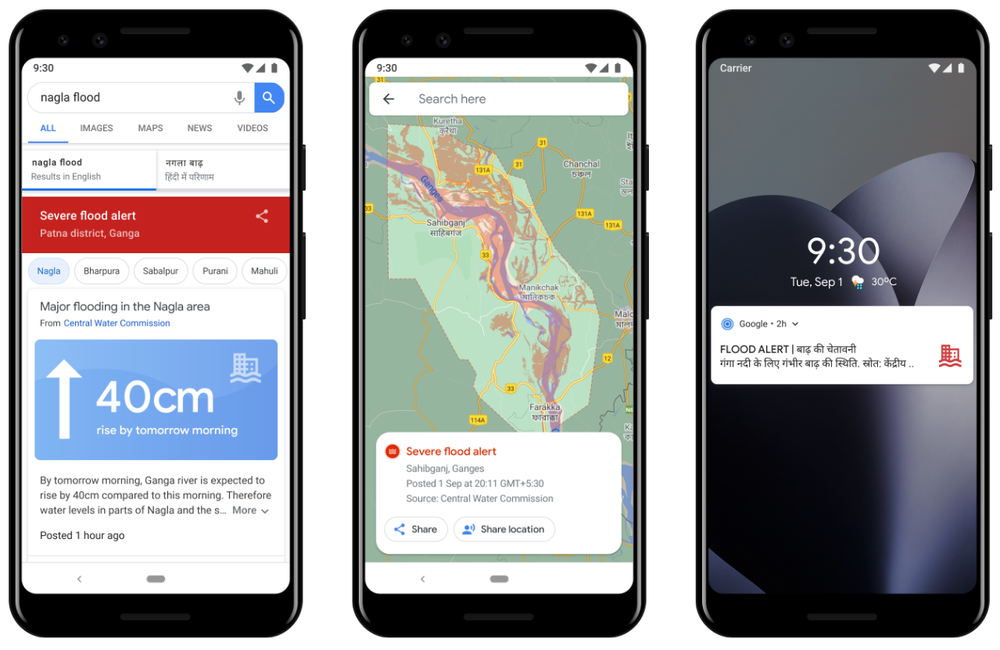
Flooding is the most common natural disaster on the planet, affecting the lives of hundreds of millions of people around the globe and causing around $10 billion in damages each year. Building on our work in previous years, earlier this week we announced some of our recent efforts to improve flood forecasting in India and Bangladesh, expanding coverage to more than 250 million people, and providing unprecedented lead time, accuracy and clarity.

To enable these breakthroughs, we have devised a new approach for inundation modeling, called a morphological inundation model, which combines physics-based modeling with machine learning (ML) to create more accurate and scalable inundation models in real-world settings. Additionally, our new alert-targeting model allows identifying areas at risk of flooding at unprecedented scale using end-to-end machine learning models and data that is publicly available globally. In this post, we also describe developments for the next generation of flood forecasting systems, called HydroNets (presented at ICLR AI for Earth Sciences and EGU this year), which is a new architecture specially built for hydrologic modeling across multiple basins, while still optimizing for accuracy at each location.

Forecasting Water Levels
The first step in a flood forecasting system is to identify whether a river is expected to flood. Hydrologic models (or gauge-to-gauge models) have long been used by governments and disaster management agencies to improve the accuracy and extend the lead time of their forecasts. These models receive inputs like precipitation or upstream gauge measurements of water level (i.e., the absolute elevation of the water above sea level) and output a forecast for the water level (or discharge) in the river at some time in the future.

The hydrologic model component of the flood forecasting system described in this week’s Keyword post doubled the lead time of flood alerts for areas covering more than 75 million people. These models not only increase lead time, but also provide unprecedented accuracy, achieving an R² score of more than 99% across all basins we cover, and predicting the water level within a 15 cm error bound more than 90% of the time. Once a river is predicted to reach flood level, the next step in generating actionable warnings is to convert the river level forecast into a prediction for how the floodplain will be affected.

Morphological Inundation Modeling
In prior work, we developed high quality elevation maps based on satellite imagery, and ran physics-based models to simulate water flow across these digital terrains, which allowed warnings with unprecedented resolution and accuracy in data-scarce regions. In collaboration with our satellite partners, Airbus, Maxar and Planet, we have now expanded the elevation maps to cover hundreds of millions of square kilometers. However, in order to scale up the coverage to such a large area while still retaining high accuracy, we had to re-invent how we develop inundation models.

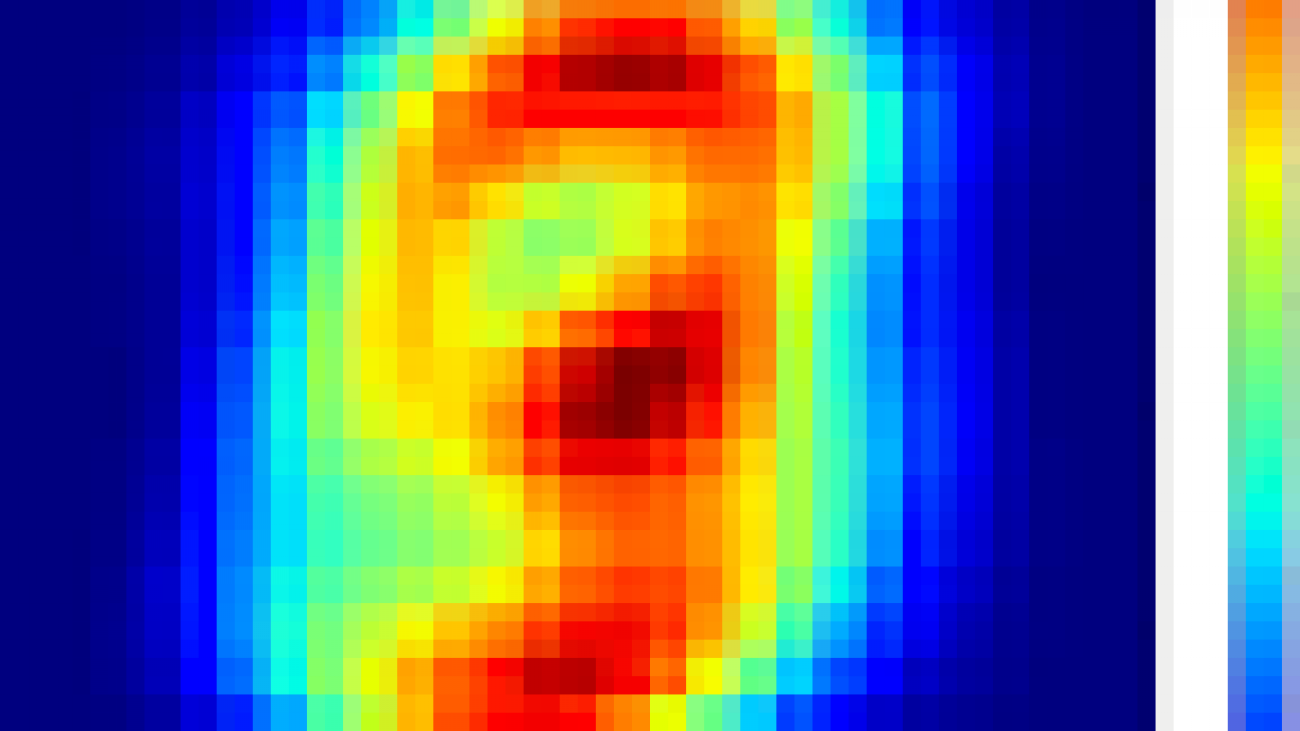
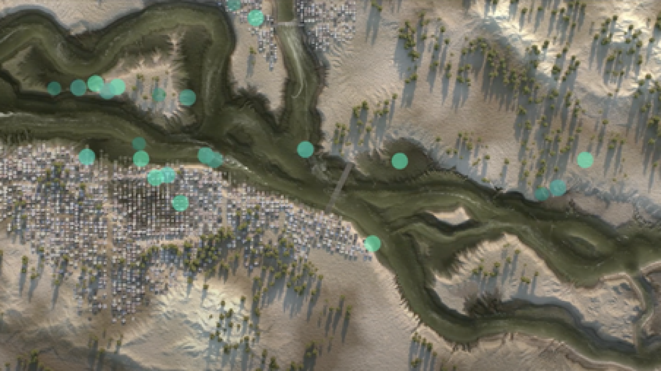
Inundation modeling estimates what areas will be flooded and how deep the water will be. This visualization conceptually shows how inundation could be simulated, how risk levels could be defined (represented by red and white colors), and how the model could be used to identify areas that should be warned (green dots).

Inundation modeling at scale suffers from three significant challenges. Due to the large areas involved and the resolution required for such models, they necessarily have high computational complexity. In addition, most global elevation maps don’t include riverbed bathymetry, which is important for accurate modeling. Finally, the errors in existing data, which may include gauge measurement errors, missing features in the elevation maps, and the like, need to be understood and corrected. Correcting such problems may require collecting additional high-quality data or fixing erroneous data manually, neither of which scale well.

Our new approach to inundation modeling, which we call a morphological model, addresses these issues by using several innovative tricks. Instead of modeling the complex behaviors of water flow in real time, we compute modifications to the morphology of the elevation map that allow one to simulate the inundation using simple physical principles, such as those describing hydrostatic systems.

First, we train a pure-ML model (devoid of physics-based information) to estimate the one-dimensional river profile from gauge measurements. The model takes as input the water level at a specific point on the river (the stream gauge) and outputs the river profile, which is the water level at all points in the river. We assume that if the gauge increases, the water level increases monotonically, i.e., the water level at other points in the river increases as well. We also assume that the absolute elevation of the river profile decreases downstream (i.e., the river flows downhill).

We then use this learned model and some heuristics to edit the elevation map to approximately “cancel out” the pressure gradient that would exist if that region were flooded. This new synthetic elevation map provides the foundation on which we model the flood behavior using a simple flood-fill algorithm. Finally, we match the resulting flooded map to the satellite-based flood extent with the original stream gauge measurement.

This approach abandons some of the realistic constraints of classical physics-based models, but in data scarce regions where existing methods currently struggle, its flexibility allows the model to automatically learn the correct bathymetry and fix various errors to which physics-based models are sensitive. This morphological model improves accuracy by 3%, which can significantly improve forecasts for large areas, while also allowing for much more rapid model development by reducing the need for manual modeling and correction.

Alert targeting
Many people reside in areas that are not covered by the morphological inundation models, yet access to accurate predictions are still urgently needed. To reach this population and to increase the impact of our flood forecasting models, we designed an end-to-end ML-based approach, using almost exclusively data that is globally publicly available, such as stream gauge measurements, public satellite imagery, and low resolution elevation maps. We train the model to use the data it is receiving to directly infer the inundation map in real time.

A direct ML approach from real-time measurements to inundation.

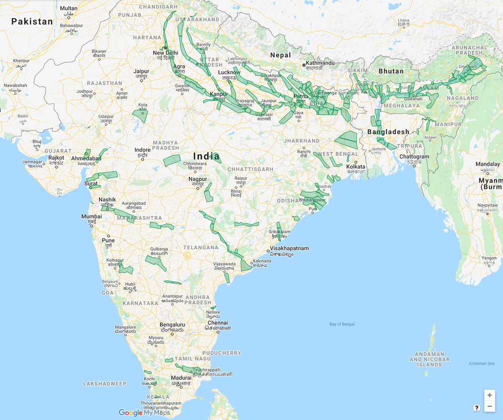
This approach works well “out of the box” when the model only needs to forecast an event that is within the range of events previously observed. Extrapolating to more extreme conditions is much more challenging. Nevertheless, proper use of existing elevation maps and real-time measurements can enable alerts that are more accurate than presently available for those in areas not covered by the more detailed morphological inundation models. Because this model is highly scalable, we were able to launch it across India after only a few months of work, and we hope to roll it out to many more countries soon.

Improving Water Levels Forecasting
In an effort to continue improving flood forecasting, we have developed HydroNets — a specialized deep neural network architecture built specifically for water levels forecasting — which allows us utilize some exciting recent advances in ML-based hydrology in a real-world operational setting. Two prominent features distinguish it from standard hydrologic models. First, it is able to differentiate between model components that generalize well between sites, such as the modeling of rainfall-runoff processes, and those that are specific to a given site, like the rating curve, which converts a predicted discharge volume into an expected water level. This enables the model to generalize well to different sites, while still fine-tuning its performance to each location. Second, HydroNets takes into account the structure of the river network being modeled, by training a large architecture that is actually a web of smaller neural networks, each representing a different location along the river. This allows neural networks that are modeling upstream sites to pass information encoded in embeddings to models of downstream sites, so that every model can know everything it needs without a drastic increase in parameters.

The animation below illustrates the structure and flow of information in HydroNets. The output from the modeling of upstream sub-basins is combined into a single representation of a given basin state. It is then processed by the shared model component, which is informed by all basins in the network, and passed on to the label prediction model, which calculates the water level (and the loss function). The output from this iteration of the network is then passed on to inform downstream models, and so on.

An illustration of the HydroNets architecture.

We’re incredibly excited about this progress, and are working hard on improving our systems further.

Acknowledgements
This work is a collaboration between many research teams at Google, and is part of our AI for Social Good efforts. We’d also like to thank our Geo and Policy teams, as well as Google.org.

Read More

Posted by Kurt Konolige, Software Engineer, Robotics at Google

Estimating the position and orientation of 3D objects is one of the core problems in computer vision applications that involve object-level perception, such as augmented reality and robotic manipulation. In these applications, it is important to know the 3D position of objects in the world, either to directly affect them, or to place simulated objects correctly around them. While there has been much research on this topic using machine learning (ML) techniques, especially Deep Nets, most have relied on the use of depth sensing devices, such as the Kinect, which give direct measurements of the distance to an object. For objects that are shiny or transparent, direct depth sensing does not work well. For example, the figure below includes a number of objects (left), two of which are transparent stars. A depth device does not find good depth values for the stars, and gives a very poor reconstruction of the actual 3D points (right).

Left: RGB image of transparent objects.  Right: A four-panel image showing the reconstructed depth for the scene on the left.The top row includes depth images and the bottom row presents the 3D point cloud. The left panels were reconstructed using a depth camera and the right panels are output from the ClearGrasp model.  Note that although ClearGrasp inpaints the depth of the stars, it mistakes the actual depth of the rightmost one.

One solution to this problem, such as that proposed by ClearGrasp, is to use a deep neural network to inpaint the corrupted depth map of the transparent objects. Given a single RGB-D image of transparent objects, ClearGrasp uses deep convolutional networks to infer surface normals, masks of transparent surfaces, and occlusion boundaries, which it uses to refine the initial depth estimates for all transparent surfaces in the scene (far right in the figure above). This approach is very promising, and allows scenes with transparent objects to be processed by pose-estimation methods that rely on depth.  But inpainting can be tricky, especially when trained completely with synthetic images, and can still result in errors in depth.

In “KeyPose: Multi-View 3D Labeling and Keypoint Estimation for Transparent Objects”, presented at CVPR 2020 in collaboration with the Stanford AI Lab, we describe an ML system that estimates the depth of transparent objects by directly predicting 3D keypoints. To train the system we gather a large real-world dataset of images of transparent objects in a semi-automated way, and efficiently label their pose using 3D keypoints selected by hand. We then train deep models (called KeyPose) to estimate the 3D keypoints end-to-end from monocular or stereo images, without explicitly computing depth. The models work on objects both seen and unseen during training, for both individual objects and categories of objects. While KeyPose can work with monocular images, the extra information available from stereo images allows it to improve its results by a factor of two over monocular image input, with typical errors from 5 mm to 10 mm, depending on the objects. It substantially improves over state-of-the-art in pose estimation for these objects, even when competing methods are provided with ground truth depth. We are releasing the dataset of keypoint-labeled transparent objects for use by the research community.

Real-World Transparent Object Dataset with 3D Keypoint Labels
To facilitate gathering large quantities of real-world images, we set up a robotic data-gathering system in which a robot arm moves through a trajectory while taking video with two devices, a stereo camera and the Kinect Azure depth camera.

Automated image sequence capture using a robot arm with a stereo camera and an Azure Kinect device.

The AprilTags on the target enable accurate tracing of the pose of the cameras. By hand-labelling only a few images in each video with 2D keypoints, we can extract 3D keypoints for all frames of the video using multi-view geometry, thus increasing the labelling efficiency by a factor of 100.

We captured imagery for 15 different transparent objects in five categories, using 10 different background textures and four different poses for each object, yielding a total of 600 video sequences comprising 48k stereo and depth images. We also captured the same images with an opaque version of the object, to provide accurate ground truth depth images. All the images are labelled with 3D keypoints. We are releasing this dataset of real-world images publicly, complementing the synthetic ClearGrasp dataset with which it shares similar objects.

KeyPose Algorithm Using Early Fusion Stereo
The idea of using stereo images directly for keypoint estimation was developed independently for this project; it has also appeared recently in the context of hand-tracking. The diagram below shows the basic idea: the two images from a stereo camera are cropped around the object and fed to the KeyPose network, which predicts a sparse set of 3D keypoints that represent the 3D pose of the object. The network is trained using supervision from the labelled 3D keypoints.

One of the key aspects of stereo KeyPose is the use of early fusion to intermix the stereo images, and allow the network to implicitly compute disparity, in contrast to late fusion, in which keypoints are predicted for each image separately, and then combined. As shown in the diagram below, the output of KeyPose is a 2D keypoint heatmap in the image plane along with a disparity (i.e., inverse depth) heatmap for each keypoint. The combination of these two heatmaps yields the 3D coordinate of the keypoint, for each keypoint.

Keypose system diagram. Stereo images are passed to a CNN model to produce a probability heatmap for each keypoint.  This heatmap yields 2D image coordinates U,V for the keypoint.  The CNN model also produces a disparity (inverse depth) heatmap for each keypoint, which when combined with the U,V coordinates, gives a 3D position (X,Y,Z).

When compared to late fusion or to monocular input, early fusion stereo typically is twice as accurate.

Results
The images below show qualitative results of KeyPose on individual objects. On the left is one of the original stereo images; in the middle are the predicted 3D keypoints projected onto the image. On the right, we visualize points from a 3D model of the bottle, placed at the pose determined by the predicted 3D keypoints. The network is efficient and accurate, predicting keypoints with an MAE of 5.2 mm for the bottle and 10.1 mm for the mug using just 5 ms on a standard GPU.

The following table shows results for KeyPose on category-level estimation. The test set used a background texture not seen by the training set. Note that the MAE varies from 5.8 mm to 9.9 mm, showing the accuracy of the method.

Quantitative comparison of KeyPose with the state-of-the-art DenseFusion system, on category-level data. We provide DenseFusion with two versions of depth, one from the transparent objects, and one from opaque objects. <2cm is the percent of estimates with errors less than 2 cm. MAE is the mean absolute error of the keypoints, in mm.

For a complete accounting of quantitative results, as well as, ablation studies, please see the paper and supplementary materials and the KeyPose website.

Conclusion
This work shows that it is possible to accurately estimate the 3D pose of transparent objects from RGB images without reliance on depth images. It validates the use of stereo images as input to an early fusion deep net, where the network is trained to extract sparse 3D keypoints directly from the stereo pair. We hope the availability of an extensive, labelled dataset of transparent objects will help to advance the field. Finally, while we used semi-automatic methods to efficiently label the dataset, we hope to employ self-supervision methods in future work to do away with manual labelling.

Acknowledgements
I want to thank my co-authors, Xingyu Liu of Stanford University, and Rico Jonschkowski and Anelia Angelova; as well the many who helped us through discussions during the project and paper writing, including Andy Zheng, Shuran Song, Vincent Vanhoucke, Pete Florence, and Jonathan Tompson.

Read More

Read More