 Bard can now help with programming and software development tasks, across more than 20 programming languages.Read More

Bard can now help with programming and software development tasks, across more than 20 programming languages.Read More
Time-series forecasting is an important research area that is critical to several scientific and industrial applications, like retail supply chain optimization, energy and traffic prediction, and weather forecasting. In retail use cases, for example, it has been observed that improving demand forecasting accuracy can meaningfully reduce inventory costs and increase revenue.
Modern time-series applications can involve forecasting hundreds of thousands of correlated time-series (e.g., demands of different products for a retailer) over long horizons (e.g., a quarter or year away at daily granularity). As such, time-series forecasting models need to satisfy the following key criterias:
A number of neural network–based solutions have been able to show good performance on benchmarks and also support the above criterion. However, these methods are typically slow to train and can be expensive for inference, especially for longer horizons.
In “Long-term Forecasting with TiDE: Time-series Dense Encoder”, we present an all multilayer perceptron (MLP) encoder-decoder architecture for time-series forecasting that achieves superior performance on long horizon time-series forecasting benchmarks when compared to transformer-based solutions, while being 5–10x faster. Then in “On the benefits of maximum likelihood estimation for Regression and Forecasting”, we demonstrate that using a carefully designed training loss function based on maximum likelihood estimation (MLE) can be effective in handling different data modalities. These two works are complementary and can be applied as a part of the same model. In fact, they will be available soon in Google Cloud AI’s Vertex AutoML Forecasting.
Deep learning has shown promise in time-series forecasting, outperforming traditional statistical methods, especially for large multivariate datasets. After the success of transformers in natural language processing (NLP), there have been several works evaluating variants of the Transformer architecture for long horizon (the amount of time into the future) forecasting, such as FEDformer and PatchTST. However, other work has suggested that even linear models can outperform these transformer variants on time-series benchmarks. Nonetheless, simple linear models are not expressive enough to handle auxiliary features (e.g., holiday features and promotions for retail demand forecasting) and non-linear dependencies on the past.
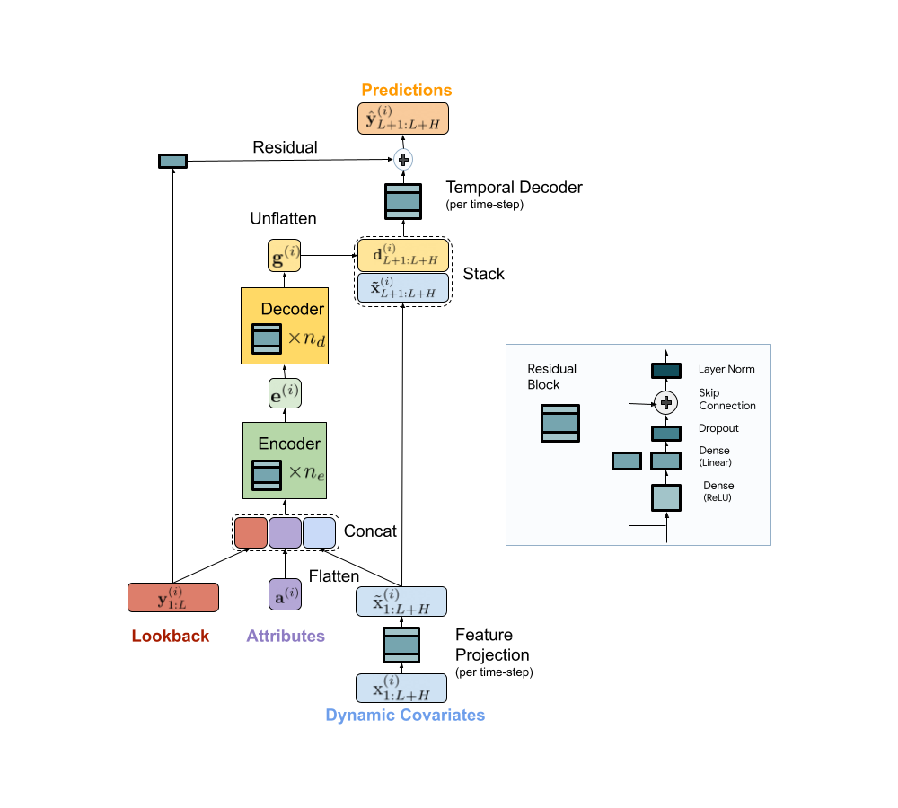
We present a scalable MLP-based encoder-decoder model for fast and accurate multi-step forecasting. Our model encodes the past of a time-series and all available features using an MLP encoder. Subsequently, the encoding is combined with future features using an MLP decoder to yield future predictions. The architecture is illustrated below.
 |
| TiDE model architecture for multi-step forecasting. |
TiDE is more than 10x faster in training compared to transformer-based baselines while being more accurate on benchmarks. Similar gains can be observed in inference as it only scales linearly with the length of the context (the number of time-steps the model looks back) and the prediction horizon. Below on the left, we show that our model can be 10.6% better than the best transformer-based baseline (PatchTST) on a popular traffic forecasting benchmark, in terms of test mean squared error (MSE). On the right, we show that at the same time our model can have much faster inference latency than PatchTST.
 |
| Left: MSE on the test set of a popular traffic forecasting benchmark. Right: inference time of TiDE and PatchTST as a function of the look-back length. |
Our research demonstrates that we can take advantage of MLP’s linear computational scaling with look-back and horizon sizes without sacrificing accuracy, while transformers scale quadratically in this situation.
In most forecasting applications the end user is interested in popular target metrics like the mean absolute percentage error (MAPE), weighted absolute percentage error (WAPE), etc. In such scenarios, the standard approach is to use the same target metric as the loss function while training. In “On the benefits of maximum likelihood estimation for Regression and Forecasting”, accepted at ICLR, we show that this approach might not always be the best. Instead, we advocate using the maximum likelihood loss for a carefully chosen family of distributions (discussed more below) that can capture inductive biases of the dataset during training. In other words, instead of directly outputting point predictions that minimize the target metric, the forecasting neural network predicts the parameters of a distribution in the chosen family that best explains the target data. At inference time, we can predict the statistic from the learned predictive distribution that minimizes the target metric of interest (e.g., the mean minimizes the MSE target metric while the median minimizes the WAPE). Further, we can also easily obtain uncertainty estimates of our forecasts, i.e., we can provide quantile forecasts by estimating the quantiles of the predictive distribution. In several use cases, accurate quantiles are vital, for instance, in demand forecasting a retailer might want to stock for the 90th percentile to guard against worst-case scenarios and avoid lost revenue.
The choice of the distribution family is crucial in such cases. For example, in the context of sparse count data, we might want to have a distribution family that can put more probability on zero, which is commonly known as zero-inflation. We propose a mixture of different distributions with learned mixture weights that can adapt to different data modalities. In the paper, we show that using a mixture of zero and multiple negative binomial distributions works well in a variety of settings as it can adapt to sparsity, multiple modalities, count data, and data with sub-exponential tails.
 |
| A mixture of zero and two negative binomial distributions. The weights of the three components, a1, a2 and a3, can be learned during training. |
We use this loss function for training Vertex AutoML models on the M5 forecasting competition dataset and show that this simple change can lead to a 6% gain and outperform other benchmarks in the competition metric, weighted root mean squared scaled error (WRMSSE).
| M5 Forecasting | WRMSSE |
| Vertex AutoML | 0.639 +/- 0.007 |
| Vertex AutoML with probabilistic loss | 0.581 +/- 0.007 |
| DeepAR | 0.789 +/- 0.025 |
| FEDFormer | 0.804 +/- 0.033 |
We have shown how TiDE, together with probabilistic loss functions, enables fast and accurate forecasting that automatically adapts to different data distributions and modalities and also provides uncertainty estimates for its predictions. It provides state-of-the-art accuracy among neural network–based solutions at a fraction of the cost of previous transformer-based forecasting architectures, for large-scale enterprise forecasting applications. We hope this work will also spur interest in revisiting (both theoretically and empirically) MLP-based deep time-series forecasting models.
This work is the result of a collaboration between several individuals across Google Research and Google Cloud, including (in alphabetical order): Pranjal Awasthi, Dawei Jia, Weihao Kong, Andrew Leach, Shaan Mathur, Petros Mol, Shuxin Nie, Ananda Theertha Suresh, and Rose Yu.
We announced some changes that will accelerate our progress in AI and help us develop more capable AI systems more safely and responsibly.Read More
Google sees AI as a foundational and transformational technology, with recent advances in generative AI technologies, such as LaMDA, PaLM, Imagen, Parti, MusicLM, and similar machine learning (ML) models, some of which are now being incorporated into our products. This transformative potential requires us to be responsible not only in how we advance our technology, but also in how we envision which technologies to build, and how we assess the social impact AI and ML-enabled technologies have on the world. This endeavor necessitates fundamental and applied research with an interdisciplinary lens that engages with — and accounts for — the social, cultural, economic, and other contextual dimensions that shape the development and deployment of AI systems. We must also understand the range of possible impacts that ongoing use of such technologies may have on vulnerable communities and broader social systems.
Our team, Technology, AI, Society, and Culture (TASC), is addressing this critical need. Research on the societal impacts of AI is complex and multi-faceted; no one disciplinary or methodological perspective can alone provide the diverse insights needed to grapple with the social and cultural implications of ML technologies. TASC thus leverages the strengths of an interdisciplinary team, with backgrounds ranging from computer science to social science, digital media and urban science. We use a multi-method approach with qualitative, quantitative, and mixed methods to critically examine and shape the social and technical processes that underpin and surround AI technologies. We focus on participatory, culturally-inclusive, and intersectional equity-oriented research that brings to the foreground impacted communities. Our work advances Responsible AI (RAI) in areas such as computer vision, natural language processing, health, and general purpose ML models and applications. Below, we share examples of our approach to Responsible AI and where we are headed in 2023.
 |
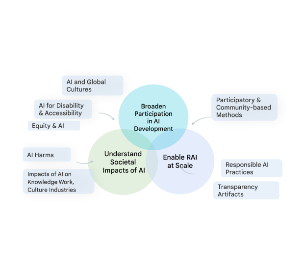
| A visual diagram of the various social, technical, and equity-oriented research areas that TASC studies to progress Responsible AI in a way that respects the complex relationships between AI and society. |
One of our key areas of research is the advancement of methods to make generative AI technologies more inclusive of and valuable to people globally, through community-engaged, and culturally-inclusive approaches. Toward this aim, we see communities as experts in their context, recognizing their deep knowledge of how technologies can and should impact their own lives. Our research champions the importance of embedding cross-cultural considerations throughout the ML development pipeline. Community engagement enables us to shift how we incorporate knowledge of what’s most important throughout this pipeline, from dataset curation to evaluation. This also enables us to understand and account for the ways in which technologies fail and how specific communities might experience harm. Based on this understanding we have created responsible AI evaluation strategies that are effective in recognizing and mitigating biases along multiple dimensions.
Our work in this area is vital to ensuring that Google’s technologies are safe for, work for, and are useful to a diverse set of stakeholders around the world. For example, our research on user attitudes towards AI, responsible interaction design, and fairness evaluations with a focus on the global south demonstrated the cross-cultural differences in the impact of AI and contributed resources that enable culturally-situated evaluations. We are also building cross-disciplinary research communities to examine the relationship between AI, culture, and society, through our recent and upcoming workshops on Cultures in AI/AI in Culture, Ethical Considerations in Creative Applications of Computer Vision, and Cross-Cultural Considerations in NLP.
Our recent research has also sought out perspectives of particular communities who are known to be less represented in ML development and applications. For example, we have investigated gender bias, both in natural language and in contexts such as gender-inclusive health, drawing on our research to develop more accurate evaluations of bias so that anyone developing these technologies can identify and mitigate harms for people with queer and non-binary identities.
We work to enable RAI at scale, by establishing industry-wide best practices for RAI across the development pipeline, and ensuring our technologies verifiably incorporate that best practice by default. This applied research includes responsible data production and analysis for ML development, and systematically advancing tools and practices that support practitioners in meeting key RAI goals like transparency, fairness, and accountability. Extending earlier work on Data Cards, Model Cards and the Model Card Toolkit, we released the Data Cards Playbook, providing developers with methods and tools to document appropriate uses and essential facts related to a dataset. Because ML models are often trained and evaluated on human-annotated data, we also advance human-centric research on data annotation. We have developed frameworks to document annotation processes and methods to account for rater disagreement and rater diversity. These methods enable ML practitioners to better ensure diversity in annotation of datasets used to train models, by identifying current barriers and re-envisioning data work practices.
We are now working to further broaden participation in ML model development, through approaches that embed a diversity of cultural contexts and voices into technology design, development, and impact assessment to ensure that AI achieves societal goals. We are also redefining responsible practices that can handle the scale at which ML technologies operate in today’s world. For example, we are developing frameworks and structures that can enable community engagement within industry AI research and development, including community-centered evaluation frameworks, benchmarks, and dataset curation and sharing.
In particular, we are furthering our prior work on understanding how NLP language models may perpetuate bias against people with disabilities, extending this research to address other marginalized communities and cultures and including image, video, and other multimodal models. Such models may contain tropes and stereotypes about particular groups or may erase the experiences of specific individuals or communities. Our efforts to identify sources of bias within ML models will lead to better detection of these representational harms and will support the creation of more fair and inclusive systems.
TASC is about studying all the touchpoints between AI and people — from individuals and communities, to cultures and society. For AI to be culturally-inclusive, equitable, accessible, and reflective of the needs of impacted communities, we must take on these challenges with inter- and multidisciplinary research that centers the needs of impacted communities. Our research studies will continue to explore the interactions between society and AI, furthering the discovery of new ways to develop and evaluate AI in order for us to develop more robust and culturally-situated AI technologies.
We would like to thank everyone on the team that contributed to this blog post. In alphabetical order by last name: Cynthia Bennett, Eric Corbett, Aida Mostafazadeh Davani, Emily Denton, Sunipa Dev, Fernando Diaz, Mark Díaz, Shaun Kane, Shivani Kapania, Michael Madaio, Vinodkumar Prabhakaran, Rida Qadri, Renee Shelby, Ding Wang, and Andrew Zaldivar. Also, we would like to thank Toju Duke and Marian Croak for their valuable feedback and suggestions.
Recently, differential privacy (DP) has emerged as a mathematically robust notion of user privacy for data aggregation and machine learning (ML), with practical deployments including the 2022 US Census and in industry. Over the last few years, we have open-sourced libraries for privacy-preserving analytics and ML and have been constantly enhancing their capabilities. Meanwhile, new algorithms have been developed by the research community for several analytic tasks involving private aggregation of data.
One such important data aggregation method is the heatmap. Heatmaps are popular for visualizing aggregated data in two or more dimensions. They are widely used in many fields including computer vision, image processing, spatial data analysis, bioinformatics, and more. Protecting the privacy of user data is critical for many applications of heatmaps. For example, heatmaps for gene microdata are based on private data from individuals. Similarly, a heatmap of popular locations in a geographic area are based on user location check-ins that need to be kept private.
Motivated by such applications, in “Differentially Private Heatmaps” (presented at AAAI 2023), we describe an efficient DP algorithm for computing heatmaps with provable guarantees and evaluate it empirically. At the core of our DP algorithm for heatmaps is a solution to the basic problem of how to privately aggregate sparse input vectors (i.e., input vectors with a small number of non-zero coordinates) with a small error as measured by the Earth Mover’s Distance (EMD). Using a hierarchical partitioning procedure, our algorithm views each input vector, as well as the output heatmap, as a probability distribution over a number of items equal to the dimension of the data. For the problem of sparse aggregation under EMD, we give an efficient algorithm with error asymptotically close to the best possible.
Our algorithm works by privatizing the aggregated distribution (obtained by averaging over all user inputs), which is sufficient for computing a final heatmap that is private due to the post-processing property of DP. This property ensures that any transformation of the output of a DP algorithm remains differentially private. Our main contribution is a new privatization algorithm for the aggregated distribution, which we will describe next.
The EMD measure, which is a distance-like measure of dissimilarity between two probability distributions originally proposed for computer vision tasks, is well-suited for heatmaps since it takes the underlying metric space into account and considers “neighboring” bins. EMD is used in a variety of applications including deep learning, spatial analysis, human mobility, image retrieval, face recognition, visual tracking, shape matching, and more.
To achieve DP, we need to add noise to the aggregated distribution. We would also like to preserve statistics at different scales of the grid to minimize the EMD error. So, we create a hierarchical partitioning of the grid, add noise at each level, and then recombine into the final DP aggregated distribution. In particular, the algorithm has the following steps:
 |
| In the first step, we take the (non-private) aggregated distribution (top left) and repeatedly divide it to create a quadtree. Then, we compute the total probability mass is each cell (bottom). |
 |
| In step 2, noise is added to each cell’s probability mass. Then in step 3, only top-w cells are kept (green) whereas the remaining cells are truncated (red). Finally, in the last step, we write a linear program on these top cells to reconstruct the aggregation distribution, which is now differentially private. |
We evaluate the performance of our algorithm in two different domains: real-world location check-in data and image saliency data. We consider as a baseline the ubiquitous Laplace mechanism, where we add Laplace noise to each cell, zero out any negative cells, and produce the heatmap from this noisy aggregate. We also consider a “thresholding” variant of this baseline that is more suited to sparse data: only keep top t% of the cell values (based on the probability mass in each cell) after noising while zeroing out the rest. To evaluate the quality of an output heatmap compared to the true heatmap, we use Pearson coefficient, KL-divergence, and EMD. Note that when the heatmaps are more similar, the first metric increases but the latter two decrease.
The locations dataset is obtained by combining two datasets, Gowalla and Brightkite, both of which contain check-ins by users of location-based social networks. We pre-processed this dataset to consider only check-ins in the continental US resulting in a final dataset consisting of ~500,000 check-ins by ~20,000 users. Considering the top cells (from an initial partitioning of the entire space into a 300 x 300 grid) that have check-ins from at least 200 unique users, we partition each such cell into subgrids with a resolution of ∆ × ∆ and assign each check-in to one of these subgrids.
In the first set of experiments, we fix ∆ = 256. We test the performance of our algorithm for different values of ε (the privacy parameter, where smaller ε means stronger DP guarantees), ranging from 0.1 to 10, by running our algorithms together with the baseline and its variants on all cells, randomly sampling a set of 200 users in each trial, and then computing the distance metrics between the true heatmap and the DP heatmap. The average of these metrics is presented below. Our algorithm (the red line) performs better than all versions of the baseline across all metrics, with improvements that are especially significant when ε is not too large or small (i.e., 0.2 ≤ ε ≤ 5).
 |
| Metrics averaged over 60 runs when varying ε for the location dataset. Shaded areas indicate 95% confidence interval. |
Next, we study the effect of varying the number n of users. By fixing a single cell (with > 500 users) and ε, we vary n from 50 to 500 users. As predicted by theory, our algorithms and the baseline perform better as n increases. However, the behavior of the thresholding variants of the baseline are less predictable.
We also run another experiment where we fix a single cell and ε, and vary the resolution ∆ from 64 to 256. In agreement with theory, our algorithm’s performance remains nearly constant for the entire range of ∆. However, the baseline suffers across all metrics as ∆ increases while the thresholding variants occasionally improve as ∆ increases.
 |
| Effect of the number of users and grid resolution on EMD. |
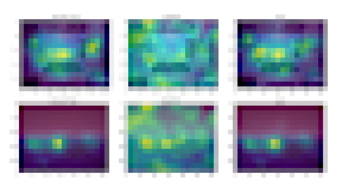
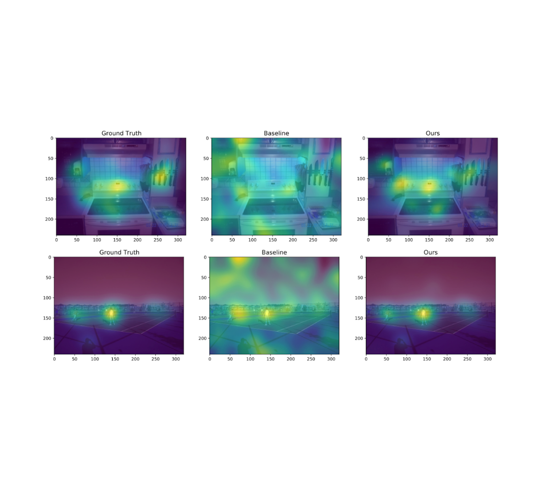
We also experiment on the Salicon image saliency dataset (SALICON). This dataset is a collection of saliency annotations on the Microsoft Common Objects in Context image database. We downsized the images to a fixed resolution of 320 × 240 and each [user, image] pair consists of a sequence of coordinates in the image where the user looked. We repeat the experiments described previously on 38 randomly sampled images (with ≥ 50 users each) from SALICON. As we can see from the examples below, the heatmap obtained by our algorithm is very close to the ground truth.
 |
| Example visualization of different algorithms for two different natural images from SALICON for ε = 10 and n = 50 users. The algorithms from left to right are: original heatmap (no privacy), baseline, and ours. |
Additional experimental results, including those on other datasets, metrics, privacy parameters and DP models, can be found in the paper.
We presented a privatization algorithm for sparse distribution aggregation under the EMD metric, which in turn yields an algorithm for producing privacy-preserving heatmaps. Our algorithm extends naturally to distributed models that can implement the Laplace mechanism, including the secure aggregation model and the shuffle model. This does not apply to the more stringent local DP model, and it remains an interesting open question to devise practical local DP heatmap/EMD aggregation algorithms for “moderate” number of users and privacy parameters.
This work was done jointly with Junfeng He, Kai Kohlhoff, Ravi Kumar, Pasin Manurangsi, and Vidhya Navalpakkam.
Derivatives play a central role in optimization and machine learning. By locally approximating a training loss, derivatives guide an optimizer toward lower values of the loss. Automatic differentiation frameworks such as TensorFlow, PyTorch, and JAX are an essential part of modern machine learning, making it feasible to use gradient-based optimizers to train very complex models.
But are derivatives all we need? By themselves, derivatives only tell us how a function behaves on an infinitesimal scale. To use derivatives effectively, we often need to know more than that. For example, to choose a learning rate for gradient descent, we need to know something about how the loss function behaves over a small but finite window. A finite-scale analogue of automatic differentiation, if it existed, could help us make such choices more effectively and thereby speed up training.
In our new paper “Automatically Bounding The Taylor Remainder Series: Tighter Bounds and New Applications“, we present an algorithm called AutoBound that computes polynomial upper and lower bounds on a given function, which are valid over a user-specified interval. We then begin to explore AutoBound’s applications. Notably, we present a meta-optimizer called SafeRate that uses the upper bounds computed by AutoBound to derive learning rates that are guaranteed to monotonically reduce a given loss function, without the need for time-consuming hyperparameter tuning. We are also making AutoBound available as an open-source library.
Given a function f and a reference point x0, AutoBound computes polynomial upper and lower bounds on f that hold over a user-specified interval called a trust region. Like Taylor polynomials, the bounding polynomials are equal to f at x0. The bounds become tighter as the trust region shrinks, and approach the corresponding Taylor polynomial as the trust region width approaches zero.
 |
| Automatically-derived quadratic upper and lower bounds on a one-dimensional function f, centered at x0=0.5. The upper and lower bounds are valid over a user-specified trust region, and become tighter as the trust region shrinks. |
Like automatic differentiation, AutoBound can be applied to any function that can be implemented using standard mathematical operations. In fact, AutoBound is a generalization of Taylor mode automatic differentiation, and is equivalent to it in the special case where the trust region has a width of zero.
To derive the AutoBound algorithm, there were two main challenges we had to address:
For a variety of commonly-used functions, we derive optimal polynomial upper and lower bounds in closed form. In this context, “optimal” means the bounds are as tight as possible, among all polynomials where only the maximum-degree coefficient differs from the Taylor series. Our theory applies to elementary functions, such as exp and log, and common neural network activation functions, such as ReLU and Swish. It builds upon and generalizes earlier work that applied only to quadratic bounds, and only for an unbounded trust region.
 |
| Optimal quadratic upper and lower bounds on the exponential function, centered at x0=0.5 and valid over the interval [0, 2]. |
To compute upper and lower bounds for arbitrary functions, we derived a generalization of the chain rule that operates on polynomial bounds. To illustrate the idea, suppose we have a function that can be written as
f(x) = g(h(x))
and suppose we already have polynomial upper and lower bounds on g and h. How do we compute bounds on f?
The key turns out to be representing the upper and lower bounds for a given function as a single polynomial whose highest-degree coefficient is an interval rather than a scalar. We can then plug the bound for h into the bound for g, and convert the result back to a polynomial of the same form using interval arithmetic. Under suitable assumptions about the trust region over which the bound on g holds, it can be shown that this procedure yields the desired bound on f.
 |
| The interval polynomial chain rule applied to the functions h(x) = sqrt(x) and g(y) = exp(y), with x0=0.25 and trust region [0, 0.5]. |
Our chain rule applies to one-dimensional functions, but also to multivariate functions, such as matrix multiplications and convolutions.
Using our new chain rule, AutoBound propagates interval polynomial bounds through a computation graph from the inputs to the outputs, analogous to forward-mode automatic differentiation.
 |
| Forward propagation of interval polynomial bounds for the function f(x) = exp(sqrt(x)). We first compute (trivial) bounds on x, then use the chain rule to compute bounds on sqrt(x) and exp(sqrt(x)). |
To compute bounds on a function f(x), AutoBound requires memory proportional to the dimension of x. For this reason, practical applications apply AutoBound to functions with a small number of inputs. However, as we will see, this does not prevent us from using AutoBound for neural network optimization.
What can we do with AutoBound that we couldn’t do with automatic differentiation alone?
Among other things, AutoBound can be used to automatically derive problem-specific, hyperparameter-free optimizers that converge from any starting point. These optimizers iteratively reduce a loss by first using AutoBound to compute an upper bound on the loss that is tight at the current point, and then minimizing the upper bound to obtain the next point.
 |
| Minimizing a one-dimensional logistic regression loss using quadratic upper bounds derived automatically by AutoBound. |
Optimizers that use upper bounds in this way are called majorization-minimization (MM) optimizers. Applied to one-dimensional logistic regression, AutoBound rederives an MM optimizer first published in 2009. Applied to more complex problems, AutoBound derives novel MM optimizers that would be difficult to derive by hand.
We can use a similar idea to take an existing optimizer such as Adam and convert it to a hyperparameter-free optimizer that is guaranteed to monotonically reduce the loss (in the full-batch setting). The resulting optimizer uses the same update direction as the original optimizer, but modifies the learning rate by minimizing a one-dimensional quadratic upper bound derived by AutoBound. We refer to the resulting meta-optimizer as SafeRate.
 |
| Performance of SafeRate when used to train a single-hidden-layer neural network on a subset of the MNIST dataset, in the full-batch setting. |
Using SafeRate, we can create more robust variants of existing optimizers, at the cost of a single additional forward pass that increases the wall time for each step by a small factor (about 2x in the example above).
In addition to the applications just discussed, AutoBound can be used for verified numerical integration and to automatically prove sharper versions of Jensen’s inequality, a fundamental mathematical inequality used frequently in statistics and other fields.
Bounding the Taylor remainder term automatically is not a new idea. A classical technique produces degree k polynomial bounds on a function f that are valid over a trust region [a, b] by first computing an expression for the kth derivative of f (using automatic differentiation), then evaluating this expression over [a,b] using interval arithmetic.
While elegant, this approach has some inherent limitations that can lead to very loose bounds, as illustrated by the dotted blue lines in the figure below.
 |
| Quadratic upper and lower bounds on the loss of a multi-layer perceptron with two hidden layers, as a function of the initial learning rate. The bounds derived by AutoBound are much tighter than those obtained using interval arithmetic evaluation of the second derivative. |
Taylor polynomials have been in use for over three hundred years, and are omnipresent in numerical optimization and scientific computing. Nevertheless, Taylor polynomials have significant limitations, which can limit the capabilities of algorithms built on top of them. Our work is part of a growing literature that recognizes these limitations and seeks to develop a new foundation upon which more robust algorithms can be built.
Our experiments so far have only scratched the surface of what is possible using AutoBound, and we believe it has many applications we have not discovered. To encourage the research community to explore such possibilities, we have made AutoBound available as an open-source library built on top of JAX. To get started, visit our GitHub repo.
This post is based on joint work with Josh Dillon. We thank Alex Alemi and Sergey Ioffe for valuable feedback on an earlier draft of the post.

Reinforcement learning (RL) can enable robots to learn complex behaviors through trial-and-error interaction, getting better and better over time. Several of our prior works explored how RL can enable intricate robotic skills, such as robotic grasping, multi-task learning, and even playing table tennis. Although robotic RL has come a long way, we still don’t see RL-enabled robots in everyday settings. The real world is complex, diverse, and changes over time, presenting a major challenge for robotic systems. However, we believe that RL should offer us an excellent tool for tackling precisely these challenges: by continually practicing, getting better, and learning on the job, robots should be able to adapt to the world as it changes around them.
In “Deep RL at Scale: Sorting Waste in Office Buildings with a Fleet of Mobile Manipulators”, we discuss how we studied this problem through a recent large-scale experiment, where we deployed a fleet of 23 RL-enabled robots over two years in Google office buildings to sort waste and recycling. Our robotic system combines scalable deep RL from real-world data with bootstrapping from training in simulation and auxiliary object perception inputs to boost generalization, while retaining the benefits of end-to-end training, which we validate with 4,800 evaluation trials across 240 waste station configurations.
When people don’t sort their trash properly, batches of recyclables can become contaminated and compost can be improperly discarded into landfills. In our experiment, a robot roamed around an office building searching for “waste stations” (bins for recyclables, compost, and trash). The robot was tasked with approaching each waste station to sort it, moving items between the bins so that all recyclables (cans, bottles) were placed in the recyclable bin, all the compostable items (cardboard containers, paper cups) were placed in the compost bin, and everything else was placed in the landfill trash bin. Here is what that looks like:
This task is not as easy as it looks. Just being able to pick up the vast variety of objects that people deposit into waste bins presents a major learning challenge. Robots also have to identify the appropriate bin for each object and sort them as quickly and efficiently as possible. In the real world, the robots can encounter a variety of situations with unique objects, like the examples from real office buildings below:
 |
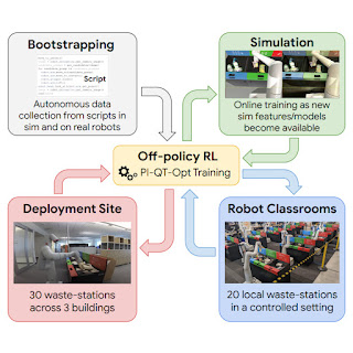
Learning on the job helps, but before even getting to that point, we need to bootstrap the robots with a basic set of skills. To this end, we use four sources of experience: (1) a set of simple hand-designed policies that have a very low success rate, but serve to provide some initial experience, (2) a simulated training framework that uses sim-to-real transfer to provide some initial bin sorting strategies, (3) “robot classrooms” where the robots continually practice at a set of representative waste stations, and (4) the real deployment setting, where robots practice in real office buildings with real trash.
 |
| A diagram of RL at scale. We bootstrap policies from data generated with a script (top-left). We then train a sim-to-real model and generate additional data in simulation (top-right). At each deployment cycle, we add data collected in our classrooms (bottom-right). We further deploy and collect data in office buildings (bottom-left). |
Our RL framework is based on QT-Opt, which we previously applied to learn bin grasping in laboratory settings, as well as a range of other skills. In simulation, we bootstrap from simple scripted policies and use RL, with a CycleGAN-based transfer method that uses RetinaGAN to make the simulated images appear more life-like.
From here, it’s off to the classroom. While real-world office buildings can provide the most representative experience, the throughput in terms of data collection is limited — some days there will be a lot of trash to sort, some days not so much. Our robots collect a large portion of their experience in “robot classrooms.” In the classroom shown below, 20 robots practice the waste sorting task:
While these robots are training in the classrooms, other robots are simultaneously learning on the job in 3 office buildings, with 30 waste stations:
In the end, we gathered 540k trials in the classrooms and 32.5k trials from deployment. Overall system performance improved as more data was collected. We evaluated our final system in the classrooms to allow for controlled comparisons, setting up scenarios based on what the robots saw during deployment. The final system could accurately sort about 84% of the objects on average, with performance increasing steadily as more data was added. In the real world, we logged statistics from three real-world deployments between 2021 and 2022, and found that our system could reduce contamination in the waste bins by between 40% and 50% by weight. Our paper provides further insights on the technical design, ablations studying various design decisions, and more detailed statistics on the experiments.
Our experiments showed that RL-based systems can enable robots to address real-world tasks in real office environments, with a combination of offline and online data enabling robots to adapt to the broad variability of real-world situations. At the same time, learning in more controlled “classroom” environments, both in simulation and in the real world, can provide a powerful bootstrapping mechanism to get the RL “flywheel” spinning to enable this adaptation. There is still a lot left to do: our final RL policies do not succeed every time, and larger and more powerful models will be needed to improve their performance and extend them to a broader range of tasks. Other sources of experience, including from other tasks, other robots, and even Internet videos may serve to further supplement the bootstrapping experience that we obtained from simulation and classrooms. These are exciting problems to tackle in the future. Please see the full paper here, and the supplementary video materials on the project webpage.
This research was conducted by multiple researchers at Robotics at Google and Everyday Robots, with contributions from Alexander Herzog, Kanishka Rao, Karol Hausman, Yao Lu, Paul Wohlhart, Mengyuan Yan, Jessica Lin, Montserrat Gonzalez Arenas, Ted Xiao, Daniel Kappler, Daniel Ho, Jarek Rettinghouse, Yevgen Chebotar, Kuang-Huei Lee, Keerthana Gopalakrishnan, Ryan Julian, Adrian Li, Chuyuan Kelly Fu, Bob Wei, Sangeetha Ramesh, Khem Holden, Kim Kleiven, David Rendleman, Sean Kirmani, Jeff Bingham, Jon Weisz, Ying Xu, Wenlong Lu, Matthew Bennice, Cody Fong, David Do, Jessica Lam, Yunfei Bai, Benjie Holson, Michael Quinlan, Noah Brown, Mrinal Kalakrishnan, Julian Ibarz, Peter Pastor, Sergey Levine and the entire Everyday Robots team.
Building models that solve a diverse set of tasks has become a dominant paradigm in the domains of vision and language. In natural language processing, large pre-trained models, such as PaLM, GPT-3 and Gopher, have demonstrated remarkable zero-shot learning of new language tasks. Similarly, in computer vision, models like CLIP and Flamingo have shown robust performance on zero-shot classification and object recognition. A natural next step is to use such tools to construct agents that can complete different decision-making tasks across many environments.
However, training such agents faces the inherent challenge of environmental diversity, since different environments operate with distinct state action spaces (e.g., the joint space and continuous controls in MuJoCo are fundamentally different from the image space and discrete actions in Atari). This environmental diversity hampers knowledge sharing, learning, and generalization across tasks and environments. Furthermore, it is difficult to construct reward functions across environments, as different tasks generally have different notions of success.
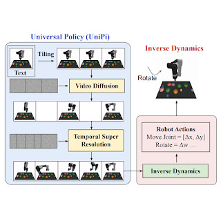
In “Learning Universal Policies via Text-Guided Video Generation”, we propose a Universal Policy (UniPi) that addresses environmental diversity and reward specification challenges. UniPi leverages text for expressing task descriptions and video (i.e., image sequences) as a universal interface for conveying action and observation behavior in different environments. Given an input image frame paired with text describing a current goal (i.e., the next high-level step), UniPi uses a novel video generator (trajectory planner) to generate video with snippets of what an agent’s trajectory should look like to achieve that goal. The generated video is fed into an inverse dynamics model that extracts underlying low-level control actions, which are then executed in simulation or by a real robot agent. We demonstrate that UniPi enables the use of language and video as a universal control interface for generalizing to novel goals and tasks across diverse environments.
 |
| Video policies generated by UniPi. |
 |
| UniPi may be applied to downstream multi-task settings that require combinatorial language generalization, long-horizon planning, or internet-scale knowledge. In the bottom example, UniPi takes the image of the white robot arm from the internet and generates video snippets according to the text description of the goal. |
To generate a valid and executable plan, a text-to-video model must synthesize a constrained video plan starting at the current observed image. We found it more effective to explicitly constrain a video synthesis model during training (as opposed to only constraining videos at sampling time) by providing the first frame of each video as explicit conditioning context.
At a high level, UniPi has four major components: 1) consistent video generation with first-frame tiling, 2) hierarchical planning through temporal super resolution, 3) flexible behavior synthesis, and 4) task-specific action adaptation. We explain the implementation and benefit of each component in detail below.
Existing text-to-video models like Imagen typically generate videos where the underlying environment state changes significantly throughout the duration. To construct an accurate trajectory planner, it is important that the environment remains consistent across all time points. We enforce environment consistency in conditional video synthesis by providing the observed image as additional context when denoising each frame in the synthesized video. To achieve context conditioning, UniPi directly concatenates each intermediate frame sampled from noise with the conditioned observed image across sampling steps, which serves as a strong signal to maintain the underlying environment state across time.
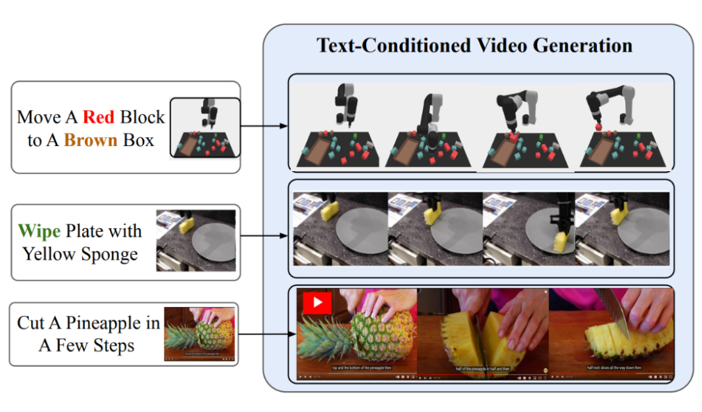 |
| Text-conditional video generation enables UniPi to train general purpose policies on a wide range of data sources (simulated, real robots and YouTube). |
When constructing plans in high-dimensional environments with long time horizons, directly generating a set of actions to reach a goal state quickly becomes intractable due to the exponential growth of the underlying search space as the plan gets longer. Planning methods often circumvent this issue by leveraging a natural hierarchy in planning. Specifically, planning methods first construct coarse plans (the intermediate key frames spread out across time) operating on low-dimensional states and actions, which are then refined into plans in the underlying state and action spaces.
Similar to planning, our conditional video generation procedure exhibits a natural temporal hierarchy. UniPi first generates videos at a coarse level by sparsely sampling videos (“abstractions”) of desired agent behavior along the time axis. UniPi then refines the videos to represent valid behavior in the environment by super-resolving videos across time. Meanwhile, coarse-to-fine super-resolution further improves consistency via interpolation between frames.
 |
| Given an input observation and text instruction, we plan a set of images representing agent behavior. Images are converted to actions using an inverse dynamics model. |
When planning a sequence of actions for a given sub-goal, one can readily incorporate external constraints to modulate a generated plan. Such test-time adaptability can be implemented by composing a probabilistic prior incorporating properties of the desired plan to specify desired constraints across the synthesized action trajectory, which is also compatible with UniPi. In particular, the prior can be specified using a learned classifier on images to optimize a particular task, or as a Dirac delta distribution on a particular image to guide a plan towards a particular set of states. To train the text-conditioned video generation model, we utilize the video diffusion algorithm, where pre-trained language features from the Text-To-Text Transfer Transformer (T5) are encoded.
Given a set of synthesized videos, we train a small task-specific inverse dynamics model to translate frames into a set of low-level control actions. This is independent from the planner and can be done on a separate, smaller and potentially suboptimal dataset generated by a simulator.
Given the input frame and text description of the current goal, the inverse dynamics model synthesizes image frames and generates a control action sequence that predicts the corresponding future actions. An agent then executes inferred low-level control actions via closed-loop control.
We measure the task success rate on novel language-based goals, and find that UniPi generalizes well to both seen and novel combinations of language prompts, compared to baselines such as Transformer BC, Trajectory Transformer (TT), and Diffuser.
 |
| UniPi generalizes well to both seen and novel combinations of language prompts in Place (e.g., “place X in Y”) and Relation (e.g., “place X to the left of Y”) tasks. |
Below, we illustrate generated videos on unseen combinations of goals. UniPi is able to synthesize a diverse set of behaviors that satisfy unseen language subgoals:
 |
| Generated videos for unseen language goals at test time. |
We measure the task success rate of UniPi and baselines on novel tasks not seen during training. UniPi again outperforms the baselines by a large margin:
 |
| UniPi generalizes well to new environments when trained on a set of different multi-task environments. |
Below, we illustrate generated videos on unseen tasks. UniPi is further able to synthesize a diverse set of behaviors that satisfy unseen language tasks:
 |
| Generated video plans on different new test tasks in the multitask setting. |
Below, we further illustrate generated videos given language instructions on unseen real images. Our approach is able to synthesize a diverse set of different behaviors which satisfy language instructions:
 |
Using internet pre-training enables UniPi to synthesize videos of tasks not seen during training. In contrast, a model trained from scratch incorrectly generates plans of different tasks:
 |
To evaluate the quality of videos generated by UniPi when pre-trained on non-robot data, we use the Fréchet Inception Distance (FID) and Fréchet Video Distance (FVD) metrics. We used Contrastive Language-Image Pre-training scores (CLIPScores) to measure the language-image alignment. We demonstrate that pre-trained UniPi achieves significantly higher FID and FVD scores and a better CLIPScore compared to UniPi without pre-training, suggesting that pre-training on non-robot data helps with generating plans for robots. We report the CLIPScore, FID, and VID scores for UniPi trained on Bridge data, with and without pre-training:
| Model (24×40) | CLIPScore ↑ | FID ↓ | FVD ↓ | ||||||||
| No pre-training | 24.43 ± 0.04 | 17.75 ± 0.56 | 288.02 ± 10.45 | ||||||||
| Pre-trained | 24.54 ± 0.03 | 14.54 ± 0.57 | 264.66 ± 13.64 |
| Using existing internet data improves video plan predictions under all metrics considered. |
The positive results of UniPi point to the broader direction of using generative models and the wealth of data on the internet as powerful tools to learn general-purpose decision making systems. UniPi is only one step towards what generative models can bring to decision making. Other examples include using generative foundation models to provide photorealistic or linguistic simulators of the world in which artificial agents can be trained indefinitely. Generative models as agents can also learn to interact with complex environments such as the internet, so that much broader and more complex tasks can eventually be automated. We look forward to future research in applying internet-scale foundation models to multi-environment and multi-embodiment settings.
We’d like to thank all remaining authors of the paper including Bo Dai, Hanjun Dai, Ofir Nachum, Joshua B. Tenenbaum, Dale Schuurmans, and Pieter Abbeel. We would like to thank George Tucker, Douglas Eck, and Vincent Vanhoucke for the feedback on this post and on the original paper.
Aging is a process that is characterized by physiological and molecular changes that increase an individual’s risk of developing diseases and eventually dying. Being able to measure and estimate the biological signatures of aging can help researchers identify preventive measures to reduce disease risk and impact. Researchers have developed “aging clocks” based on markers such as blood proteins or DNA methylation to measure individuals’ biological age, which is distinct from one’s chronological age. These aging clocks help predict the risk of age-related diseases. But because protein and methylation markers require a blood draw, non-invasive ways to find similar measures could make aging information more accessible.
Perhaps surprisingly, the features on our retinas reflect a lot about us. Images of the retina, which has vascular connections to the brain, are a valuable source of biological and physiological information. Its features have been linked to several aging-related diseases, including diabetic retinopathy, cardiovascular disease, and Alzheimer’s disease. Moreover, previous work from Google has shown that retinal images can be used to predict age, risk of cardiovascular disease, or even sex or smoking status. Could we extend those findings to aging, and maybe in the process identify a new, useful biomarker for human disease?
In a new paper “Longitudinal fundus imaging and its genome-wide association analysis provide evidence for a human retinal aging clock”, we show that deep learning models can accurately predict biological age from a retinal image and reveal insights that better predict age-related disease in individuals. We discuss how the model’s insights can improve our understanding of how genetic factors influence aging. Furthermore, we’re releasing the code modifications for these models, which build on ML frameworks for analyzing retina images that we have previously publicly released.
We trained a model to predict chronological age using hundreds of thousands of retinal images from a telemedicine-based blindness prevention program that were captured in primary care clinics and de-identified. A subset of these images has been used in a competition by Kaggle and academic publications, including prior Google work with diabetic retinopathy.
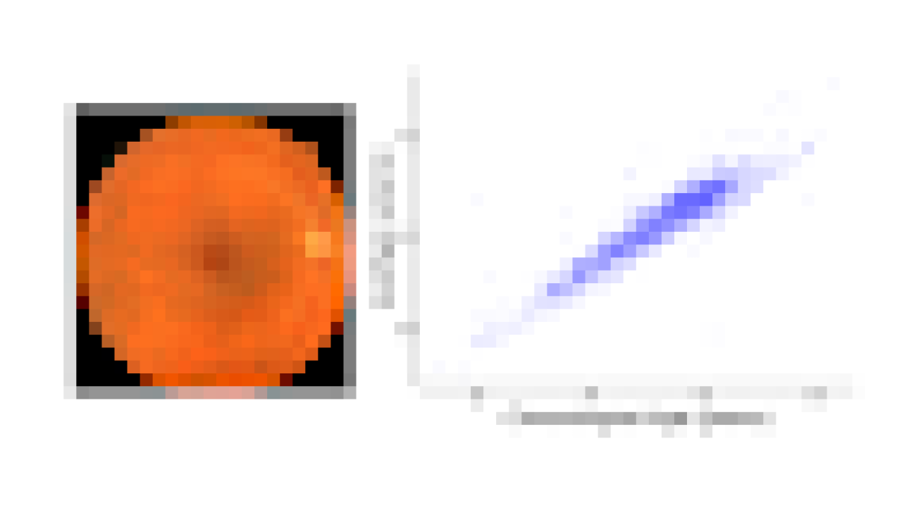
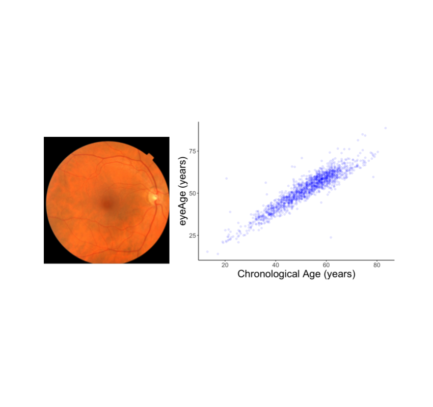
We evaluated the resulting model performance both on a held-out set of 50,000 retinal images and on a separate UKBiobank dataset containing approximately 120,000 images. The model predictions, named eyeAge, strongly correspond with the true chronological age of individuals (shown below; Pearson correlation coefficient of 0.87). This is the first time that retinal images have been used to create such an accurate aging clock.
 |
| Left: A retinal image showing the macula (dark spot in the middle), optic disc (bright spot at the right), and blood vessels (dark red lines extending from the optic disc). Right: Comparison of an individual’s true chronological age with the retina model predictions, “eyeAge”. |
Even though eyeAge correlates with chronological age well across many samples, the figure above also shows individuals for which the eyeAge differs substantially from chronological age, both in cases where the model predicts a value much younger or older than the chronological age. This could indicate that the model is learning factors in the retinal images that reflect real biological effects that are relevant to the diseases that become more prevalent with biological age.
To test whether this difference reflects underlying biological factors, we explored its correlation with conditions such as chronic obstructive pulmonary disease (COPD) and myocardial infarction and other biomarkers of health like systolic blood pressure. We observed that a predicted age higher than the chronological age, correlates with disease and biomarkers of health in these cases. For example, we showed a statistically significant (p=0.0028) correlation between eyeAge and all-cause mortality — that is a higher eyeAge was associated with a greater chance of death during the study.
To further explore the utility of the eyeAge model for generating biological insights, we related model predictions to genetic variants, which are available for individuals in the large UKBiobank study. Importantly, an individual’s germline genetics (the variants inherited from your parents) are fixed at birth, making this measure independent of age. This analysis generated a list of genes associated with accelerated biological aging (labeled in the figure below). The top identified gene from our genome-wide association study is ALKAL2, and interestingly the corresponding gene in fruit flies had previously been shown to be involved in extending life span in flies. Our collaborator, Professor Pankaj Kapahi from the Buck Institute for Research on Aging, found in laboratory experiments that reducing the expression of the gene in flies resulted in improved vision, providing an indication of ALKAL2 influence on the aging of the visual system.
 |
| Manhattan plot representing significant genes associated with gap between chronological age and eyeAge. Significant genes displayed as points above the dotted threshold line. |
Our eyeAge clock has many potential applications. As demonstrated above, it enables researchers to discover markers for aging and age-related diseases and to identify genes whose functions might be changed by drugs to promote healthier aging. It may also help researchers further understand the effects of lifestyle habits and interventions such as exercise, diet, and medication on an individual’s biological aging. Additionally, the eyeAge clock could be useful in the pharmaceutical industry for evaluating rejuvenation and anti-aging therapies. By tracking changes in the retina over time, researchers may be able to determine the effectiveness of these interventions in slowing or reversing the aging process.
Our approach to use retinal imaging for tracking biological age involves collecting images at multiple time points and analyzing them longitudinally to accurately predict the direction of aging. Importantly, this method is non-invasive and does not require specialized lab equipment. Our findings also indicate that the eyeAge clock, which is based on retinal images, is independent from blood-biomarker–based aging clocks. This allows researchers to study aging through another angle, and when combined with other markers, provides a more comprehensive understanding of an individual’s biological age. Also unlike current aging clocks, the less invasive nature of imaging (compared to blood tests) might enable eyeAge to be used for actionable biological and behavioral interventions.
We show that deep learning models can accurately predict an individual’s chronological age using only images of their retina. Moreover, when the predicted age differs from chronological age, this difference can identify accelerated onset of age-related disease. Finally, we show that the models learn insights which can improve our understanding of how genetic factors influence aging.
We’ve publicly released the code modifications used for these models which build on ML frameworks for analyzing retina images that we have previously publicly released.
It is our hope that this work will help scientists create better processes to identify disease and disease risk early, and lead to more effective drug and lifestyle interventions to promote healthy aging.
This work is the outcome of the combined efforts of multiple groups. We thank all contributors: Sara Ahadi, Boris Babenko, Cory McLean, Drew Bryant, Orion Pritchard, Avinash Varadarajan, Marc Berndl and Ali Bashir (Google Research), Kenneth Wilson, Enrique Carrera and Pankaj Kapahi (Buck Institute of Aging Research), and Ricardo Lamy and Jay Stewart (University of California, San Francisco). We would also like to thank Michelle Dimon and John Platt for reviewing the manuscript, and Preeti Singh for helping with publication logistics.
 A Google AI expert answers common questions about generative AI, large language models, machine learning and more.Read More