Posts in category: Google AI

Posted by Ashish Thapliyal, Software Engineer, and Jordi Pont-Tuset, Research Scientist, Google Research

Image captioning is the machine learning task of automatically generating a fluent natural language description for a given image. This task is important for improving accessibility for visually impaired users and is a core task in multimodal research encompassing both vision and language modeling.

However, datasets for image captioning are primarily available in English. Beyond that, there are only a few datasets covering a limited number of languages that represent just a small fraction of the world’s population. Further, these datasets feature images that severely under-represent the richness and diversity of cultures from across the globe. These aspects have hindered research on image captioning for a wide variety of languages, and directly hamper the deployment of accessibility solutions for a large potential audience around the world.

Today we present and make publicly available the Crossmodal 3600 (XM3600) image captioning evaluation dataset as a robust benchmark for multilingual image captioning that enables researchers to reliably compare research contributions in this emerging field. XM3600 provides 261,375 human-generated reference captions in 36 languages for a geographically diverse set of 3600 images. We show that the captions are of high quality and the style is consistent across languages.

Overview of the Crossmodal 3600 Dataset

Creating large training and evaluation datasets in multiple languages is a resource-intensive endeavor. Recent work has shown that it is feasible to build multilingual image captioning models trained on machine-translated data with English captions as the starting point. However, some of the most reliable automatic metrics for image captioning are much less effective when applied to evaluation sets with translated image captions, resulting in poorer agreement with human evaluations compared to the English case. As such, trustworthy model evaluation at present can only be based on extensive human evaluation. Unfortunately, such evaluations usually cannot be replicated across different research efforts, and therefore do not offer a fast and reliable mechanism to automatically evaluate multiple model parameters and configurations (e.g., model hill climbing) or to compare multiple lines of research.

XM3600 provides 261,375 human-generated reference captions in 36 languages for a geographically diverse set of 3600 images from the Open Images dataset. We measure the quality of generated captions by comparing them to the manually provided captions using the CIDEr metric, which ranges from 0 (unrelated to the reference captions) to 10 (perfectly matching the reference captions). When comparing pairs of models, we observed strong correlations between the differences in the CIDEr scores of the model outputs, and side-by-side human evaluations comparing the model outputs. , making XM3600 is a reliable tool for high-quality automatic comparisons between image captioning models on a wide variety of languages beyond English.

Language Selection

We chose 30 languages beyond English, roughly based on their percentage of web content. In addition, we chose an additional five languages that include under-resourced languages that have many native speakers or major native languages from continents that would not be covered otherwise. Finally, we also included English as a baseline, thus resulting in a total of 36 languages, as listed in the table below.

Image Selection

The images were selected from among those in the Open Images dataset that have location metadata. Since there are many regions where more than one language is spoken, and some areas are not well covered by these images, we designed an algorithm to maximize the correspondence between selected images and the regions where the targeted languages are spoken. The algorithm starts with the selection of images with geo-data corresponding to the languages for which we have the smallest pool (e.g., Persian) and processes them in increasing order of their candidate image pool size. If there aren’t enough images in an area where a language is spoken, then we gradually expand the geographic selection radius to: (i) a country where the language is spoken; (ii) a continent where the language is spoken; and, as last resort, (iii) from anywhere in the world. This strategy succeeded in providing our target number of 100 images from an appropriate region for most of the 36 languages, except for Persian (where 14 continent-level images are used) and Hindi (where all 100 images are at the global level, because the in-region images were assigned to Bengali and Telugu).

English Photo by Chris Sampson		Swahili Photo by Henrik Palm		Telugu Photo by rojypala
Cusco Quechua Photo by McKay Savage		Filipino Photo by Simon Schoeters		Chinese Photo by Stefan Krasowski

Caption Generation

In total, all 3600 images (100 images per language) are annotated in all 36 languages, each with an average of two annotations per language, yielding a total of 261,375 captions.

Annotators work in batches of 15 images. The first screen shows all 15 images with their captions in English as generated by a captioning model trained to output a consistent style of the form “<main salient objects> doing <activities> in the <environment>”, often with object attributes, such as a “smiling” person, “red” car, etc. The annotators are asked to rate the caption quality given guidelines for a 4-point scale from “excellent” to “bad”, plus an option for “not_enough_information”. This step forces the annotators to carefully assess caption quality and it primes them to internalize the style of the captions. The following screens show the images again but individually and without the English captions, and the annotators are asked to produce descriptive captions in the target language for each image.

The image batch size of 15 was chosen so that the annotators would internalize the style without remembering the exact captions. Thus, we expect the raters to generate captions based on the image content only and lacking translation artifacts. For example in the example shown below, the Spanish caption mentions “number 42” and the Thai caption mentions “convertibles”, none of which are mentioned in the English captions. The annotators were also provided with a protocol to use when creating the captions, thus achieving style consistency across languages.

Photo by Brian Solis		English		• A vintage sports car in a showroom with many other vintage sports cars
				• The branded classic cars in a row at display
		Spanish		• Automóvil clásico deportivo en exhibición de automóviles de galería — (Classic sports car in gallery car show)
				• Coche pequeño de carreras color plateado con el número 42 en una exhibición de coches — (Small silver racing car with the number 42 at a car show)
		Thai		• รถเปิดประทุนหลายสีจอดเรียงกันในที่จัดแสดง — (Multicolored convertibles line up in the exhibit)
				• รถแข่งวินเทจจอดเรียงกันหลายคันในงานจัดแสดง — (Several vintage racing cars line up at the show.)

Caption Quality and Statistics

We ran two to five pilot studies per language to troubleshoot the caption generation process and to ensure high quality captions. We then manually evaluated a random subset of captions. First we randomly selected a sample of 600 images. Then, to measure the quality of captions in a particular language, for each image, we selected for evaluation one of the manually generated captions. We found that:

• For 25 out of 36 languages, the percentage of captions rated as “Good” or “Excellent” is above 90%, and the rest are all above 70%.
• For 26 out of 36 languages, the percentage of captions rated as “Bad” is below 2%, and the rest are all below 5%.

For languages that use spaces to separate words, the number of words per caption can be as low as 5 or 6 for some agglutinative languages like Cusco Quechua and Czech, and as high as 18 for an analytic language like Vietnamese. The number of characters per caption also varies drastically — from mid-20s for Korean to mid-90s for Indonesian — depending on the alphabet and the script of the language.

Empirical Evaluation and Results

We empirically measured the ability of the XM3600 annotations to rank image captioning model variations by training four variations of a multilingual image captioning model and comparing the CIDEr differences of the models’ outputs over the XM3600 dataset for 30+ languages, to side-by-side human evaluations. We observed strong correlations between the CIDEr differences and the human evaluations. These results support the use of the XM3600 references as a means to achieve high-quality automatic comparisons between image captioning models on a wide variety of languages beyond English.

Recent Uses

Recently PaLI used XM3600 to evaluate model performance beyond English for image captioning, image-to-text retrieval and text-to-image retrieval. The key takeaways they found when evaluating on XM3600 were that multilingual captioning greatly benefits from scaling the PaLI models, especially for low-resource languages.

Acknowledgements

We would like to acknowledge the coauthors of this work: Xi Chen and Radu Soricut.

Read More

10:25

Read More

Read More

Posted by Zalán Borsos, Research Software Engineer, and Neil Zeghidour, Research Scientist, Google Research

Generating realistic audio requires modeling information represented at different scales. For example, just as music builds complex musical phrases from individual notes, speech combines temporally local structures, such as phonemes or syllables, into words and sentences. Creating well-structured and coherent audio sequences at all these scales is a challenge that has been addressed by coupling audio with transcriptions that can guide the generative process, be it text transcripts for speech synthesis or MIDI representations for piano. However, this approach breaks when trying to model untranscribed aspects of audio, such as speaker characteristics necessary to help people with speech impairments recover their voice, or stylistic components of a piano performance.

In “AudioLM: a Language Modeling Approach to Audio Generation”, we propose a new framework for audio generation that learns to generate realistic speech and piano music by listening to audio only. Audio generated by AudioLM demonstrates long-term consistency (e.g., syntax in speech, melody in music) and high fidelity, outperforming previous systems and pushing the frontiers of audio generation with applications in speech synthesis or computer-assisted music. Following our AI Principles, we’ve also developed a model to identify synthetic audio generated by AudioLM.

From Text to Audio Language Models

In recent years, language models trained on very large text corpora have demonstrated their exceptional generative abilities, from open-ended dialogue to machine translation or even common-sense reasoning. They have further shown their capacity to model other signals than texts, such as natural images. The key intuition behind AudioLM is to leverage such advances in language modeling to generate audio without being trained on annotated data.

However, some challenges need to be addressed when moving from text language models to audio language models. First, one must cope with the fact that the data rate for audio is significantly higher, thus leading to much longer sequences — while a written sentence can be represented by a few dozen characters, its audio waveform typically contains hundreds of thousands of values. Second, there is a one-to-many relationship between text and audio. This means that the same sentence can be rendered by different speakers with different speaking styles, emotional content and recording conditions.

To overcome both challenges, AudioLM leverages two kinds of audio tokens. First, semantic tokens are extracted from w2v-BERT, a self-supervised audio model. These tokens capture both local dependencies (e.g., phonetics in speech, local melody in piano music) and global long-term structure (e.g., language syntax and semantic content in speech, harmony and rhythm in piano music), while heavily downsampling the audio signal to allow for modeling long sequences.

However, audio reconstructed from these tokens demonstrates poor fidelity. To overcome this limitation, in addition to semantic tokens, we rely on acoustic tokens produced by a SoundStream neural codec, which capture the details of the audio waveform (such as speaker characteristics or recording conditions) and allow for high-quality synthesis. Training a system to generate both semantic and acoustic tokens leads simultaneously to high audio quality and long-term consistency.

Training an Audio-Only Language Model

AudioLM is a pure audio model that is trained without any text or symbolic representation of music. AudioLM models an audio sequence hierarchically, from semantic tokens up to fine acoustic tokens, by chaining several Transformer models, one for each stage. Each stage is trained for the next token prediction based on past tokens, as one would train a text language model. The first stage performs this task on semantic tokens to model the high-level structure of the audio sequence.

In the second stage, we concatenate the entire semantic token sequence, along with the past coarse acoustic tokens, and feed both as conditioning to the coarse acoustic model, which then predicts the future tokens. This step models acoustic properties such as speaker characteristics in speech or timbre in music.

In the third stage, we process the coarse acoustic tokens with the fine acoustic model, which adds even more detail to the final audio. Finally, we feed acoustic tokens to the SoundStream decoder to reconstruct a waveform.

After training, one can condition AudioLM on a few seconds of audio, which enables it to generate consistent continuation. In order to showcase the general applicability of the AudioLM framework, we consider two tasks from different audio domains:

• Speech continuation, where the model is expected to retain the speaker characteristics, prosody and recording conditions of the prompt while producing new content that is syntactically correct and semantically consistent.
• Piano continuation, where the model is expected to generate piano music that is coherent with the prompt in terms of melody, harmony and rhythm.

In the video below, you can listen to examples where the model is asked to continue either speech or music and generate new content that was not seen during training. As you listen, note that everything you hear after the gray vertical line was generated by AudioLM and that the model has never seen any text or musical transcription, but rather just learned from raw audio. We release more samples on this webpage.

To validate our results, we asked human raters to listen to short audio clips and decide whether it is an original recording of human speech or a synthetic continuation generated by AudioLM. Based on the ratings collected, we observed a 51.2% success rate, which is not statistically significantly different from the 50% success rate achieved when assigning labels at random. This means that speech generated by AudioLM is hard to distinguish from real speech for the average listener.

Our work on AudioLM is for research purposes and we have no plans to release it more broadly at this time. In alignment with our AI Principles, we sought to understand and mitigate the possibility that people could misinterpret the short speech samples synthesized by AudioLM as real speech. For this purpose, we trained a classifier that can detect synthetic speech generated by AudioLM with very high accuracy (98.6%). This shows that despite being (almost) indistinguishable to some listeners, continuations generated by AudioLM are very easy to detect with a simple audio classifier. This is a crucial first step to help protect against the potential misuse of AudioLM, with future efforts potentially exploring technologies such as audio “watermarking”.

Conclusion

We introduce AudioLM, a language modeling approach to audio generation that provides both long-term coherence and high audio quality. Experiments on speech generation show not only that AudioLM can generate syntactically and semantically coherent speech without any text, but also that continuations produced by the model are almost indistinguishable from real speech by humans. Moreover, AudioLM goes well beyond speech and can model arbitrary audio signals such as piano music. This encourages the future extensions to other types of audio (e.g., multilingual speech, polyphonic music, and audio events) as well as integrating AudioLM into an encoder-decoder framework for conditioned tasks such as text-to-speech or speech-to-speech translation.

Acknowledgments

The work described here was authored by Zalán Borsos, Raphaël Marinier, Damien Vincent, Eugene Kharitonov, Olivier Pietquin, Matt Sharifi, Olivier Teboul, David Grangier, Marco Tagliasacchi and Neil Zeghidour. We are grateful for all discussions and feedback on this work that we received from our colleagues at Google.

Read More

Posted by Fitsum Reda and Janne Kontkanen, Google Research

Frame interpolation is the process of synthesizing in-between images from a given set of images. The technique is often used for temporal up-sampling to increase the refresh rate of videos or to create slow motion effects. Nowadays, with digital cameras and smartphones, we often take several photos within a few seconds to capture the best picture. Interpolating between these “near-duplicate” photos can lead to engaging videos that reveal scene motion, often delivering an even more pleasing sense of the moment than the original photos.

Frame interpolation between consecutive video frames, which often have small motion, has been studied extensively. Unlike videos, however, the temporal spacing between near-duplicate photos can be several seconds, with commensurately large in-between motion, which is a major failing point of existing frame interpolation methods. Recent methods attempt to handle large motion by training on datasets with extreme motion, albeit with limited effectiveness on smaller motions.

In “FILM: Frame Interpolation for Large Motion”, published at ECCV 2022, we present a method to create high quality slow-motion videos from near-duplicate photos. FILM is a new neural network architecture that achieves state-of-the-art results in large motion, while also handling smaller motions well.

FILM interpolating between two near-duplicate photos to create a slow motion video.

FILM Model Overview

The FILM model takes two images as input and outputs a middle image. At inference time, we recursively invoke the model to output in-between images. FILM has three components: (1) A feature extractor that summarizes each input image with deep multi-scale (pyramid) features; (2) a bi-directional motion estimator that computes pixel-wise motion (i.e., flows) at each pyramid level; and (3) a fusion module that outputs the final interpolated image. We train FILM on regular video frame triplets, with the middle frame serving as the ground-truth for supervision.

A standard feature pyramid extraction on two input images. Features are processed at each level by a series of convolutions, which are then downsampled to half the spatial resolution and passed as input to the deeper level.

Scale-Agnostic Feature Extraction

Large motion is typically handled with hierarchical motion estimation using multi-resolution feature pyramids (shown above). However, this method struggles with small and fast-moving objects because they can disappear at the deepest pyramid levels. In addition, there are far fewer available pixels to derive supervision at the deepest level.

To overcome these limitations, we adopt a feature extractor that shares weights across scales to create a “scale-agnostic” feature pyramid. This feature extractor (1) allows the use of a shared motion estimator across pyramid levels (next section) by equating large motion at shallow levels with small motion at deeper levels, and (2) creates a compact network with fewer weights.

Specifically, given two input images, we first create an image pyramid by successively downsampling each image. Next, we use a shared U-Net convolutional encoder to extract a smaller feature pyramid from each image pyramid level (columns in the figure below). As the third and final step, we construct a scale-agnostic feature pyramid by horizontally concatenating features from different convolution layers that have the same spatial dimensions. Note that from the third level onwards, the feature stack is constructed with the same set of shared convolution weights (shown in the same color). This ensures that all features are similar, which allows us to continue to share weights in the subsequent motion estimator. The figure below depicts this process using four pyramid levels, but in practice, we use seven.

Bi-directional Flow Estimation

After feature extraction, FILM performs pyramid-based residual flow estimation to compute the flows from the yet-to-be-predicted middle image to the two inputs. The flow estimation is done once for each input, starting from the deepest level, using a stack of convolutions. We estimate the flow at a given level by adding a residual correction to the upsampled estimate from the next deeper level. This approach takes the following as its input: (1) the features from the first input at that level, and (2) the features of the second input after it is warped with the upsampled estimate. The same convolution weights are shared across all levels, except for the two finest levels.

Shared weights allow the interpretation of small motions at deeper levels to be the same as large motions at shallow levels, boosting the number of pixels available for large motion supervision. Additionally, shared weights not only enable the training of powerful models that may reach a higher peak signal-to-noise ratio (PSNR), but are also needed to enable models to fit into GPU memory for practical applications.

Fusion and Frame Generation

Once the bi-directional flows are estimated, we warp the two feature pyramids into alignment. We obtain a concatenated feature pyramid by stacking, at each pyramid level, the two aligned feature maps, the bi-directional flows and the input images. Finally, a U-Net decoder synthesizes the interpolated output image from the aligned and stacked feature pyramid.

FILM Architecture. FEATURE EXTRACTION: we extract scale-agnostic features. The features with matching colors are extracted using shared weights. FLOW ESTIMATION: we compute bi-directional flows using shared weights across the deeper pyramid levels and warp the features into alignment. FUSION: A U-Net decoder outputs the final interpolated frame.

Loss Functions

During training, we supervise FILM by combining three losses. First, we use the absolute L1 difference between the predicted and ground-truth frames to capture the motion between input images. However, this produces blurry images when used alone. Second, we use perceptual loss to improve image fidelity. This minimizes the L1 difference between the ImageNet pre-trained VGG-19 features extracted from the predicted and ground truth frames. Third, we use Style loss to minimize the L2 difference between the Gram matrix of the ImageNet pre-trained VGG-19 features. The Style loss enables the network to produce sharp images and realistic inpaintings of large pre-occluded regions. Finally, the losses are combined with weights empirically selected such that each loss contributes equally to the total loss.

Shown below, the combined loss greatly improves sharpness and image fidelity when compared to training FILM with L1 loss and VGG losses. The combined loss maintains the sharpness of the tree leaves.

FILM’s combined loss functions. L1 loss (left), L1 plus VGG loss (middle), and Style loss (right), showing significant sharpness improvements (green box).

Image and Video Results

We evaluate FILM on an internal near-duplicate photos dataset that exhibits large scene motion. Additionally, we compare FILM to recent frame interpolation methods: SoftSplat and ABME. FILM performs favorably when interpolating across large motion. Even in the presence of motion as large as 100 pixels, FILM generates sharp images consistent with the inputs.

Frame interpolation with SoftSplat (left), ABME (middle) and FILM (right) showing favorable image quality and temporal consistency.

Large motion interpolation. Top: 64x slow motion video. Bottom (left to right): The two input images blended, SoftSplat interpolation, ABME interpolation, and FILM interpolation. FILM captures the dog’s face while maintaining the background details.

Conclusion

We introduce FILM, a large motion frame interpolation neural network. At its core, FILM adopts a scale-agnostic feature pyramid that shares weights across scales, which allows us to build a “scale-agnostic” bi-directional motion estimator that learns from frames with normal motion and generalizes well to frames with large motion. To handle wide disocclusions caused by large scene motion, we supervise FILM by matching the Gram matrix of ImageNet pre-trained VGG-19 features, which results in realistic inpainting and crisp images. FILM performs favorably on large motion, while also handling small and medium motions well, and generates temporally smooth high quality videos.

Try It Out Yourself

You can try out FILM on your photos using the source code, which is now publicly available.

Acknowledgements

We would like to thank Eric Tabellion, Deqing Sun, Caroline Pantofaru, Brian Curless for their contributions. We thank Marc Comino Trinidad for his contributions on the scale-agnostic feature extractor, Orly Liba and Charles Herrmann for feedback on the text, Jamie Aspinall for the imagery in the paper, Dominik Kaeser, Yael Pritch, Michael Nechyba, William T. Freeman, David Salesin, Catherine Wah, and Ira Kemelmacher-Shlizerman for support. Thanks to Tom Small for creating the animated diagram in this post.

Read More

Posted by Srivatsan Krishnan, Student Researcher, and Aleksandra Faust, Senior Staff Research Scientist, Google Research, Brain Team

Deep reinforcement learning (RL) continues to make great strides in solving real-world sequential decision-making problems such as balloon navigation, nuclear physics, robotics, and games. Despite its promise, one of its limiting factors is long training times. While the current approach to speed up RL training on complex and difficult tasks leverages distributed training scaling up to hundreds or even thousands of computing nodes, it still requires the use of significant hardware resources which makes RL training expensive, while increasing its environmental impact. However, recent work [1, 2] indicates that performance optimizations on existing hardware can reduce the carbon footprint (i.e., total greenhouse gas emissions) of training and inference.

RL can also benefit from similar system optimization techniques that can reduce training time, improve hardware utilization and reduce carbon dioxide (CO₂) emissions. One such technique is quantization, a process that converts full-precision floating point (FP32) numbers to lower precision (int8) numbers and then performs computation using the lower precision numbers. Quantization can save memory storage cost and bandwidth for faster and more energy-efficient computation. Quantization has been successfully applied to supervised learning to enable edge deployments of machine learning (ML) models and achieve faster training. However, there remains an opportunity to apply quantization to RL training.

To that end, we present “QuaRL: Quantization for Fast and Environmentally SustainableReinforcement Learning”, published in the Transactions of Machine Learning Research journal, which introduces a new paradigm called ActorQ that applies quantization to speed up RL training by 1.5-5.4x while maintaining performance. Additionally, we demonstrate that compared to training in full-precision, the carbon footprint is also significantly reduced by a factor of 1.9-3.8x.

Applying Quantization to RL Training

In traditional RL training, a learner policy is applied to an actor, which uses the policy to explore the environment and collect data samples. The samples collected by the actor are then used by the learner to continuously refine the initial policy. Periodically, the policy trained on the learner side is used to update the actor’s policy. To apply quantization to RL training, we develop the ActorQ paradigm. ActorQ performs the same sequence described above, with one key difference being that the policy update from learner to actors is quantized, and the actor explores the environment using the int8 quantized policy to collect samples.

Applying quantization to RL training in this fashion has two key benefits. First, it reduces the memory footprint of the policy. For the same peak bandwidth, less data is transferred between learners and actors, which reduces the communication cost for policy updates from learners to actors. Second, the actors perform inference on the quantized policy to generate actions for a given environment state. The quantized inference process is much faster when compared to performing inference in full precision.

An overview of traditional RL training (left) and ActorQ RL training (right).

In ActorQ, we use the ACME distributed RL framework. The quantizer block performs uniform quantization that converts the FP32 policy to int8. The actor performs inference using optimized int8 computations. Though we use uniform quantization when designing the quantizer block, we believe that other quantization techniques can replace uniform quantization and produce similar results. The samples collected by the actors are used by the learner to train a neural network policy. Periodically the learned policy is quantized by the quantizer block and broadcasted to the actors.

Quantization Improves RL Training Time and Performance

We evaluate ActorQ in a range of environments, including the Deepmind Control Suite and the OpenAI Gym. We demonstrate the speed-up and improved performance of D4PG and DQN. We chose D4PG as it was the best learning algorithm in ACME for Deepmind Control Suite tasks, and DQN is a widely used and standard RL algorithm.

We observe a significant speedup (between 1.5x and 5.41x) in training RL policies. More importantly, performance is maintained even when actors perform int8 quantized inference. The figures below demonstrate this for the D4PG and DQN agents for Deepmind Control Suite and OpenAI Gym tasks.

A comparison of RL training using the FP32 policy (q=32) and the quantized int8 policy (q=8) for D4PG agents on various Deepmind Control Suite tasks. Quantization achieves speed-ups of 1.5x to 3.06x.

A comparison of RL training using the FP32 policy (q=32) and the quantized int8 policy (q=8) for DQN agents in the OpenAI Gym environment. Quantization achieves a speed-up of 2.2x to 5.41x.

Quantization Reduces Carbon Emission

Applying quantization in RL using ActorQ improves training time without affecting performance. The direct consequence of using the hardware more efficiently is a smaller carbon footprint. We measure the carbon footprint improvement by taking the ratio of carbon emission when using the FP32 policy during training over the carbon emission when using the int8 policy during training.

In order to measure the carbon emission for the RL training experiment, we use the experiment-impact-tracker proposed in prior work. We instrument the ActorQ system with carbon monitor APIs to measure the energy and carbon emissions for each training experiment.

Compared to the carbon emission when running in full precision (FP32), we observe that the quantization of policies reduces the carbon emissions anywhere from 1.9x to 3.76x, depending on the task. As RL systems are scaled to run on thousands of distributed hardware cores and accelerators, we believe that the absolute carbon reduction (measured in kilograms of CO₂) can be quite significant.

Carbon emission comparison between training using a FP32 policy and an int8 policy. The X-axis scale is normalized to the carbon emissions of the FP32 policy. Shown by the red bars greater than 1, ActorQ reduces carbon emissions.

Conclusion and Future Directions

We introduce ActorQ, a novel paradigm that applies quantization to RL training and achieves speed-up improvements of 1.5-5.4x while maintaining performance. Additionally, we demonstrate that ActorQ can reduce RL training’s carbon footprint by a factor of 1.9-3.8x compared to training in full-precision without quantization.

ActorQ demonstrates that quantization can be effectively applied to many aspects of RL, from obtaining high-quality and efficient quantized policies to reducing training times and carbon emissions. As RL continues to make great strides in solving real-world problems, we believe that making RL training sustainable will be critical for adoption. As we scale RL training to thousands of cores and GPUs, even a 50% improvement (as we have experimentally demonstrated) will generate significant savings in absolute dollar cost, energy, and carbon emissions. Our work is the first step toward applying quantization to RL training to achieve efficient and environmentally sustainable training.

While our design of the quantizer in ActorQ relied on simple uniform quantization, we believe that other forms of quantization, compression and sparsity can be applied (e.g., distillation, sparsification, etc.). We hope that future work will consider applying more aggressive quantization and compression methods, which may yield additional benefits to the performance and accuracy tradeoff obtained by the trained RL policies.

Acknowledgments

We would like to thank our co-authors Max Lam, Sharad Chitlangia, Zishen Wan, and Vijay Janapa Reddi (Harvard University), and Gabriel Barth-Maron (DeepMind), for their contribution to this work. We also thank the Google Cloud team for providing research credits to seed this work.

Read More

Posted by Jeremy Maitin-Shepard and Laramie Leavitt, Software Engineers, Connectomics at Google

Many exciting contemporary applications of computer science and machine learning (ML) manipulate multidimensional datasets that span a single large coordinate system, for example, weather modeling from atmospheric measurements over a spatial grid or medical imaging predictions from multi-channel image intensity values in a 2d or 3d scan. In these settings, even a single dataset may require terabytes or petabytes of data storage. Such datasets are also challenging to work with as users may read and write data at irregular intervals and varying scales, and are often interested in performing analyses using numerous machines working in parallel.

Today we are introducing TensorStore, an open-source C++ and Python software library designed for storage and manipulation of n-dimensional data that:

• Provides a uniform API for reading and writing multiple array formats, including zarr and N5.
• Natively supports multiple storage systems, including Google Cloud Storage, local and network filesystems, HTTP servers, and in-memory storage.
• Supports read/writeback caching and transactions, with strong atomicity, isolation, consistency, and durability (ACID) guarantees.
• Supports safe, efficient access from multiple processes and machines via optimistic concurrency.
• Offers an asynchronous API to enable high-throughput access even to high-latency remote storage.
• Provides advanced, fully composable indexing operations and virtual views.

TensorStore has already been used to solve key engineering challenges in scientific computing (e.g., management and processing of large datasets in neuroscience, such as peta-scale 3d electron microscopy data and “4d” videos of neuronal activity). TensorStore has also been used in the creation of large-scale machine learning models such as PaLM by addressing the problem of managing model parameters (checkpoints) during distributed training.

Familiar API for Data Access and Manipulation

TensorStore provides a simple Python API for loading and manipulating large array data. In the following example, we create a TensorStore object that represents a 56 trillion voxel 3d image of a fly brain and access a small 100×100 patch of the data as a NumPy array:

>>> import tensorstore as ts
>>> import numpy as np

# Create a TensorStore object to work with fly brain data.
>>> dataset = ts.open({
...     'driver':
...         'neuroglancer_precomputed',
...     'kvstore':
...         'gs://neuroglancer-janelia-flyem-hemibrain/' + 
...         'v1.1/segmentation/',
... }).result()

# Create a 3-d view (remove singleton 'channel' dimension):
>>> dataset_3d = dataset[ts.d['channel'][0]]
>>> dataset_3d.domain
{ "x": [0, 34432), "y": [0, 39552), "z": [0, 41408) }

# Convert a 100x100x1 slice of the data to a numpy ndarray
>>> slice = np.array(dataset_3d[15000:15100, 15000:15100, 20000])

Crucially, no actual data is accessed or stored in memory until the specific 100×100 slice is requested; hence arbitrarily large underlying datasets can be loaded and manipulated without having to store the entire dataset in memory, using indexing and manipulation syntax largely identical to standard NumPy operations. TensorStore also provides extensive support for advanced indexing features, including transforms, alignment, broadcasting, and virtual views (data type conversion, downsampling, lazily on-the-fly generated arrays).

The following example demonstrates how TensorStore can be used to create a zarr array, and how its asynchronous API enables higher throughput:

>>> import tensorstore as ts
>>> import numpy as np

>>> # Create a zarr array on the local filesystem
>>> dataset = ts.open({
...     'driver': 'zarr',
...     'kvstore': 'file:///tmp/my_dataset/',
... },
... dtype=ts.uint32,
... chunk_layout=ts.ChunkLayout(chunk_shape=[256, 256, 1]),
... create=True,
... shape=[5000, 6000, 7000]).result()

>>> # Create two numpy arrays with example data to write.
>>> a = np.arange(100*200*300, dtype=np.uint32).reshape((100, 200, 300))
>>> b = np.arange(200*300*400, dtype=np.uint32).reshape((200, 300, 400))

>>> # Initiate two asynchronous writes, to be performed concurrently.
>>> future_a = dataset[1000:1100, 2000:2200, 3000:3300].write(a)
>>> future_b = dataset[3000:3200, 4000:4300, 5000:5400].write(b)

>>> # Wait for the asynchronous writes to complete
>>> future_a.result()
>>> future_b.result()

Safe and Performant Scaling

Processing and analyzing large numerical datasets requires significant computational resources. This is typically achieved through parallelization across numerous CPU or accelerator cores spread across many machines. Therefore a fundamental goal of TensorStore has been to enable parallel processing of individual datasets that is both safe (i.e., avoids corruption or inconsistencies arising from parallel access patterns) and high performance (i.e., reading and writing to TensorStore is not a bottleneck during computation). In fact, in a test within Google’s datacenters, we found nearly linear scaling of read and write performance as the number of CPUs was increased:

Read and write performance for a TensorStore dataset in zarr format residing on Google Cloud Storage (GCS) accessed concurrently using a variable number of single-core compute tasks in Google data centers. Both read and write performance scales nearly linearly with the number of compute tasks.

Performance is achieved by implementing core operations in C++, extensive use of multithreading for operations such as encoding/decoding and network I/O, and partitioning large datasets into much smaller units through chunking to enable efficiently reading and writing subsets of the entire dataset. TensorStore also provides configurable in-memory caching (which reduces slower storage system interactions for frequently accessed data) and an asynchronous API that enables a read or write operation to continue in the background while a program completes other work.

Safety of parallel operations when many machines are accessing the same dataset is achieved through the use of optimistic concurrency, which maintains compatibility with diverse underlying storage layers (including Cloud storage platforms, such as GCS, as well as local filesystems) without significantly impacting performance. TensorStore also provides strong ACID guarantees for all individual operations executing within a single runtime.

To make distributed computing with TensorStore compatible with many existing data processing workflows, we have also integrated TensorStore with parallel computing libraries such as Apache Beam (example code) and Dask (example code).

Use Case: Language Models

An exciting recent development in ML is the emergence of more advanced language models such as PaLM. These neural networks contain hundreds of billions of parameters and exhibit some surprising capabilities in natural language understanding and generation. These models also push the limits of computational infrastructure; in particular, training a language model such as PaLM requires thousands of TPUs working in parallel.

One challenge that arises during this training process is efficiently reading and writing the model parameters. Training is distributed across many separate machines, but parameters must be regularly saved to a single object (“checkpoint”) on a permanent storage system without slowing down the overall training process. Individual training jobs must also be able to read just the specific set of parameters they are concerned with in order to avoid the overhead that would be required to load the entire set of model parameters (which could be hundreds of gigabytes).

TensorStore has already been used to address these challenges. It has been applied to manage checkpoints associated with large-scale (“multipod”) models trained with JAX (code example) and has been integrated with frameworks such as T5X (code example) and Pathways. Model parallelism is used to partition the full set of parameters, which can occupy more than a terabyte of memory, over hundreds of TPUs. Checkpoints are stored in zarr format using TensorStore, with a chunk structure chosen to allow the partition for each TPU to be read and written independently in parallel.

When saving a checkpoint, each model parameter is written using TensorStore in zarr format using a chunk grid that further subdivides the grid used to partition the parameter over TPUs. The host machines write in parallel the zarr chunks for each of the partitions assigned to TPUs attached to that host. Using TensorStore’s asynchronous API, training proceeds even while the data is still being written to persistent storage. When resuming from a checkpoint, each host reads only the chunks that make up the partitions assigned to that host.

Use Case: 3D Brain Mapping

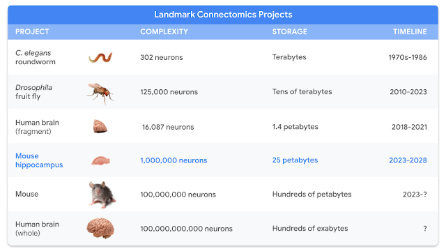
The field of synapse-resolution connectomics aims to map the wiring of animal and human brains at the detailed level of individual synaptic connections. This requires imaging the brain at extremely high resolution (nanometers) over fields of view of up to millimeters or more, which yields datasets that can span petabytes in size. In the future these datasets may extend to exabytes as scientists contemplate mapping entire mouse or primate brains. However, even current datasets pose significant challenges related to storage, manipulation, and processing; in particular, even a single brain sample may require millions of gigabytes with a coordinate system (pixel space) of hundreds of thousands pixels in each dimension.

We have used TensorStore to solve computational challenges associated with large-scale connectomic datasets. Specifically, TensorStore has managed some of the largest and most widely accessed connectomic datasets, with Google Cloud Storage as the underlying object storage system. For example, it has been applied to the human cortex “h01” dataset, which is a 3d nanometer-resolution image of human brain tissue. The raw imaging data is 1.4 petabytes (roughly 500,000 * 350,000 * 5,000 pixels large, and is further associated with additional content such as 3d segmentations and annotations that reside in the same coordinate system. The raw data is subdivided into individual chunks 128x128x16 pixels large and stored in the “Neuroglancer precomputed” format, which is optimized for web-based interactive viewing and can be easily manipulated from TensorStore.

A fly brain reconstruction for which the underlying data can be easily accessed and manipulated using TensorStore.

Getting Started

To get started using the TensorStore Python API, you can install the tensorstore PyPI package using:

pip install tensorstore

Refer to the tutorials and API documentation for usage details. For other installation options and for using the C++ API, refer to installation instructions.

Acknowledgements

Thanks to Tim Blakely, Viren Jain, Yash Katariya, Jan-Matthis Luckmann, Michał Januszewski, Peter Li, Adam Roberts, Brain Williams, and Hector Yee from Google Research, and Davis Bennet, Stuart Berg, Eric Perlman, Stephen Plaza, and Juan Nunez-Iglesias from the broader scientific community for valuable feedback on the design, early testing and debugging.

Read More

Posted by Carlos Esteves and Ameesh Makadia, Research Scientists, Google Research

A long-standing problem in the intersection of computer vision and computer graphics, view synthesis is the task of creating new views of a scene from multiple pictures of that scene. This has received increased attention [1, 2, 3] since the introduction of neural radiance fields (NeRF). The problem is challenging because to accurately synthesize new views of a scene, a model needs to capture many types of information — its detailed 3D structure, materials, and illumination — from a small set of reference images.

In this post, we present recently published deep learning models for view synthesis. In “Light Field Neural Rendering” (LFNR), presented at CVPR 2022, we address the challenge of accurately reproducing view-dependent effects by using transformers that learn to combine reference pixel colors. Then in “Generalizable Patch-Based Neural Rendering” (GPNR), to be presented at ECCV 2022, we address the challenge of generalizing to unseen scenes by using a sequence of transformers with canonicalized positional encoding that can be trained on a set of scenes to synthesize views of new scenes. These models have some unique features. They perform image-based rendering, combining colors and features from the reference images to render novel views. They are purely transformer-based, operating on sets of image patches, and they leverage a 4D light field representation for positional encoding, which helps to model view-dependent effects.

We train deep learning models that are able to produce new views of a scene given a few images of it. These models are particularly effective when handling view-dependent effects like the refractions and translucency on the test tubes. This animation is compressed; see the original-quality renderings here. Source: Lab scene from the NeX/Shiny dataset.

Overview

The input to the models consists of a set of reference images and their camera parameters (focal length, position, and orientation in space), along with the coordinates of the target ray whose color we want to determine. To produce a new image, we start from the camera parameters of the input images, obtain the coordinates of the target rays (each corresponding to a pixel), and query the model for each.

Instead of processing each reference image completely, we look only at the regions that are likely to influence the target pixel. These regions are determined via epipolar geometry, which maps each target pixel to a line on each reference frame. For robustness, we take small regions around a number of points on the epipolar line, resulting in the set of patches that will actually be processed by the model. The transformers then act on this set of patches to obtain the color of the target pixel.

Transformers are especially useful in this setting since their self-attention mechanism naturally takes sets as inputs, and the attention weights themselves can be used to combine reference view colors and features to predict the output pixel colors. These transformers follow the architecture introduced in ViT.

To predict the color of one pixel, the models take a set of patches extracted around the epipolar line of each reference view. Image source: LLFF dataset.

Light Field Neural Rendering

In Light Field Neural Rendering (LFNR), we use a sequence of two transformers to map the set of patches to the target pixel color. The first transformer aggregates information along each epipolar line, and the second along each reference image. We can interpret the first transformer as finding potential correspondences of the target pixel on each reference frame, and the second as reasoning about occlusion and view-dependent effects, which are common challenges of image-based rendering.

LFNR uses a sequence of two transformers to map a set of patches extracted along epipolar lines to the target pixel color.

LFNR improved the state-of-the-art on the most popular view synthesis benchmarks (Blender and Real Forward-Facing scenes from NeRF and Shiny from NeX) with margins as large as 5dB peak signal-to-noise ratio (PSNR). This corresponds to a reduction of the pixel-wise error by a factor of 1.8x. We show qualitative results on challenging scenes from the Shiny dataset below:

LFNR reproduces challenging view-dependent effects like the rainbow and reflections on the CD, reflections, refractions and translucency on the bottles. This animation is compressed; see the original quality renderings here. Source: CD scene from the NeX/Shiny dataset.

Prior methods such as NeX and NeRF fail to reproduce view-dependent effects like the translucency and refractions in the test tubes on the Lab scene from the NeX/Shiny dataset. See also our video of this scene at the top of the post and the original quality outputs here.

Generalizing to New Scenes

One limitation of LFNR is that the first transformer collapses the information along each epipolar line independently for each reference image. This means that it decides which information to preserve based only on the output ray coordinates and patches from each reference image, which works well when training on a single scene (as most neural rendering methods do), but it does not generalize across scenes. Generalizable methods are important because they can be applied to new scenes without needing to retrain.

We overcome this limitation of LFNR in Generalizable Patch-Based Neural Rendering (GPNR). We add a transformer that runs before the other two and exchanges information between points at the same depth over all reference images. For example, this first transformer looks at the columns of the patches from the park bench shown above and can use cues like the flower that appears at corresponding depths in two views, which indicates a potential match. Another key idea of this work is to canonicalize the positional encoding based on the target ray, because to generalize across scenes, it is necessary to represent quantities in relative and not absolute frames of reference. The animation below shows an overview of the model.

GPNR consists of a sequence of three transformers that map a set of patches extracted along epipolar lines to a pixel color. Image patches are mapped via the linear projection layer to initial features (shown as blue and green boxes). Then those features are successively refined and aggregated by the model, resulting in the final feature/color represented by the gray rectangle. Park bench image source: LLFF dataset.

To evaluate the generalization performance, we train GPNR on a set of scenes and test it on new scenes. GPNR improved the state-of-the-art on several benchmarks (following IBRNet and MVSNeRF protocols) by 0.5–1.0 dB on average. On the IBRNet benchmark, GPNR outperforms the baselines while using only 11% of the training scenes. The results below show new views of unseen scenes rendered with no fine-tuning.

GPNR-generated views of held-out scenes, without any fine tuning. This animation is compressed; see the original quality renderings here. Source: IBRNet collected dataset.

Details of GPNR-generated views on held-out scenes from NeX/Shiny (left) and LLFF (right), without any fine tuning. GPNR reproduces more accurately the details on the leaf and the refractions through the lens when compared against IBRNet.

Future Work

One limitation of most neural rendering methods, including ours, is that they require camera poses for each input image. Poses are not easy to obtain and typically come from offline optimization methods that can be slow, limiting possible applications, such as those on mobile devices. Research on jointly learning view synthesis and input poses is a promising future direction. Another limitation of our models is that they are computationally expensive to train. There is an active line of research on faster transformers which might help improve our models’ efficiency. For the papers, more results, and open-source code, you can check out the projects pages for “Light Field Neural Rendering” and “Generalizable Patch-Based Neural Rendering“.

Potential Misuse

In our research, we aim to accurately reproduce an existing scene using images from that scene, so there is little room to generate fake or non-existing scenes. Our models assume static scenes, so synthesizing moving objects, such as people, will not work.

Acknowledgments

All the hard work was done by our amazing intern – Mohammed Suhail – a PhD student at UBC, in collaboration with Carlos Esteves and Ameesh Makadia from Google Research, and Leonid Sigal from UBC. We are thankful to Corinna Cortes for supporting and encouraging this project.

Our work is inspired by NeRF, which sparked the recent interest in view synthesis, and IBRNet, which first considered generalization to new scenes. Our light ray positional encoding is inspired by the seminal paper Light Field Rendering and our use of transformers follow ViT.

Video results are from scenes from LLFF, Shiny, and IBRNet collected datasets.

Read More