Identifying Disfluencies in Natural Speech

People don’t write in the same way that they speak. Written language is controlled and deliberate, whereas transcripts of spontaneous speech (like interviews) are hard to read because speech is disorganized and less fluent. One aspect that makes speech transcripts particularly difficult to read is disfluency, which includes self-corrections, repetitions, and filled pauses (e.g., words like “umm”, and “you know”). Following is an example of a spoken sentence with disfluencies from the LDC CALLHOME corpus:

But that’s it’s not, it’s not, it’s, uh, it’s a word play on what you just said.

It takes some time to understand this sentence — the listener must filter out the extraneous words and resolve all of the nots. Removing the disfluencies makes the sentence much easier to read and understand:

But it’s a word play on what you just said.

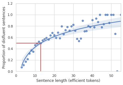
While people generally don’t even notice disfluencies in day-to-day conversation, early foundational work in computational linguistics demonstrated how common they are. In 1994, using the Switchboard corpus, Elizabeh Shriberg demonstrated that there is a 50% probability for a sentence of 10–13 words to include a disfluency and that the probability increases with sentence length.

The proportion of sentences from the Switchboard dataset with at least one disfluency plotted against sentence length measured in non-disfluent (i.e., efficient) tokens in the sentence. The longer a sentence gets, the more likely it is to contain a disfluency.

In “Teaching BERT to Wait: Balancing Accuracy and Latency for Streaming Disfluency Detection”, we present research findings on how to “clean up” transcripts of spoken text. We create more readable transcripts and captions of human speech by finding and removing disfluencies in people’s speech. Using labeled data, we created machine learning (ML) algorithms that identify disfluencies in human speech. Once those are identified we can remove the extra words to make transcripts more readable. This also improves the performance of natural language processing (NLP) algorithms that work on transcripts of human speech. Our work puts special priority on ensuring that these models are able to run on mobile devices so that we can protect user privacy and preserve performance in scenarios with low connectivity.

Base Model Overview
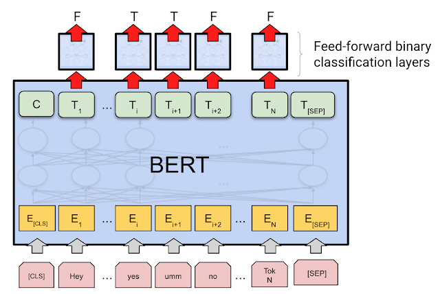
At the core of our base model is a pre-trained BERTBASE encoder with 108.9 million parameters. We use the standard per-token classifier configuration, with a binary classification head being fed by the sequence encodings for each token.

Illustration of how tokens in text become numerical embeddings, which then lead to output labels.

<!–

Illustration of how tokens in text become numerical embeddings, which then lead to output labels.

–>

We refined the BERT encoder by continuing the pretraining on the comments from the Pushrift Reddit dataset from 2019. Reddit comments are not speech data, but are more informal and conversational than the wiki and book data. This trains the encoder to better understand informal language, but may run the risk of internalizing some of the biases inherent in the data. For our particular use case, however, the model only captures the syntax or overall form of the text, not its content, which avoids potential issues related to semantic-level biases in the data.

We fine-tune our model for disfluency classification on hand-labeled corpora, such as the Switchboard corpus mentioned above. Hyperparameters (batch size, learning rate, number of training epochs, etc.) were optimized using Vizier.

We also produce a range of “small” models for use on mobile devices using a knowledge distillation technique known as “self training”. Our best small model is based on the Small-vocab BERT variant with 3.1 million parameters. This smaller model achieves comparable results to our baseline at 1% the size (in MiB). You can read more about how we achieved this model miniaturization in our 2021 Interspeech paper.

Streaming
Some of the latest use cases for automatic speech transcription include automated live captioning, such as produced by the Android “Live Captions” feature, which automatically transcribes spoken language in audio being played on the device. For disfluency removal to be of use in improving the readability of the captions in this setting, then it must happen quickly and in a stable manner. That is, the model should not change its past predictions as it sees new words in the transcript.

We call this live token-by-token processing streaming. Accurate streaming is difficult because of temporal dependencies; most disfluencies are only recognizable later. For example, a repetition does not actually become a repetition until the second time the word or phrase is said.

To investigate whether our disfluency detection model is effective in streaming applications, we split the utterances in our training set into prefix segments, where only the first N tokens of the utterance were provided at training time, for all values of N up to the full length of the utterance. We evaluated the model simulating a stream of spoken text by feeding prefixes to the models and measuring the performance with several metrics that capture model accuracy, stability, and latency including streaming F1, time to detection (TTD), edit overhead (EO), and average wait time (AWT). We experimented with look-ahead windows of either one or two tokens, allowing the model to “peek” ahead at additional tokens for which the model is not required to produce a prediction. In essence, we’re asking the model to “wait” for one or two more tokens of evidence before making a decision.

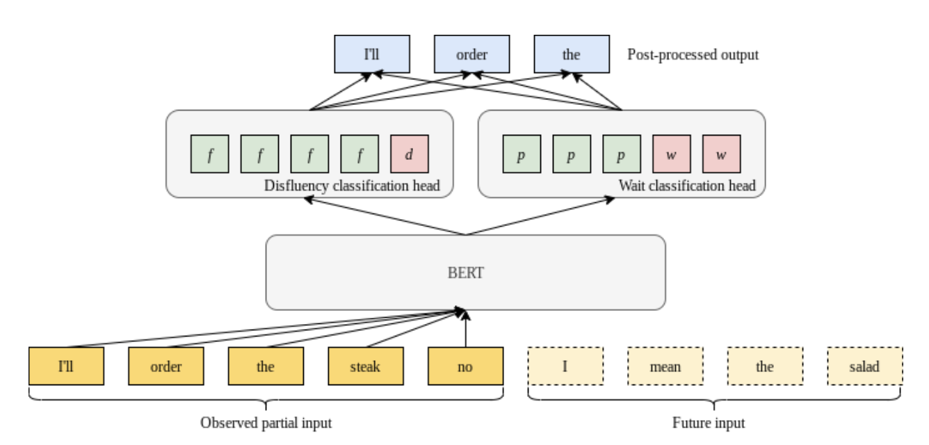
While adding this fixed look-ahead did improve the stability and streaming F1 scores in many contexts, we found that in some cases the label was already clear even without looking ahead to the next token and the model did not necessarily benefit from waiting. Other times, waiting for just one extra token was sufficient. We hypothesized that the model itself could learn when it should wait for more context. Our solution was a modified model architecture that includes a “wait” classification head that decides when the model has seen enough evidence to trust the disfluency classification head.
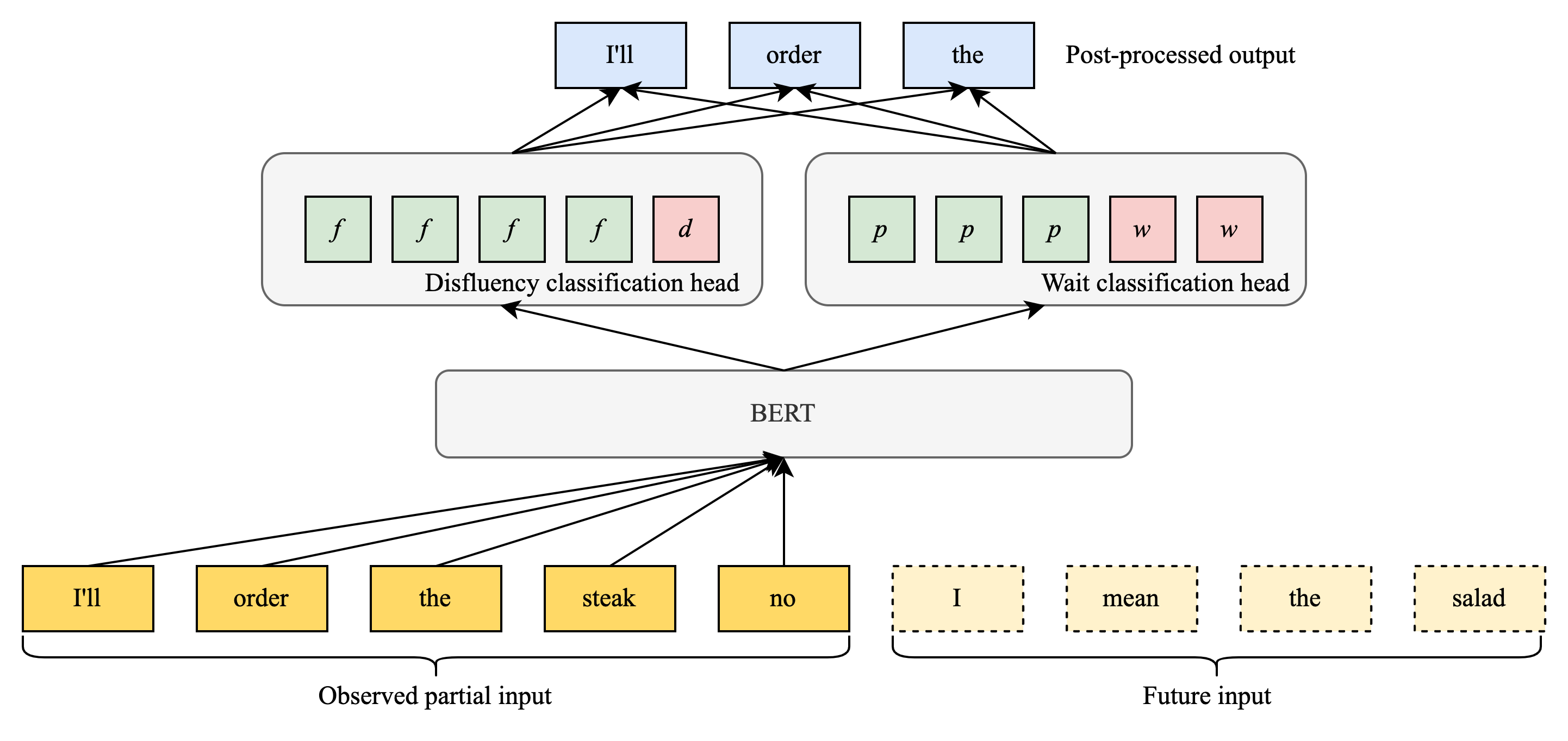
Diagram showing how the model labels input tokens as they arrive. The BERT embedding layers feed into two separate classification heads, which are combined for the output.

<!–

Diagram showing how the model labels input tokens as they arrive. The BERT embedding layers feed into two separate classification heads, which are combined for the output.

–>

We constructed a training loss function that is a weighted sum of three factors:

  1. The traditional cross-entropy loss for the disfluency classification head
  2. A cross-entropy term that only considers up to the first token with a “wait” classification
  3. A latency penalty that discourages the model from waiting too long to make a prediction

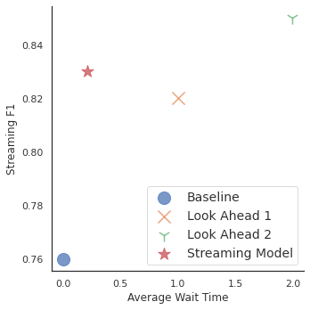
We evaluated this streaming model as well as the standard baseline with no look-ahead and with both 1- and 2-token look-ahead values:

Graph of the streaming F1 score versus the average wait time in tokens. Three data points indicate F1 scores above 0.82 across multiple wait times. The proposed streaming model achieves near top performance with much shorter wait times than the fixed look ahead models.

The streaming model achieved a better streaming F1 score than both a standard baseline with no look ahead and a model with a look ahead of 1. It performed nearly as well as the variant with fixed look ahead of 2, but with much less waiting. On average the model waited for only 0.21 tokens of context.

Internationalization
Our best outcomes so far have been with English transcripts. This is mostly due to resourcing issues: while there are a number of relatively large labeled conversational datasets that include disfluencies in English, other languages often have very few such datasets available. So, in order to make disfluency detection models available outside English a method is needed to build models in a way that does not require finding and labeling hundreds of thousands of utterances in each target language. A promising solution is to leverage multi-language versions of BERT to transfer what a model has learned about English disfluencies to other languages in order to achieve similar performance with much less data. This is an area of active research, but we do have some promising results to outline here.

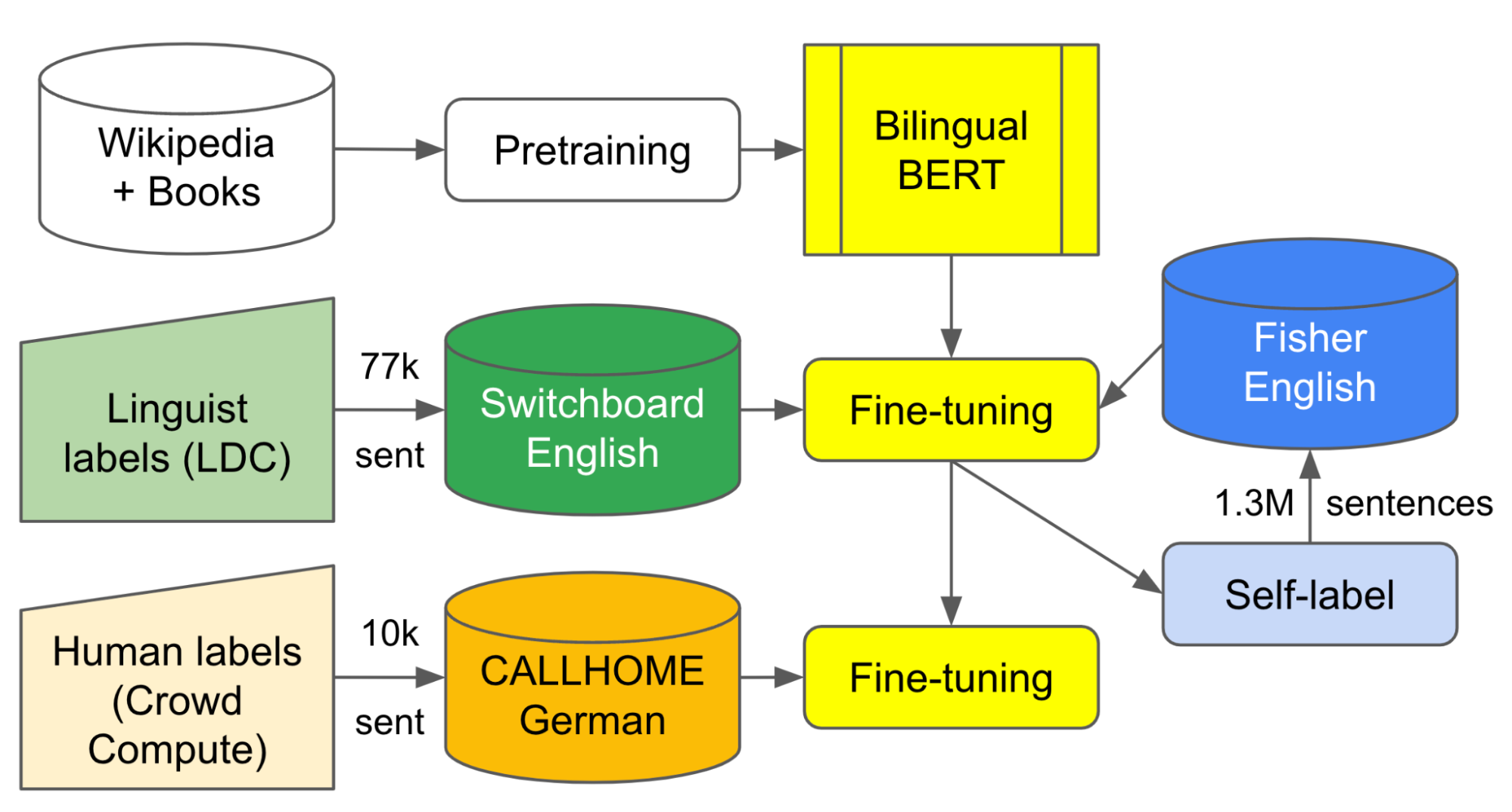
As a first effort to validate this approach, we added labels to about 10,000 lines of dialogue from the German CALLHOME dataset. We then started with the Geotrend English and German Bilingual BERT model (extracted from Multilingual BERT) and fine-tuned it with approximately 77,000 disfluency-labeled English Switchboard examples and 1.3 million examples of self-labeled transcripts from the Fisher Corpus. Then, we did further fine tuning with about 7,500 in-house–labeled examples from the German CALLHOME dataset.

Diagram illustrating the flow of labeled data and self-trained output in our best multilingual training setup. By training on both English and German data we are able to improve performance via transfer learning.

Our results indicate that fine-tuning on a large English corpus can produce acceptable precision using zero-shot transfer to similar languages like German, but at least a modest amount of German labels were needed to improve recall from less than 60% to greater than 80%. Two-stage fine-tuning of an English-German bilingual model produced the highest precision and overall F1 score.

Approach Precision Recall F1
German BERTBASE model fine-tuned on 7,300 human-labeled German CALLHOME examples 89.1% 81.3% 85.0
Same as above but with additional 7,500 self-labeled German CALLHOME examples 91.5% 83.3% 87.2
English/German Bilingual BERTbase model fine-tuned on English Switchboard+Fisher, evaluated on German CALLHOME (zero-shot language transfer) 87.2% 59.1% 70.4
Same as above but subsequently fine-tuned with 14,800 German CALLHOME (human- and self-labeled) examples 95.5% 82.6% 88.6

Conclusion
Cleaning up disfluencies from transcripts can improve not just their readability for people, but also the performance of other models that consume transcripts. We demonstrate effective methods for identifying disfluencies and expand our disfluency model to resource-constrained environments, new languages, and more interactive use cases.

Acknowledgements
Thank you to Vicky Zayats, Johann Rocholl, Angelica Chen, Noah Murad, Dirk Padfield, and Preeti Mohan for writing the code, running the experiments, and composing the papers discussed here. Wealso thank our technical product manager Aaron Schneider, Bobby Tran from the Cerebra Data Ops team, and Chetan Gupta from Speech Data Ops for their support obtaining additional data labels.

Read More

Minerva: Solving Quantitative Reasoning Problems with Language Models

Language models have demonstrated remarkable performance on a variety of natural language tasks — indeed, a general lesson from many works, including BERT, GPT-3, Gopher, and PaLM, has been that neural networks trained on diverse data at large scale in an unsupervised way can perform well on a variety of tasks.

Quantitative reasoning is one area in which language models still fall far short of human-level performance. Solving mathematical and scientific questions requires a combination of skills, including correctly parsing a question with natural language and mathematical notation, recalling relevant formulas and constants, and generating step-by-step solutions involving numerical calculations and symbolic manipulation. Due to these challenges, it is often believed that solving quantitative reasoning problems using machine learning will require significant advancements in model architecture and training techniques, granting models access to external tools such as Python interpreters, or possibly a more profound paradigm shift.

In “Solving Quantitative Reasoning Problems With Language Models” (to be released soon on the arXiv), we present Minerva, a language model capable of solving mathematical and scientific questions using step-by-step reasoning. We show that by focusing on collecting training data that is relevant for quantitative reasoning problems, training models at scale, and employing best-in-class inference techniques, we achieve significant performance gains on a variety of difficult quantitative reasoning tasks. Minerva solves such problems by generating solutions that include numerical calculations and symbolic manipulation without relying on external tools such as a calculator. The model parses and answers mathematical questions using a mix of natural language and mathematical notation. Minerva combines several techniques, including few-shot prompting, chain of thought or scratchpad prompting, and majority voting, to achieve state-of-the-art performance on STEM reasoning tasks. You can explore Minerva’s output with our interactive sample explorer!

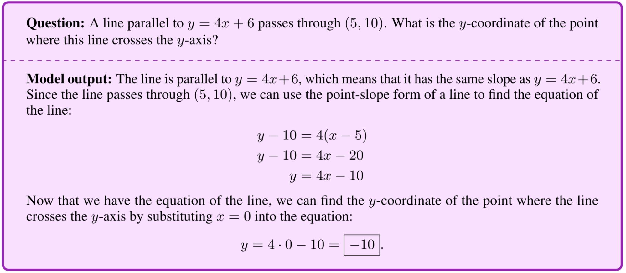
Solving a multi-step problem: A question from the MATH dataset and Minerva’s solution. The model writes down a line equation, simplifies it, substitutes a variable, and solves for y.

A Model Built for Multi-step Quantitative Reasoning
To promote quantitative reasoning, Minerva builds on the Pathways Language Model (PaLM), with further training on a 118GB dataset of scientific papers from the arXiv preprint server and web pages that contain mathematical expressions using LaTeX, MathJax, or other mathematical typesetting formats. Standard text cleaning procedures often remove symbols and formatting that are essential to the semantic meaning of mathematical expressions. By maintaining this information in the training data, the model learns to converse using standard mathematical notation.

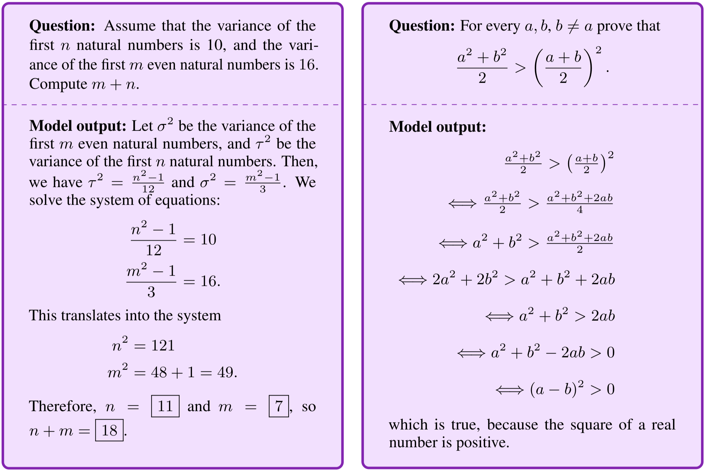
Example questions from the Joint Entrance Examination Main Math 2020 exam taken each year by almost 2M Indian high-school students intended to study engineering and similar fields (left), and the National Math Exam in Poland (May 2022) taken by approximately 270K high-school students every year (right).
A dataset for quantitative reasoning: Careful data processing preserves mathematical information, allowing the model to learn mathematics at a higher level.

Minerva also incorporates recent prompting and evaluation techniques to better solve mathematical questions. These include chain of thought or scratchpad prompting — where Minerva is prompted with several step-by-step solutions to existing questions before being presented with a new question — and majority voting. Like most language models, Minerva assigns probabilities to different possible outputs. When answering a question, rather than taking the single solution Minerva scores as most likely, multiple solutions are generated by sampling stochastically from all possible outputs. These solutions are different (e.g., the steps are not identical), but often arrive at the same final answer. Minerva uses majority voting on these sampled solutions, taking the most common result as the conclusive final answer.

Majority voting: Minerva generates multiple solutions to each question and chooses the most common answer as the solution, improving performance significantly.

Evaluation on STEM Benchmarks
To test Minerva’s quantitative reasoning abilities we evaluated the model on STEM benchmarks ranging in difficulty from grade school level problems to graduate level coursework.

  • MATH: High school math competition level problems
  • MMLU-STEM: A subset of the Massive Multitask Language Understanding benchmark focused on STEM, covering topics such as engineering, chemistry, math, and physics at high school and college level.
  • GSM8k: Grade school level math problems involving basic arithmetic operations that should all be solvable by a talented middle school student.

We also evaluated Minerva on OCWCourses, a collection of college and graduate level problems covering a variety of STEM topics such as solid state chemistry, astronomy, differential equations, and special relativity that we collected from MIT OpenCourseWare.

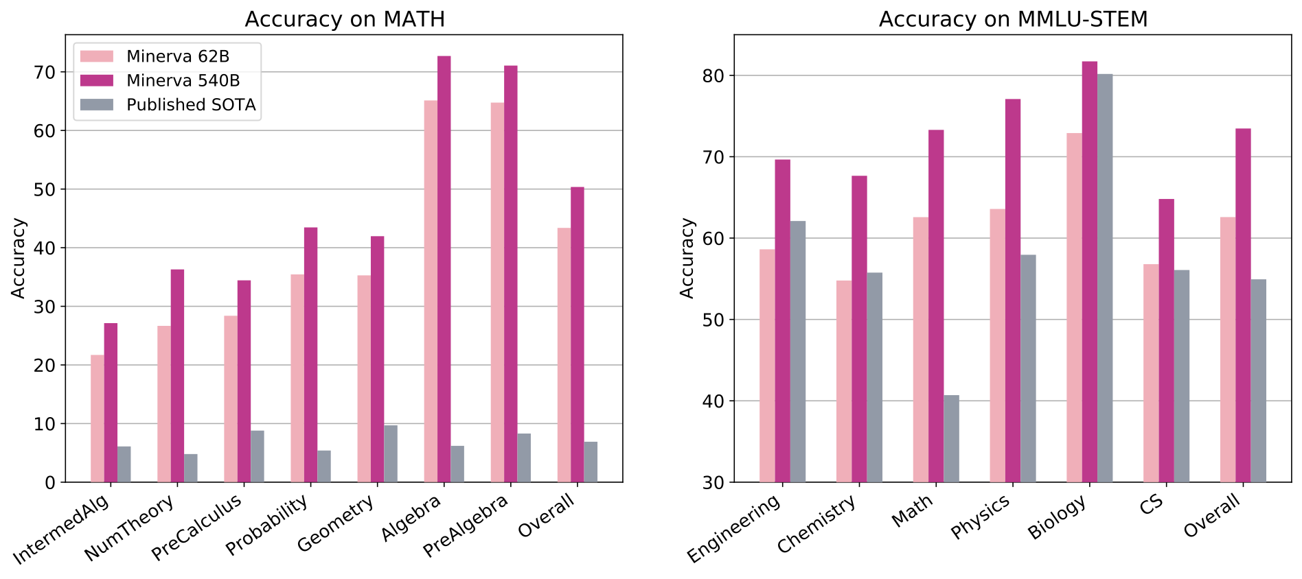
In all cases, Minerva obtains state-of-the-art results, sometimes by a wide margin.

Evaluation results on MATH and MMLU-STEM, which include high school and college level questions covering a range of STEM topics.
Model   MATH     MMLU-STEM     OCWCourses     GSM8k  
Minerva 50.3% 75% 30.8% 78.5%
Published state of the art    6.9% 55% 74.4%
Minerva 540B significantly improves state-of-the-art performance on STEM evaluation datasets.

What Minerva Gets Wrong
Minerva still makes its fair share of mistakes. To better identify areas where the model can be improved, we analyzed a sample of questions the model gets wrong, and found that most mistakes are easily interpretable. About half are calculation mistakes, and the other half are reasoning errors, where the solution steps do not follow a logical chain of thought.

It is also possible for the model to arrive at a correct final answer but with faulty reasoning. We call such cases “false positives”, as they erroneously count toward a model’s overall performance score. In our analysis, we find that the rate of false positives is relatively low (Minerva 62B produces less than 8% false positives on MATH).

Below are a couple of example mistakes the model makes.

Calculation mistake: The model incorrectly cancels the square root on both sides of the equation.
Reasoning mistake: The model computes the number of free throws at the fourth practice, but then uses this number as the final answer for the first practice.

Limitations
Our approach to quantitative reasoning is not grounded in formal mathematics. Minerva parses questions and generates answers using a mix of natural language and LaTeX mathematical expressions, with no explicit underlying mathematical structure. This approach has an important limitation, in that the model’s answers cannot be automatically verified. Even when the final answer is known and can be verified, the model can arrive at a correct final answer using incorrect reasoning steps, which cannot be automatically detected. This limitation is not present in formal methods for theorem proving (e.g., see Coq, Isabelle, HOL, Lean, Metamath, and Mizar). On the other hand, an advantage of the informal approach is that it can be applied to a highly diverse set of problems which may not lend themselves to formalization.

Future Directions
While machine learning models have become impressive tools in many scientific disciplines, they are often narrowly scoped to solve specific tasks. We hope that general models capable of solving quantitative reasoning problems will help push the frontiers of science and education. Models capable of quantitative reasoning have many potential applications, including serving as useful aids for researchers, and enabling new learning opportunities for students. We present Minerva as a small step in this direction. To see more samples from Minerva, such as the one below, please visit the interactive sample explorer!

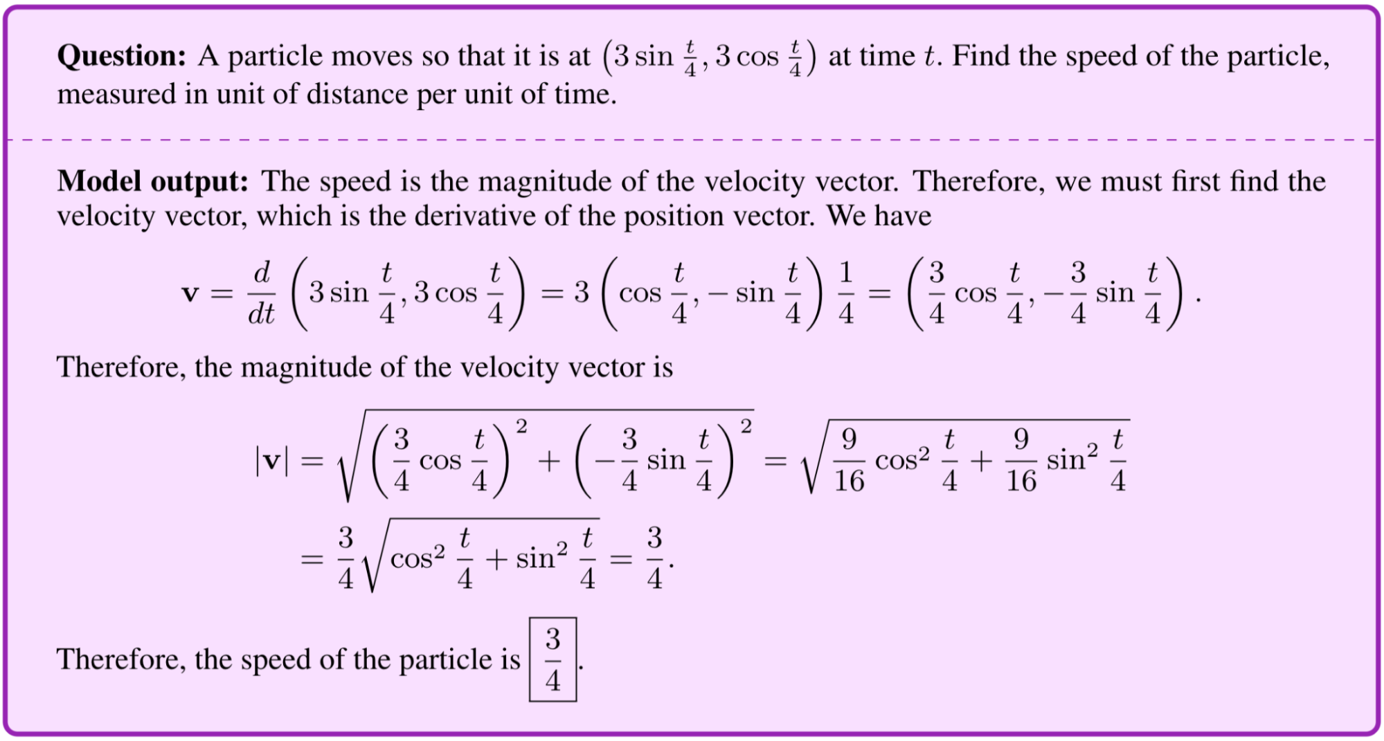
Solving a problem using calculus and trigonoometry: A question from the MATH dataset asking for the speed of a particle in circular motion. Minerva finds a correct step-by-step solution. In the process, Minerva computes a time derivative and applies a trigonometric identity.

Acknowledgements
Minerva was a collaborative effort that spanned multiple teams in Google Research. We would like to thank our coauthors Aitor Lewkowycz, Ambrose Slone, Anders Andreassen, Behnam Neyshabur, Cem Anil, David Dohan, Henryk Michalewski, Imanol Schlag, Theo Gutman-Solo, Vedant Misra, Vinay Ramasesh, and Yuhuai Wu, as well as our collaborators Erik Zelikman and Yasaman Razeghi. Minerva builds upon the work of many others at Google, and we would like to thank the PaLM team, the T5X team, the Flaxformer team, and the JAX team for their efforts. We thank Tom Small for designing the animation in this post. We would also like to especially thank Vedant Misra for developing the Minerva sample explorer.

Read More

Mahima Pushkarna is making data easier to understand

Five years ago, information designer Mahima Pushkarna joined Google to make data easier to understand. As a senior interaction designer on the People + AI Research (PAIR) team, she designed Data Cards to help everyone better understand the contexts of the data they are using. The Data Cards Playbook puts Google’s AI Principles into practice by providing opportunities for feedback, relevant explanations and appeal.

Recently, Mahima’s paper on Data Cards (co-written with Googlers Andrew Zaldivar and Oddur Kjartansson) was accepted to the ACM Conference on Fairness, Accountability and Transparency (ACM FAccT). Let’s catch up with her and find out more about what brought her to Google.

How did your background lead you to the work you’re doing now?

I’ve always been fascinated by conjuring up solutions to things. The kind of questions that I’ve found meaningful are those that are never truly solved, or never have one correct answer. (The kind of questions that exasperate us!) Those have been the problems I am always drawn towards.

Early in my career, I realized the power in visualizing data, but spreadsheets were intimidating. I wondered how design could make communicating complexity easier. So I found myself in grad school in Boston studying information design and data visualization. I focused on how people experience data and how our relationships to each other and our contexts are mediated.

I joined Google Brain as the first visual designer in a full-time capacity, though I had no background in artificial intelligence or machine learning — this was the deep end of the pool. This opened up the space to explore human-AI interaction, and make AI more accessible to a broader class of developers. At PAIR, my work focuses on making information experiences more meaningful for developers, researchers and others who build AI technologies.

What’s it like to have a unique background as a designer on a technical AI research team?

When you’re an engineer and immersed in building technology, it’s easy to assume everyone has a similar experience to your own — especially when you’re surrounded by peers who share your expertise. The actual user experience is very personal and varies drastically across users and contexts. That particular clarity is what designers bring to the table.

I’ve been able to engage my engineering and research colleagues with simple, people-centered questions right in the very beginning. How are people using an AI tool? What are they learning from it? Who else might be involved in the conversation? Do they have the proficiency we assume they have?

Pull quote: “Identifying what we don’t know about data is just as important as articulating what we do know.”

How did you begin designing Data Cards?

This project started when I was working on another visualization toolkit, Facets, to communicate the skews and imbalances within datasets to help machine learning practitioners make informed decisions. At the time, transparency was a moving target. Andrew, Tulsee Doshi and I started to proactively think about fairness in data, and saw a huge gap in the documentation of human decisions that dot a dataset’s lifecycle.

This “invisible” information shapes how we use data and the outcomes of models trained on them. For example, a model trained on a dataset that captures age in just two or three buckets will have very different outcomes compared to a dataset with ten buckets. The goal of Data Cards is to make both visible and invisible information about datasets available and simple to understand, so people from a variety of backgrounds can knowledgeably make decisions.

As we cover in our FAccT paper, Andrew and Oddur and I arrived at two insights. The first is that identifying what we don’t know about data is just as important as articulating what we do know. In capturing these nuances, it is possible to narrow those knowledge gaps before even collecting data. The second thing that surprised us was the sheer number of people involved in a dataset’s life cycle, and how fragile knowledge is. Context is easily lost in translation both between and within teams, across documents, emails, people and time.

Data Cards stand on the shoulders of giants, like Data Sheets (Gebru, et al.) and Model Cards (Mitchell et al.). We’ve been immensely lucky to have had the support of many original authors on these seminal papers that have paved our path to FAccT.

How do you hope the paper is used across the tech industry?

Imagine a world in which finding verifiable information about the motivations of a dataset’s creators or performance of a model is as easy as learning about the ethical beliefs of a celebrity or the rating of a movie. Our vision for Data Cards is that they become a cultural mainstay — invisible, but their absence would be missed by ML practitioners.

In this paper, we introduce frameworks that other teams can use in their work. Alongside that, we’ve open-sourced the Data Cards Playbook, so we’re trying to lower the barrier to access in every way possible.

Read More

Reducing gender-based harms in AI with Sunipa Dev

Natural language processing (NLP) is a form of artificial intelligence that teaches computer programs how to take in, interpret, and produce language from large data sets. For example, grammar checkers use NLP to come up with grammar suggestions that help people write grammatically correct phrases. But as Google’s AI Principles note, it’s sometimes necessary to have human intervention to identify risks of unfair bias.

Sunipa Dev is a research scientist at Google who focuses on Responsible AI. Some of her work focuses specifically on ways to evaluate unfair bias in NLP outcomes, reducing harms for people with queer and non-binary identities. Sunipa’s work was recently featured at a workshop at the ACM Fairness, Accountability, and Transparency (FAcct) conference in Seoul, Korea.

In our interview, she emphasizes that her work is achievable only through forging collaborative partnerships between researchers, engineers, and AI practitioners with everyday users and communities.

What inspired you to take on this career path?

While working on my PhD at the University of Utah, I explored research questions such as, “How do we evaluate NLP tech if they contain biases?” As language models evolved, our questions about potential harms did, too. During my postdoc work at UCLA, we ran a study to evaluate challenges in various language models by surveying respondents who identified as non-binary and had some experience with AI. With a focus on gender bias, our respondents helped us understand that experiences with language technologies cannot be understood in isolation. Rather, we must consider how these technologies intersect with systemic discrimination, erasure, and marginalization. For example, the harm of misgendering by a language technology can be compounded for trans, non-binary, and gender-diverse individuals who are already fighting against society to defend their identities. And when it’s in your personal space, like on your devices while emailing or texting, these small jabs can build up to larger psychological damage.

What is your current role at Google?

I am currently a Research Scientist at the Responsible AI – Human Centered Technology team. In my current role, I am working to build a better understanding of how to avoid unfair bias in AI language models across different cultures and geographies, aligned with Google’s AI Principles.

This is a challenge because language changes, and so do cultures and regional laws as we move from one place to another. This can all impact how people express themselves, what identities they choose and how they experience discrimination on a daily basis. Gender bias can manifest in entirely different ways in different parts of the world. In some of my ongoing work that focuses on a non-Western point of view, we are working with social scientists and NGOs in India while engaging with local communities. We are using the voices of many people who are living in a specific region and asking, “What are the biases prevalent in their society?”

What is gender bias in NLP?

Written text and training data for language technologies can lack representation or misrepresent different gender identities; this can reflect social biases. As a result, some NLP technologies can reinforce gender stereotypes and slurs, erase people’s gender identities, or have reduced quality of service for marginalized communities. What drives me in my work is my goal to make language technologies more inclusive and usable.

Why does this matter for AI?

Gender can be such an integral part of someone’s identity, and having that wrongly assumed by an AI system can be triggering, unfair, and harmful. We need to work towards systems and societies that do not encode unfair biases and harmful stereotypes in order to break out of the cycle of perpetuating harms of stereotyping, misgendering, and erasure.

How can people who are not researchers, engineers or AI practitioners engage in this work?

A very direct way is for people to report potential harms as bugs within products they use. People can also participate in open discussions in workshops, panels and town halls. These are all helpful ways to build inclusive AI.

I want to emphasize, however, that the onus can’t only be on the user. It’s also on the side of the researcher, engineer and AI practitioner. The goal is to create a continuous feedback loop between humans and machines, with real people stepping in to ensure the creation of more responsible AI. As AI practitioners, we need to work with the people we’re trying to serve and have users collaborate with us to tell us what we need to do better.

Read More

Quantum Advantage in Learning from Experiments

In efforts to learn about the quantum world, scientists face a big obstacle: their classical experience of the world. Whenever a quantum system is measured, the act of this measurement destroys the “quantumness” of the state. For example, if the quantum state is in a superposition of two locations, where it can seem to be in two places at the same time, once it is measured, it will randomly appear either ”here” or “there”, but not both. We only ever see the classical shadows cast by this strange quantum world.

A growing number of experiments are implementing machine learning (ML) algorithms to aid in analyzing data, but these have the same limitations as the people they aim to help: They can’t directly access and learn from quantum information. But what if there were a quantum machine learning algorithm that could directly interact with this quantum data?

In “Quantum Advantage in Learning from Experiments”, a collaboration with researchers at Caltech, Harvard, Berkeley, and Microsoft published in Science, we show that a quantum learning agent can perform exponentially better than a classical learning agent at many tasks. Using Google’s quantum computer, Sycamore, we demonstrate the tremendous advantage that a quantum machine learning (QML) algorithm has over the best possible classical algorithm. Unlike previous quantum advantage demonstrations, no advances in classical computing power could overcome this gap. This is the first demonstration of a provable exponential advantage in learning about quantum systems that is robust even on today’s noisy hardware.

Quantum Speedup
QML combines the best of both quantum computing and the lesser-known field of quantum sensing.

Quantum computers will likely offer exponential improvements over classical systems for certain problems, but to realize their potential, researchers first need to scale up the number of qubits and to improve quantum error correction. What’s more, the exponential speed-up over classical algorithms promised by quantum computers relies on a big, unproven assumption about so-called “complexity classes” of problems — namely, that the class of problems that can be solved on a quantum computer is larger than those that can be solved on a classical computer.. It seems like a reasonable assumption, and yet, no one has proven it. Until it’s proven, every claim of quantum advantage will come with an asterisk: that it can do better than any known classical algorithm.

Quantum sensors, on the other hand, are already being used for some high-precision measurements and offer modest (and proven) advantages over classical sensors. Some quantum sensors work by exploiting quantum correlations between particles to extract more information about a system than it otherwise could have. For example, scientists can use a collection of N atoms to measure aspects of the atoms’ environment like the surrounding magnetic fields. Typically the sensitivity to the field that the atoms can measure scales with the square root of N. But if one uses quantum entanglement to create a complex web of correlations between the atoms, then one can improve the scaling to be proportional to N. But as with most quantum sensing protocols, this quadratic speed-up over classical sensors is the best one can ever do.

Enter QML, a technology that straddles the line between quantum computers and quantum sensors. QML algorithms make computations that are aided by quantum data. Instead of measuring the quantum state, a quantum computer can store quantum data and implement a QML algorithm to process the data without collapsing it. And when this data is limited, a QML algorithm can squeeze exponentially more information out of each piece it receives when considering particular tasks.

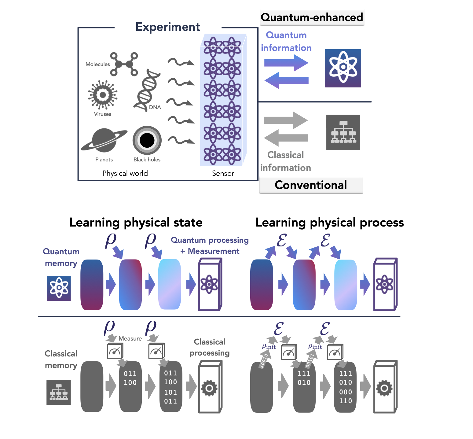
Comparison of a classical machine learning algorithm and a quantum machine learning algorithm. The classical machine learning algorithm measures a quantum system, then performs classical computations on the classical data it acquires to learn about the system. The quantum machine learning algorithm, on the other hand, interacts with the quantum states produced by the system, giving it a quantum advantage over the CML.

To see how a QML algorithm works, it’s useful to contrast with a standard quantum experiment. If a scientist wants to learn about a quantum system, they might send in a quantum probe, such as an atom or other quantum object whose state is sensitive to the system of interest, let it interact with the system, then measure the probe. They can then design new experiments or make predictions based on the outcome of the measurements. Classical machine learning (CML) algorithms follow the same process using an ML model, but the operating principle is the same — it’s a classical device processing classical information.

A QML algorithm instead uses an artificial “quantum learner.” After the quantum learner sends in a probe to interact with the system, it can choose to store the quantum state rather than measure it. Herein lies the power of QML. It can collect multiple copies of these quantum probes, then entangle them to learn more about the system faster.

Suppose, for example, the system of interest produces a quantum superposition state probabilistically by sampling from some distribution of possible states. Each state is composed of n quantum bits, or qubits, where each is a superposition of “0” and “1” — all learners are allowed to know the generic form of the state, but must learn its details.

In a standard experiment, where only classical data is accessible, every measurement provides a snapshot of the distribution of quantum states, but since it’s only a sample, it is necessary to measure many copies of the state to reconstruct it. In fact, it will take on the order of 2n copies.

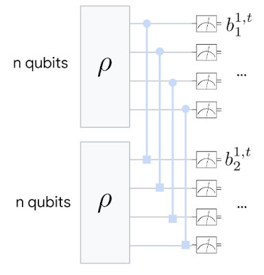
A QML agent is more clever. By saving a copy of the n-qubit state, then entangling it with the next copy that comes along, it can learn about the global quantum state more quickly, giving a better idea of what the state looks like sooner.

Basic schematic of the QML algorithm. Two copies of a quantum state are saved, then a “Bell measurement” is performed, where each pair is entangled and their correlations measured.

<!–

Basic schematic of the QML algorithm. Two copies of a quantum state are saved, then a “Bell measurement” is performed, where each pair is entangled and their correlations measured.

–>

The classical reconstruction is like trying to find an image hiding in a sea of noisy pixels — it could take a very long time to average-out all the noise to know what the image is representing. The quantum reconstruction, on the other hand, uses quantum mechanics to isolate the true image faster by looking for correlations between two different images at once.

Results
To better understand the power of QML, we first looked at three different learning tasks and theoretically proved that in each case, the quantum learning agent would do exponentially better than the classical learning agent. Each task was related to the example given above:

  1. Learning about incompatible observables of the quantum state — i.e., observables that cannot be simultaneously known to arbitrary precision due to the Heisenberg uncertainty principle, like position and momentum. But we showed that this limit can be overcome by entangling multiple copies of a state.
  2. Learning about the dominant components of the quantum state. When noise is present, it can disturb the quantum state. But typically the “principal component” — the part of the superposition with the highest probability — is robust to this noise, so we can still glean information about the original state by finding this dominant part.
  3. Learning about a physical process that acts on a quantum system or probe. Sometimes the state itself is not the object of interest, but a physical process that evolves this state is. We can learn about various fields and interactions by analyzing the evolution of a state over time.

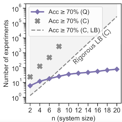
In addition to the theoretical work, we ran some proof-of-principle experiments on the Sycamore quantum processor. We started by implementing a QML algorithm to perform the first task. We fed an unknown quantum mixed state to the algorithm, then asked which of two observables of the state was larger. After training the neural network with simulation data, we found that the quantum learning agent needed exponentially fewer experiments to reach a prediction accuracy of 70% — equating to 10,000 times fewer measurements when the system size was 20 qubits. The total number of qubits used was 40 since two copies were stored at once.

Experimental comparison of QML vs. CML algorithms for predicting a quantum state’s observables. While the number of experiments needed to achieve 70% accuracy with a CML algorithm (“C” above) grows exponentially with the size of the quantum state n, the number of experiments the QML algorithm (“Q”) needs is only linear in n. The dashed line labeled “Rigorous LB (C)” represents the theoretical lower bound (LB) — the best possible performance — of a classical machine learning algorithm.

<!–

Experimental comparison of QML vs. CML algorithms for predicting a quantum state’s observables. While the number of experiments needed to achieve 70% accuracy with a CML algorithm (“C” above) grows exponentially with the size of the quantum state n, the number of experiments the QML algorithm (“Q”) needs is only linear in n. The dashed line labeled “Rigorous LB (C)” represents the theoretical lower bound (LB) — the best possible performance — of a classical machine learning algorithm.

–>

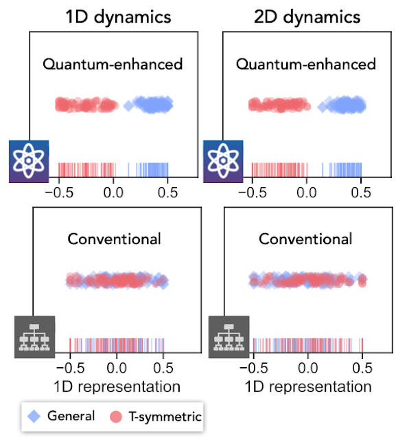
In a second experiment, relating to the task 3 above, we had the algorithm learn about the symmetry of an operator that evolves the quantum state of their qubits. In particular, if a quantum state might undergo evolution that is either totally random or random but also time-reversal symmetric, it can be difficult for a classical learner to tell the difference. In this task, the QML algorithm can separate the operators into two distinct categories, representing two different symmetry classes, while the CML algorithm fails outright. The QML algorithm was completely unsupervised, so this gives us hope that the approach could be used to discover new phenomena without needing to know the right answer beforehand.

Experimental comparison of QML vs. CML algorithms for predicting the symmetry class of an operator. While QML successfully separates the two symmetry classes, the CML fails to accomplish the task.

Conclusion
This experimental work represents the first demonstrated exponential advantage in quantum machine learning. And, distinct from a computational advantage, when limiting the number of samples from the quantum state, this type of quantum learning advantage cannot be challenged, even by unlimited classical computing resources.

So far, the technique has only been used in a contrived, “proof-of-principle” experiment, where the quantum state is deliberately produced and the researchers pretend not to know what it is. To use these techniques to make quantum-enhanced measurements in a real experiment, we’ll first need to work on current quantum sensor technology and methods to faithfully transfer quantum states to a quantum computer. But the fact that today’s quantum computers can already process this information to squeeze out an exponential advantage in learning bodes well for the future of quantum machine learning.

Acknowledgements
We would like to thank our Quantum Science Communicator Katherine McCormick for writing this blog post. Images reprinted with permission from Huang et al., Science, Vol 376:1182 (2022).

Read More

Mapping Urban Trees Across North America with the Auto Arborist Dataset

Over four billion people live in cities around the globe, and while most people interact daily with others — at the grocery store, on public transit, at work — they may take for granted their frequent interactions with the diverse plants and animals that comprise fragile urban ecosystems. Trees in cities, called urban forests, provide critical benefits for public health and wellbeing and will prove integral to urban climate adaptation. They filter air and water, capture stormwater runoff, sequester atmospheric carbon dioxide, and limit erosion and drought. Shade from urban trees reduces energy-expensive cooling costs and mitigates urban heat islands. In the US alone, urban forests cover 127M acres and produce ecosystem services valued at $18 billion. But as the climate changes these ecosystems are increasingly under threat.

Census data is typically not comprehensive, covering a subset of public trees and not including those in parks.

Urban forest monitoring — measuring the size, health, and species distribution of trees in cities over time — allows researchers and policymakers to (1) quantify ecosystem services, including air quality improvement, carbon sequestration, and benefits to public health; (2) track damage from extreme weather events; and (3) target planting to improve robustness to climate change, disease and infestation.

However, many cities lack even basic data about the location and species of their trees. Collecting such data via a tree census is costly (a recent Los Angeles census cost $2 million and took 18 months) and thus is typically conducted only by cities with substantial resources. Further, lack of access to urban greenery is a key aspect of urban social inequality, including socioeconomic and racial inequality. Urban forest monitoring enables the quantification of this inequality and the pursuit of its improvement, a key aspect of the environmental justice movement. But machine learning could dramatically lower tree census costs using a combination of street-level and aerial imagery. Such an automated system could democratize access to urban forest monitoring, especially for under-resourced cities that are already disproportionately affected by climate change. While there have been prior efforts to develop automated urban tree species recognition from aerial or street-level imagery, a major limitation has been a lack of large-scale labeled datasets.

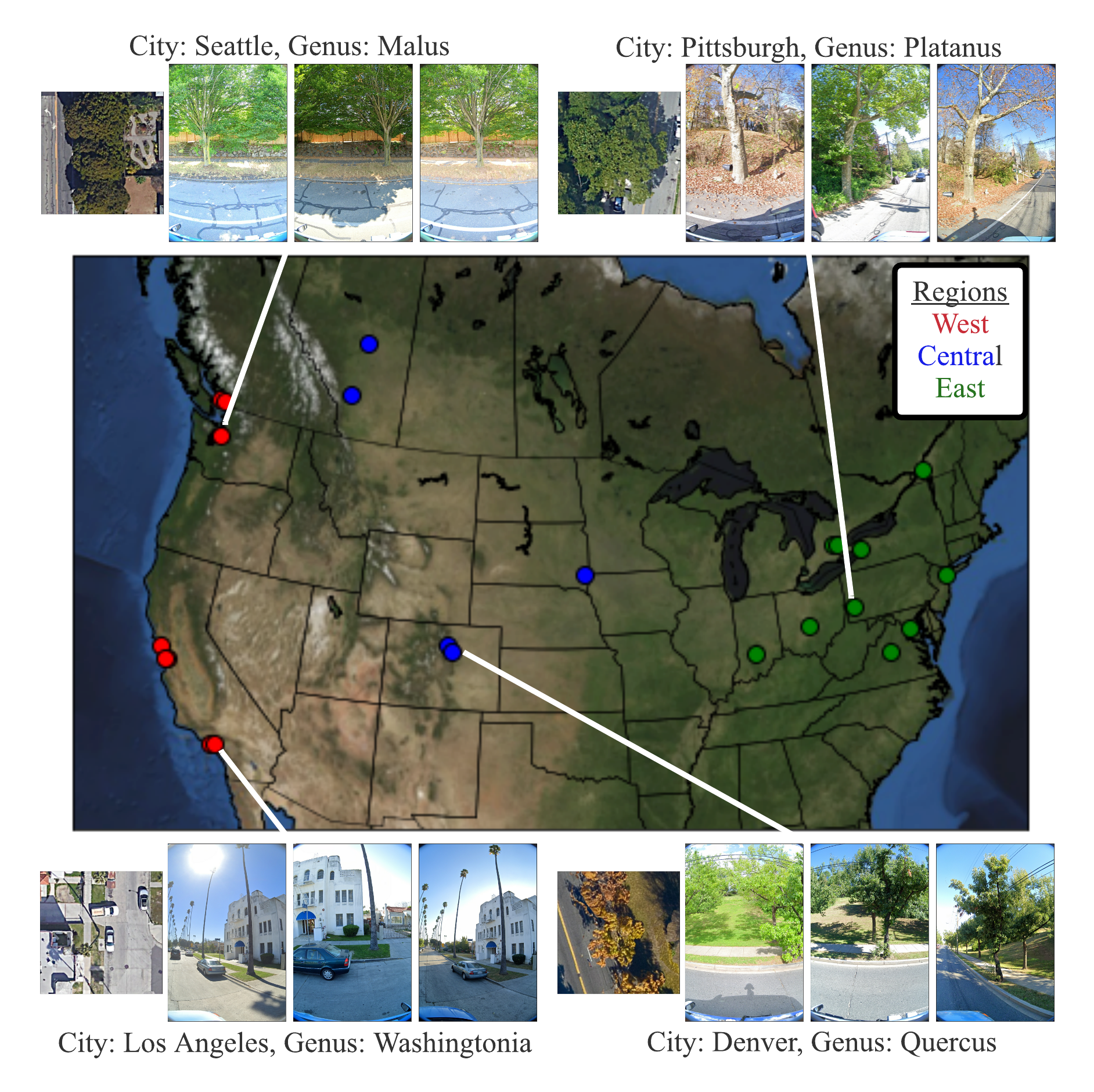
Today we introduce the Auto Arborist Dataset, a multiview urban tree classification dataset that, at ~2.6 million trees and >320 genera, is two orders of magnitude larger than those in prior work. To build the dataset, we pulled from public tree censuses from 23 North American cities (shown above) and merged these records with Street View and overhead RGB imagery. As the first urban forest dataset to cover multiple cities, we analyze in detail how forest models can generalize with respect to geographic distribution shifts, crucial to building systems that scale. We are releasing all 2.6M tree records publicly, along with aerial and ground-level imagery for 1M trees.

The 23 cities in the dataset are spread across North America, and are categorized into West, Central, and East regions to enable analysis of spatial and hierarchical generalization.
The number of tree records and genera in the dataset, per city and per region. The holdout city (which is never seen during training in any capacity) for each region is in bold.

The Auto Arborist Dataset
To curate Auto Arborist, we started from existing tree censuses which are provided by many cities online. For each tree census considered, we verified that the data contained GPS locations and genus/species labels, and was available for public use. We then parsed these data into a common format, fixing common data entry errors (such as flipped latitude/longitude) and mapping ground-truth genus names (and their common misspellings or alternate names) to a unified taxonomy. We have chosen to focus on genus prediction (instead of species-level prediction) as our primary task to avoid taxonomic complexity arising from hybrid and subspecies and the fact that there is more universal consensus on genus names than species names.

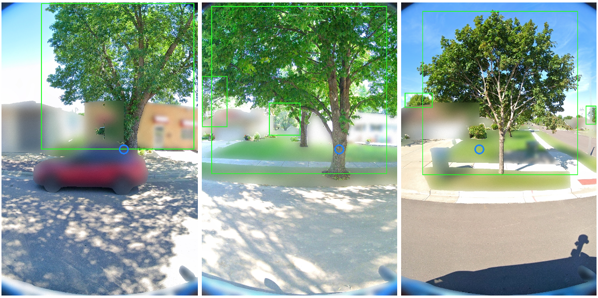
Next, using the provided geolocation for each tree, we queried an RGB aerial image centered on the tree and all street-level images taken within 2-10 meters around it. Finally, we filtered these images to (1) maximize our chances that the tree of interest is visible from each image and (2) preserve user privacy. This latter concern involved a number of steps including the removal of images that included people as determined by semantic segmentation and manual blurring, among others.

Selected Street View imagery from the Auto Arborist dataset. Green boxes represent tree detections (using a model trained on Open Images) and blue dots represent projected GPS location of the labeled tree.

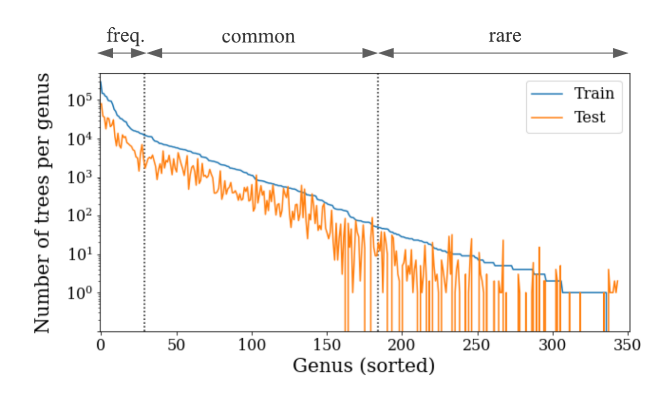
One of the most important challenges for urban forest monitoring is to do well in cities that were not part of the training set. Vision models must contend with distribution shifts, where the training distribution differs from the test distribution from a new city. Genus distributions vary geographically (e.g., there are more Douglas fir in western Canada than in California) and can also vary based on city size (LA is much larger than Santa Monica and contains many more genera). Another challenge is the long-tailed, fine-grained nature of tree genera, which can be difficult to disambiguate even for human experts, with many genera being quite rare.

The long-tailed distribution across Auto Arborist categories. Most examples come from a few frequent categories, and many categories have far fewer examples. We characterize each genus as frequent, common, or rare based on the number of training examples. Note that the test data is split spatially from the training data within each city, so not all rare genera are seen in the test set.

Finally, there are a number of ways in which tree images can have noise. For one, there is temporal variation in deciduous trees (for example, when aerial imagery includes leaves, but street-level images are bare). Moreover, public arboreal censuses are not always up-to-date. Thus, sometimes trees have died (and are no longer visible) in the time since the tree census was taken. In addition, aerial data quality can be poor (missing or obscured, e.g., by clouds).

Our curation process sought to minimize these issues by (1) only keeping images with sufficient tree pixels, as determined by a semantic segmentation model, (2) only keeping reasonably recent images, and (3) only keeping images where the tree position was sufficiently close to the street level camera. We considered also optimizing for trees seen in spring and summer, but decided seasonal variation could be a useful cue — we thus also released the date of each image to enable the community to explore the effects of seasonal variability.

Benchmark and Evaluation
To evaluate the dataset, we designed a benchmark to measure domain generalization and performance in the long tail of the distribution. We generated training and test splits at three levels. First, we split within each city (based on latitude or longitude) to see how well a city generalizes to itself. Second, we aggregate city-level training sets into three regions, West, Central, and East, holding out one city from each region. Finally, we merge the training sets across the three regions. For each of these splits, we report both accuracy and class-averaged recall for frequent, common and rare species on the corresponding held-out test sets.
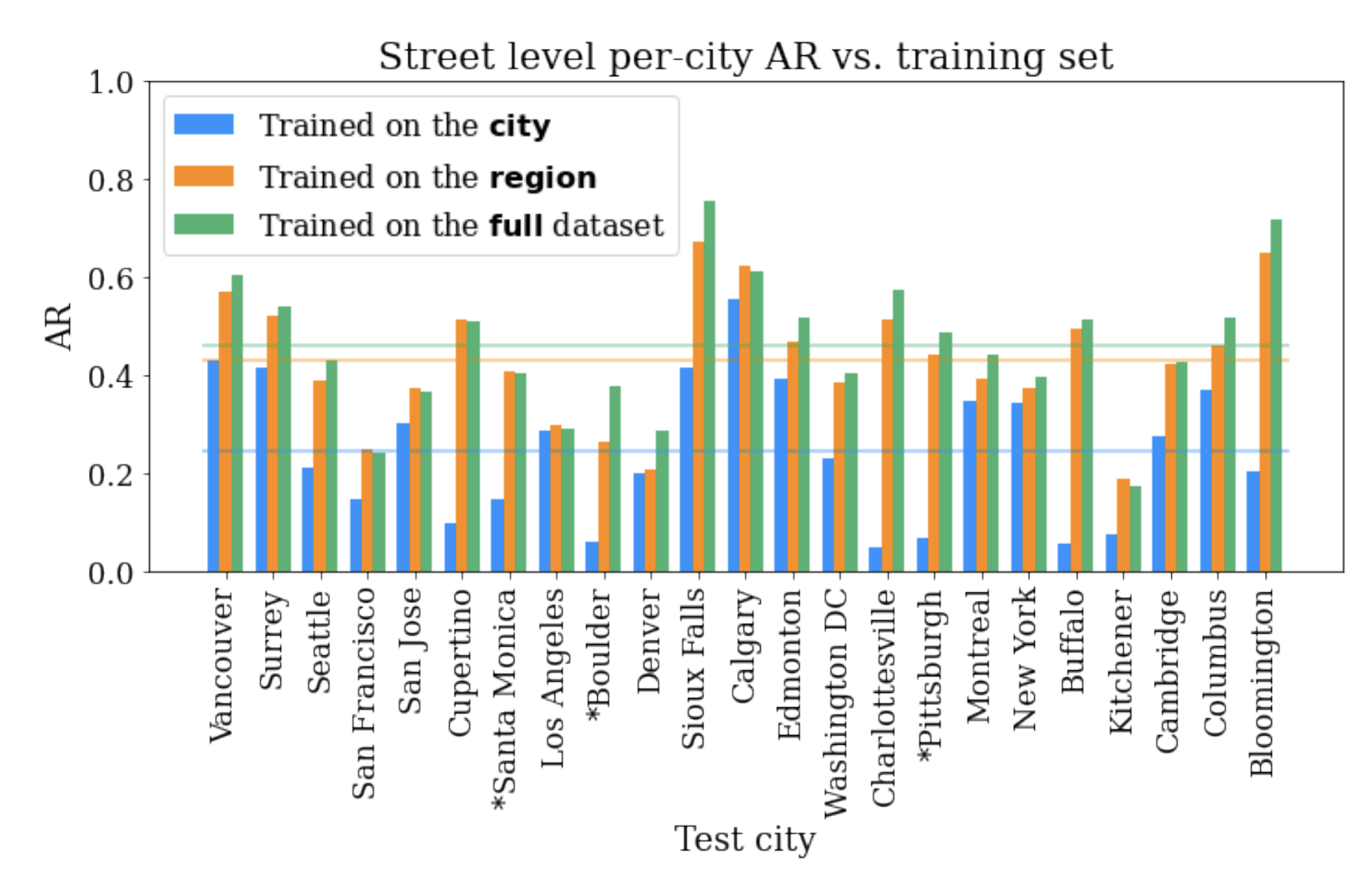
Using these metrics, we establish a performance baseline using standard modern convolutional models (ResNet). Our results demonstrate the benefits of a large-scale, geospatially distributed dataset such as Auto Arborist. First, we see that more training data helps — training on the entire dataset is better than training on a region, which is better than training on a single city.

The performance on each city’s test set when training on itself, on the region, and on the full training set.

Second, training on similar cities helps (and thus, having more coverage of cities helps). For example, if focusing on Seattle, then it is better to train on trees in Vancouver than Pittsburgh.

Cross-set performance, looking at the pairwise combination of train and test sets for each city. Note the block-diagonal structure, which highlights regional structure in the dataset.

Third, more data modalities and views help. The best performing models combine inputs from multiple Street View angles and overhead views. There remains much room for improvement, however, and this is where we believe the larger community of researchers can help.

Get Involved
By releasing the Auto Arborist Dataset, we step closer to the goal of affordable urban forest monitoring, enabling the computer vision community to tackle urban forest monitoring at scale for the first time. In the future, we hope to expand coverage to more North American cities (particularly in the South of the US and Mexico) and even worldwide. Further, we are excited to push the dataset to the more fine-grained species level and investigate more nuanced monitoring, including monitoring tree health and growth over time, and studying the effects of environmental factors on urban forests.

For more details, see our CVPR 2022 paper. This dataset is part of Google’s broader efforts to empower cities with data about urban forests, through the Environmental Insights Explorer Tree Canopy Lab and is available on our GitHub repo. If you represent a city that is interested in being included in the dataset please email auto-arborist+managers@googlegroups.com.

Acknowledgements
We would like to thank our co-authors Guanhang Wu, Trevor Edwards, Filip Pavetic, Bo Majewski, Shreyasee Mukherjee, Stanley Chan, John Morgan, Vivek Rathod, and Chris Bauer. We also thank Ruth Alcantara, Tanya Birch, and Dan Morris from Google AI for Nature and Society, John Quintero, Stafford Marquardt, Xiaoqi Yin, Puneet Lall, and Matt Manolides from Google Geo, Karan Gill, Tom Duerig, Abhijit Kundu, David Ross, Vighnesh Birodkar from Google Research (Perception team), and Pietro Perona for their support. This work was supported in part by the Resnick Sustainability Institute and was undertaken while Sara Beery was a Student Researcher at Google.

Read More

How AI creates photorealistic images from text

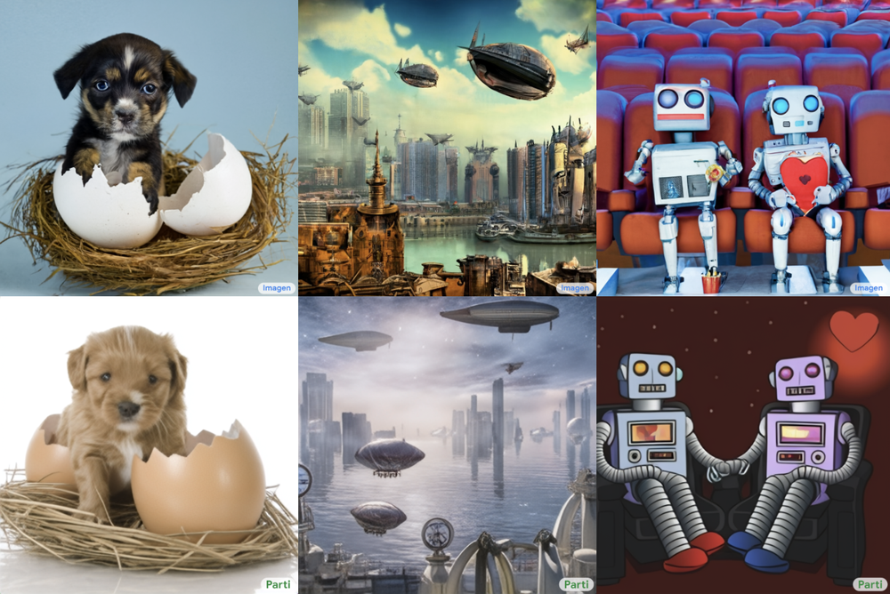
Pictures of puppy in a nest emerging from a cracked egg. Photos overlooking a steampunk city with airships. Picture of two robots having a romantic evening at the movies.

Have you ever seen a puppy in a nest emerging from a cracked egg? What about a photo that’s overlooking a steampunk city with airships? Or a picture of two robots having a romantic evening at the movies? These might sound far-fetched, but a novel type of machine learning technology called text-to-image generation makes them possible. These models can generate high-quality, photorealistic images from a simple text prompt.

Within Google Research, our scientists and engineers have been exploring text-to-image generation using a variety of AI techniques. After a lot of testing we recently announced two new text-to-image models — Imagen and Parti. Both have the ability to generate photorealistic images but use different approaches. We want to share a little more about how these models work and their potential.

How text-to-image models work

With text-to-image models, people provide a text description and the models produce images matching the description as closely as possible. This can be something as simple as “an apple” or “a cat sitting on a couch” to more complex details, interactions and descriptive indicators like “a cute sloth holding a small treasure chest. A bright golden glow is coming from the chest.”

A picture of a cute sloth holding a small treasure chest. A bright golden glow is coming from the chest

In the past few years, ML models have been trained on large image datasets with corresponding textual descriptions, resulting in higher quality images and a broader range of descriptions. This has sparked major breakthroughs in this area, including Open AI’s DALL-E 2.

How Imagen and Parti work

Imagen and Parti build on previous models. Transformer models are able to process words in relationship to one another in a sentence. They are foundational to how we represent text in our text-to-image models. Both models also use a new technique that helps generate images that more closely match the text description. While Imagen and Parti use similar technology, they pursue different, but complementary strategies.

Imagen is a Diffusion model, which learns to convert a pattern of random dots to images. These images first start as low resolution and then progressively increase in resolution. Recently, Diffusion models have seen success in both image and audio tasks like enhancing image resolution, recoloring black and white photos, editing regions of an image, uncropping images, and text-to-speech synthesis.

Parti’s approach first converts a collection of images into a sequence of code entries, similar to puzzle pieces. A given text prompt is then translated into these code entries and a new image is created. This approach takes advantage of existing research and infrastructure for large language models such as PaLM and is critical for handling long, complex text prompts and producing high-quality images.

These models have many limitations. For example, neither can reliably produce specific counts of objects (e.g. “ten apples”), nor place them correctly based on specific spatial descriptions (e.g. “a red sphere to the left of a blue block with a yellow triangle on it”). Also, as prompts become more complex, the models begin to falter, either missing details or introducing details that were not provided in the prompt. These behaviors are a result of several shortcomings, including lack of explicit training material, limited data representation, and lack of 3D awareness. We hope to address these gaps through broader representations and more effective integration into the text-to-image generation process.

Taking a responsible approach to Imagen and Parti

Text-to-image models are exciting tools for inspiration and creativity. They also come with risks related to disinformation, bias and safety. We’re having discussions around Responsible AI practices and the necessary steps to safely pursue this technology. As an initial step, we’re using easily identifiable watermarks to ensure people can always recognize an Imagen- or Parti-generated image. We’re also conducting experiments to better understand biases of the models, like how they represent people and cultures, while exploring possible mitigations. The Imagen and Parti papers provide extensive discussion of these issues.

What’s next for text-to-image models at Google

We will push on new ideas that combine the best of both models, and expand to related tasks such as adding the ability to interactively generate and edit images through text. We’re also continuing to conduct in-depth comparisons and evaluations to align with our Responsible AI Principles. Our goal is to bring user experiences based on these models to the world in a safe, responsible way that will inspire creativity.

Read More

Google at CVPR 2022

This week marks the beginning of the premier annual Computer Vision and Pattern Recognition conference (CVPR 2022), held both in-person in New Orleans, LA and virtually. As a leader in computer vision research and a Platinum Sponsor, Google will have a strong presence across CVPR 2022 with over 80 papers being presented at the main conference and active involvement in a number of conference workshops and tutorials.

If you are attending CVPR this year, please stop by our booth and chat with our researchers who are actively exploring the latest machine learning techniques for application to various areas of machine perception. Our researchers will also be available to talk about and demo several recent efforts, including on-device ML applications with MediaPipe, the Auto Arborist Dataset for urban forest monitoring, and much more.

You can also learn more about our research being presented at CVPR 2022 in the list below (Google affiliations in bold).

Organizing Committee

Tutorials Chairs
Include: Boqing Gong

Website Chairs
Include: AJ Piergiovanni

Area Chairs
Include: Alireza Fathi, Cordelia Schmid, Deqing Sun, Jonathan Barron, Michael Ryoo, Supasorn Suwajanakorn, Susanna Ricco

Diversity, Equity, and Inclusion Chairs
Include: Noah Snavely

Panel Discussion: Embodied Computer Vision
Panelists include: Michael Ryoo

Publications

Learning to Prompt for Continual Learning (see blog post)
Zifeng Wang*, Zizhao Zhang, Chen-Yu Lee, Han Zhang, Ruoxi Sun, Xiaoqi Ren, Guolong Su, Vincent Perot, Jennifer Dy, Tomas Pfister

GCR: Gradient Coreset Based Replay Buffer Selection for Continual Learning
Rishabh Tiwari, Krishnateja Killamsetty, Rishabh Iyer, Pradeep Shenoy

Zero-Shot Text-Guided Object Generation with Dream Fields
Ajay Jain, Ben Mildenhall, Jonathan T. Barron, Pieter Abbeel, Ben Poole

Towards End-to-End Unified Scene Text Detection and Layout Analysis
Shangbang Long, Siyang Qin, Dmitry Panteleev, Alessandro Bissacco, Yasuhisa Fujii, Michalis Raptis

FLOAT: Factorized Learning of Object Attributes for Improved Multi-object Multi-part Scene Parsing
Rishubh Singh, Pranav Gupta, Pradeep Shenoy, Ravikiran Sarvadevabhatla

LOLNerf: Learn from One Look
Daniel Rebain, Mark Matthews, Kwang Moo Yi, Dmitry Lagun, Andrea Tagliasacchi

Photorealistic Monocular 3D Reconstruction of Humans Wearing Clothing
Thiemo Alldieck, Mihai Zanfir, Cristian Sminchisescu

Learning Local Displacements for Point Cloud Completion
Yida Wang, David Joseph Tan, Nassir Navab, Federico Tombari

Density-Preserving Deep Point Cloud Compression
Yun He, Xinlin Ren, Danhang Tang, Yinda Zhang, Xiangyang Xue, Yanwei Fu

CMT-DeepLab: Clustering Mask Transformers for Panoptic Segmentation
Qihang Yu*, Huiyu Wang, Dahun Kim, Siyuan Qiao, Maxwell Collins, Yukun Zhu, Hartwig Adam, Alan Yuille, Liang-Chieh Chen

Deformable Sprites for Unsupervised Video Decomposition
Vickie Ye, Zhengqi Li, Richard Tucker, Angjoo Kanazawa, Noah Snavely

Learning with Neighbor Consistency for Noisy Labels
Ahmet Iscen, Jack Valmadre, Anurag Arnab, Cordelia Schmid

Multiview Transformers for Video Recognition
Shen Yan, Xuehan Xiong, Anurag Arnab, Zhichao Lu, Mi Zhang, Chen Sun, Cordelia Schmid

Kubric: A Scalable Dataset Generator
Klaus Greff, Francois Belletti, Lucas Beyer, Carl Doersch, Yilun Du, Daniel Duckworth, David J. Fleet, Dan Gnanapragasam, Florian Golemo, Charles Herrmann, Thomas Kipf, Abhijit Kundu, Dmitry Lagun, Issam Laradji, Hsueh-Ti (Derek) Liu, Henning Meyer, Yishu Miao, Derek Nowrouzezahrai, Cengiz Oztireli, Etienne Pot, Noha Radwan*, Daniel Rebain, Sara Sabour, Mehdi S. M. Sajjadi, Matan Sela, Vincent Sitzmann, Austin Stone, Deqing Sun, Suhani Vora, Ziyu Wang, Tianhao Wu, Kwang Moo Yi, Fangcheng Zhong, Andrea Tagliasacchi

3D Moments from Near-Duplicate Photos
Qianqian Wang, Zhengqi Li, David Salesin, Noah Snavely, Brian Curless, Janne Kontkanen

Mip-NeRF 360: Unbounded Anti-Aliased Neural Radiance Fields
Jonathan T. Barron, Ben Mildenhall, Dor Verbin, Pratul P. Srinivasan, Peter Hedman

RegNeRF: Regularizing Neural Radiance Fields for View Synthesis from Sparse Inputs
Michael Niemeyer*, Jonathan T. Barron, Ben Mildenhall, Mehdi S. M. Sajjadi, Andreas Geiger, Noha Radwan*

Ref-NeRF: Structured View-Dependent Appearance for Neural Radiance Fields
Dor Verbin, Peter Hedman, Ben Mildenhall, Todd Zickler, Jonathan T. Barron, Pratul P. Srinivasan

IRON: Inverse Rendering by Optimizing Neural SDFs and Materials from Photometric Images
Kai Zhang, Fujun Luan, Zhengqi Li, Noah Snavely

MAXIM: Multi-Axis MLP for Image Processing
Zhengzhong Tu*, Hossein Talebi, Han Zhang, Feng Yang, Peyman Milanfar, Alan Bovik, Yinxiao Li

Restormer: Efficient Transformer for High-Resolution Image Restoration
Syed Waqas Zamir, Aditya Arora, Salman Khan, Munawar Hayat, Fahad Shahbaz Khan, Ming-Hsuan Yang

Burst Image Restoration and Enhancement
Akshay Dudhane, Syed Waqas Zamir, Salman Khan, Fahad Shahbaz Khan, Ming-Hsuan Yang

Neural RGB-D Surface Reconstruction
Dejan Azinović, Ricardo Martin-Brualla, Dan B Goldman, Matthias Nießner, Justus Thies

Scene Representation Transformer: Geometry-Free Novel View Synthesis Through Set-Latent Scene Representations
Mehdi S. M. Sajjadi, Henning Meyer, Etienne Pot, Urs Bergmann, Klaus Greff, Noha Radwan*, Suhani Vora, Mario Lučić, Daniel Duckworth, Alexey Dosovitskiy*, Jakob Uszkoreit*, Thomas Funkhouser, Andrea Tagliasacchi*

ZebraPose: Coarse to Fine Surface Encoding for 6DoF Object Pose Estimation
Yongzhi Su, Mahdi Saleh, Torben Fetzer, Jason Rambach, Nassir Navab, Benjamin Busam, Didier Stricker, Federico Tombari

MetaPose: Fast 3D Pose from Multiple Views without 3D Supervision
Ben Usman, Andrea Tagliasacchi, Kate Saenko, Avneesh Sud

GPV-Pose: Category-Level Object Pose Estimation via Geometry-Guided Point-wise Voting
Yan Di, Ruida Zhang, Zhiqiang Lou, Fabian Manhardt, Xiangyang Ji, Nassir Navab, Federico Tombari

Rethinking Deep Face Restoration
Yang Zhao*, Yu-Chuan Su, Chun-Te Chu, Yandong Li, Marius Renn, Yukun Zhu, Changyou Chen, Xuhui Jia

Transferability Metrics for Selecting Source Model Ensembles
Andrea Agostinelli, Jasper Uijlings, Thomas Mensink, Vittorio Ferrari

Robust Fine-Tuning of Zero-Shot Models
Mitchell Wortsman, Gabriel Ilharco, Jong Wook Kim, Mike Li, Simon Kornblith, Rebecca Roelofs, Raphael Gontijo Lopes, Hannaneh Hajishirzi, Ali Farhadi, Hongseok Namkoong, Ludwig Schmidt

Block-NeRF: Scalable Large Scene Neural View Synthesis
Matthew Tancik, Vincent Casser, Xinchen Yan, Sabeek Pradhan, Ben Mildenhall, Pratul P. Srinivasan, Jonathan T. Barron, Henrik Kretzschmar

Light Field Neural Rendering
Mohammad Suhail*, Carlos Esteves, Leonid Sigal, Ameesh Makadia

Transferability Estimation Using Bhattacharyya Class Separability
Michal Pándy, Andrea Agostinelli, Jasper Uijlings, Vittorio Ferrari, Thomas Mensink

Matching Feature Sets for Few-Shot Image Classification
Arman Afrasiyabi, Hugo Larochelle, Jean-François Lalonde, Christian Gagné

Which Model to Transfer? Finding the Needle in the Growing Haystack
Cedric Renggli, André Susano Pinto, Luka Rimanic, Joan Puigcerver, Carlos Riquelme, Ce Zhang, Mario Lučić

Auditing Privacy Defenses in Federated Learning via Generative Gradient Leakage
Zhuohang Li, Jiaxin Zhang, Luyang Liu, Jian Liu

Estimating Example Difficulty Using Variance of Gradients
Chirag Agarwal, Daniel D’souza, Sara Hooker

More Than Words: In-the-Wild Visually-Driven Prosody for Text-to-Speech (see blog post)
Michael Hassid, Michelle Tadmor Ramanovich, Brendan Shillingford, Miaosen Wang, Ye Jia, Tal Remez

Robust Outlier Detection by De-Biasing VAE Likelihoods
Kushal Chauhan, Barath Mohan U, Pradeep Shenoy, Manish Gupta, Devarajan Sridharan

Deep 3D-to-2D Watermarking: Embedding Messages in 3D Meshes and Extracting Them from 2D Renderings
Innfarn Yoo, Huiwen Chang, Xiyang Luo, Ondrej Stava, Ce Liu*, Peyman Milanfar, Feng Yang

Knowledge Distillation: A Good Teacher Is Patient and Consistent
Lucas Beyer, Xiaohua Zhai, Amélie Royer*, Larisa Markeeva*, Rohan Anil, Alexander Kolesnikov

Urban Radiance Fields
Konstantinos Rematas, Andrew Liu, Pratul P. Srinivasan, Jonathan T. Barron, Andrea Tagliasacchi, Thomas Funkhouser, Vittorio Ferrari

Manifold Learning Benefits GANs
Yao Ni, Piotr Koniusz, Richard Hartley, Richard Nock

MaskGIT: Masked Generative Image Transformer
Huiwen Chang, Han Zhang, Lu Jiang, Ce Liu*, William T. Freeman

InOut: Diverse Image Outpainting via GAN Inversion
Yen-Chi Cheng, Chieh Hubert Lin, Hsin-Ying Lee, Jian Ren, Sergey Tulyakov, Ming-Hsuan Yang

Scaling Vision Transformers (see blog post)
Xiaohua Zhai, Alexander Kolesnikov, Neil Houlsby, Lucas Beyer

Fine-Tuning Image Transformers Using Learnable Memory
Mark Sandler, Andrey Zhmoginov, Max Vladymyrov, Andrew Jackson

PokeBNN: A Binary Pursuit of Lightweight Accuracy
Yichi Zhang*, Zhiru Zhang, Lukasz Lew

Bending Graphs: Hierarchical Shape Matching Using Gated Optimal Transport
Mahdi Saleh, Shun-Cheng Wu, Luca Cosmo, Nassir Navab, Benjamin Busam, Federico Tombari

Uncertainty-Aware Deep Multi-View Photometric Stereo
Berk Kaya, Suryansh Kumar, Carlos Oliveira, Vittorio Ferrari, Luc Van Gool

Depth-Supervised NeRF: Fewer Views and Faster Training for Free
Kangle Deng, Andrew Liu, Jun-Yan Zhu, Deva Ramanan

Dense Depth Priors for Neural Radiance Fields from Sparse Input Views
Barbara Roessle, Jonathan T. Barron, Ben Mildenhall, Pratul P. Srinivasan, Matthias Nießner

Trajectory Optimization for Physics-Based Reconstruction of 3D Human Pose from Monocular Video
Erik Gärtner, Mykhaylo Andriluka, Hongyi Xu, Cristian Sminchisescu

Differentiable Dynamics for Articulated 3D Human Motion Reconstruction
Erik Gärtner, Mykhaylo Andriluka, Erwin Coumans, Cristian Sminchisescu

Panoptic Neural Fields: A Semantic Object-Aware Neural Scene Representation
Abhijit Kundu, Kyle Genova, Xiaoqi Yin, Alireza Fathi, Caroline Pantofaru, Leonidas J. Guibas, Andrea Tagliasacchi, Frank Dellaert, Thomas Funkhouser

Pyramid Adversarial Training Improves ViT Performance
Charles Herrmann, Kyle Sargent, Lu Jiang, Ramin Zabih, Huiwen Chang, Ce Liu*, Dilip Krishnan, Deqing Sun

Proper Reuse of Image Classification Features Improves Object Detection
Cristina Vasconcelos, Vighnesh Birodkar, Vincent Dumoulin

SOMSI: Spherical Novel View Synthesis with Soft Occlusion Multi-Sphere Images
Tewodros Habtegebrial, Christiano Gava, Marcel Rogge, Didier Stricker, Varun Jampani

TubeFormer-DeepLab: Video Mask Transformer
Dahun Kim, Jun Xie, Huiyu Wang, Siyuan Qiao, Qihang Yu, Hong-Seok Kim, Hartwig Adam, In So Kweon, Liang-Chieh Chen

Contextualized Spatio-Temporal Contrastive Learning with Self-Supervision
Liangzhe Yuan, Rui Qian*, Yin Cui, Boqing Gong, Florian Schroff, Ming-Hsuan Yang, Hartwig Adam, Ting Liu

When Does Contrastive Visual Representation Learning Work?
Elijah Cole, Xuan Yang, Kimberly Wilber, Oisin Mac Aodha, Serge Belongie

Less Is More: Generating Grounded Navigation Instructions from Landmarks
Su Wang, Ceslee Montgomery, Jordi Orbay, Vighnesh Birodkar, Aleksandra Faust, Izzeddin Gur, Natasha Jaques, Austin Waters, Jason Baldridge, Peter Anderson

Forecasting Characteristic 3D Poses of Human Actions
Christian Diller, Thomas Funkhouser, Angela Dai

BEHAVE: Dataset and Method for Tracking Human Object Interactions
Bharat Lal Bhatnagar, Xianghui Xie, Ilya A. Petrov, Cristian Sminchisescu, Christian Theobalt, Gerard Pons-Moll

Motion-from-Blur: 3D Shape and Motion Estimation of Motion-Blurred Objects in Videos
Denys Rozumnyi, Martin R. Oswald, Vittorio Ferrari, Marc Pollefeys

End-to-End Generative Pretraining for Multimodal Video Captioning (see blog post)
Paul Hongsuck Seo, Arsha Nagrani, Anurag Arnab, Cordelia Schmid

Uncertainty-Aware Adaptation for Self-Supervised 3D Human Pose Estimation
Jogendra Nath Kundu, Siddharth Seth, Pradyumna YM, Varun Jampani, Anirban Chakraborty, R. Venkatesh Babu

Learning ABCs: Approximate Bijective Correspondence for Isolating Factors of Variation with Weak Supervision
Kieran A. Murphy, Varun Jampani, Srikumar Ramalingam, Ameesh Makadia

HumanNeRF: Free-Viewpoint Rendering of Moving People from Monocular Video
Chung-Yi Weng, Brian Curless, Pratul P. Srinivasan, Jonathan T. Barron, Ira Kemelmacher-Shlizerman

Deblurring via Stochastic Refinement
Jay Whang*, Mauricio Delbracio, Hossein Talebi, Chitwan Saharia, Alexandros G. Dimakis, Peyman Milanfar

NeRF in the Dark: High Dynamic Range View Synthesis from Noisy Raw Images
Ben Mildenhall, Peter Hedman, Ricardo Martin-Brualla, Pratul P. Srinivasan, Jonathan T. Barron

CoNeRF: Controllable Neural Radiance Fields
Kacper Kania, Kwang Moo Yi, Marek Kowalski, Tomasz Trzciński, Andrea Tagliasacchi

A Conservative Approach for Unbiased Learning on Unknown Biases
Myeongho Jeon, Daekyung Kim, Woochul Lee, Myungjoo Kang, Joonseok Lee

DeepFusion: Lidar-Camera Deep Fusion for Multi-Modal 3D Object Detection (see blog post)
Yingwei Li*, Adams Wei Yu, Tianjian Meng, Ben Caine, Jiquan Ngiam, Daiyi Peng, Junyang Shen, Yifeng Lu, Denny Zhou, Quoc V. Le, Alan Yuille, Mingxing Tan

Video Frame Interpolation Transformer
Zhihao Shi, Xiangyu Xu, Xiaohong Liu, Jun Chen, Ming-Hsuan Yang

Global Matching with Overlapping Attention for Optical Flow Estimation
Shiyu Zhao, Long Zhao, Zhixing Zhang, Enyu Zhou, Dimitris Metaxas

LiT: Zero-Shot Transfer with Locked-image Text Tuning (see blog post)
Xiaohua Zhai, Xiao Wang, Basil Mustafa, Andreas Steiner, Daniel Keysers, Alexander Kolesnikov, Lucas Beyer

Are Multimodal Transformers Robust to Missing Modality?
Mengmeng Ma, Jian Ren, Long Zhao, Davide Testuggine, Xi Peng

3D-VField: Adversarial Augmentation of Point Clouds for Domain Generalization in 3D Object Detection
Alexander Lehner, Stefano Gasperini, Alvaro Marcos-Ramiro, Michael Schmidt, Mohammad-Ali Nikouei Mahani, Nassir Navab, Benjamin Busam, Federico Tombari

SHIFT: A Synthetic Driving Dataset for Continuous Multi-Task Domain Adaptation
Tao Sun, Mattia Segu, Janis Postels, Yuxuan Wang, Luc Van Gool, Bernt Schiele, Federico Tombari, Fisher Yu

H4D: Human 4D Modeling by Learning Neural Compositional Representation
Boyan Jiang, Yinda Zhang, Xingkui Wei, Xiangyang Xue, Yanwei Fu

Gravitationally Lensed Black Hole Emission Tomography
Aviad Levis, Pratul P. Srinivasan, Andrew A. Chael, Ren Ng, Katherine L. Bouman

Deep Saliency Prior for Reducing Visual Distraction
Kfir Aberman, Junfeng He, Yossi Gandelsman, Inbar Mosseri, David E. Jacobs, Kai Kohlhoff, Yael Pritch, Michael Rubinstein

The Auto Arborist Dataset: A Large-Scale Benchmark for Multiview Urban Forest Monitoring Under Domain Shift
Sara Beery, Guanhang Wu, Trevor Edwards, Filip Pavetic, Bo Majewski, Shreyasee Mukherjee, Stanley Chan, John Morgan, Vivek Rathod, Jonathan Huang

Workshops

Ethical Considerations in Creative Applications of Computer Vision
Chairs and Advisors: Negar Rostamzadeh, Fernando Diaz, Emily Denton, Mark Diaz, Jason Baldridge

Dynamic Neural Networks Meet Computer Vision Organizers
Invited Speaker: Barret Zoph

Precognition: Seeing Through the Future
Organizer: Utsav Prabhu
Invited Speaker: Sella Nevo

Computer Vision in the Built Environment for the Design, Construction, and Operation of Buildings
Invited Speakers: Thomas Funkhouser, Federico Tombari

Neural Architecture Search: Lightweight NAS Challenge
Invited Speaker: Barret Zoph

Transformers in Vision
Organizer: Lucas Beyer
Invited Speakers and Panelists: Alexander Kolesnikov, Mathilde Caron, Arsha Nagrani, Lucas Beyer

Challenge on Learned Image Compression
Organizers: George Toderici, Johannes Balle, Eirikur Agustsson, Nick Johnston, Fabian Mentzer, Luca Versari
Invited Speaker: Debargha Mukherjee

Embodied AI
Organizers: Anthony Francis, Sören Pirk, Alex Ku, Fei Xia, Peter Anderson
Scientific Advisory Board Members: Alexander Toshev, Jie Tan
Invited Speaker: Carolina Parada

Sight and Sound
Organizers: Arsha Nagrani, William Freeman

New Trends in Image Restoration and Enhancement
Organizers: Ming-Hsuan Yang, Vivek Kwatra, George Toderici

EarthVision: Large Scale Computer Vision for Remote Sensing Imagery
Invited Speaker: John Quinn

LatinX in Computer Vision Research
Organizer: Ruben Villegas

Fine-Grained Visual Categorization
Organizer: Kimberly Wilber

The Art of Robustness: Devil and Angel in Adversarial Machine Learning
Organizer: Florian Tramèr
Invited Speaker: Nicholas Carlini

AI for Content Creation
Organizers: Deqing Sun, Huiwen Chang, Lu Jiang
Invited Speaker: Chitwan Saharia

LOng-form VidEo Understanding
Invited Speaker: Cordelia Schmid

Visual Perception and Learning in an Open World
Invited Speaker: Rahul Sukthankar

Media Forensics
Organizer : Christoph Bregler
Technical Committee Members: Shruti Agarwal, Scott McCloskey, Peng Zhou

Vision Datasets Understanding
Organizer: José Lezama

Embedded Vision
Invited Speaker: Matthias Grundmann

Federated Learning for Computer Vision
Invited Speaker: Zheng Xu

Large Scale Holistic Video Understanding
Organizer: David Ross
Invited Speaker: Anurag Arnab

Learning With Limited Labelled Data for Image and Video Understanding
Invited Speaker: Hugo Larochelle

Bridging the Gap Between Computational Photography and Visual Recognition
Invited Speaker: Xiaohua Zhai

Explainable Artificial Intelligence for Computer Vision
Invited Speaker: Been Kim

Robustness in Sequential Data
Organizers: Sayna Ebrahimi, Kevin Murphy
Invited Speakers: Sayna Ebrahimi, Balaji Lakshminarayanan

Sketch-Oriented Deep Learning
Organizer: David Ha
Invited Speaker: Jonas Jongejan

Multimodal Learning and Applications
Invited Speaker: Cordelia Schmid

Computational Cameras and Displays
Organizer: Tali Dekel
Invited Speaker: Peyman Millanfar

Artificial Social Intelligence
Invited Speaker: Natasha Jaques

VizWiz Grand Challenge: Algorithms to Assist People Who Are Blind
Invited Speaker and Panelist: Andrew Howard

Image Matching: Local Features & Beyond
Organizer: Eduard Trulls

Multi-Agent Behavior: Representation, Modeling, Measurement, and Applications
Organizer: Ting Liu

Efficient Deep Learning for Computer Vision
Organizers: Pete Warden, Andrew Howard, Grace Chu, Jaeyoun Kim

Gaze Estimation and Prediction in the Wild
Organizer: Thabo Beeler

Tutorials

Denoising Diffusion-Based Generative Modeling: Foundations and Applications
Invited Speaker: Ruiqi Gao

Algorithmic Fairness: Why It’s Hard and Why It’s Interesting
Invited Speaker: Sanmi Koyejo

Beyond Convolutional Neural Networks
Invited Speakers: Neil Houlsby, Alexander Kolesnikov, Xiaohua Zhai

Joint Ego4D and Egocentric Perception, Interaction & Computing
Invited Speaker: Vittorio Ferrari

Deep AUC Maximization
Invited Speakers: Tianbao Yang

Vision-Based Robot Learning
Organizers: Michael S. Ryoo, Andy Zeng, Pete Florence

Graph Machine Learning for Visual Computing
Organizers: Federico Tombari
Invited Speakers: Federico Tombari, Fabian Manhardt


*Work done while at Google.  

Read More

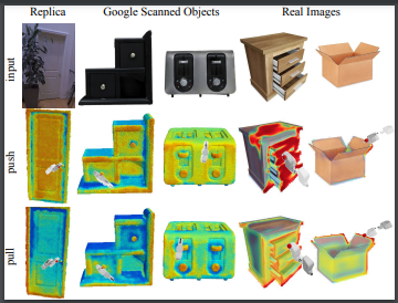
Scanned Objects by Google Research: A Dataset of 3D-Scanned Common Household Items

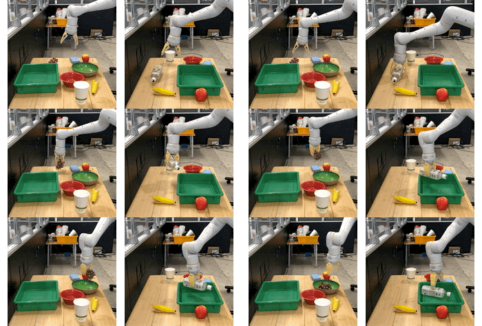
Many recent advances in computer vision and robotics rely on deep learning, but training deep learning models requires a wide variety of data to generalize to new scenarios. Historically, deep learning for computer vision has relied on datasets with millions of items that were gathered by web scraping, examples of which include ImageNet, Open Images, YouTube-8M, and COCO. However, the process of creating these datasets can be labor-intensive, and can still exhibit labeling errors that can distort the perception of progress. Furthermore, this strategy does not readily generalize to arbitrary three-dimensional shapes or real-world robotic data.

Real-world robotic data collection is very useful, but difficult to scale and challenging to label.

Simulating robots and environments using tools such as Gazebo, MuJoCo, and Unity can mitigate many of the inherent limitations in these datasets. However, simulation is only an approximation of reality — handcrafted models built from polygons and primitives often correspond poorly to real objects. Even if a scene is built directly from a 3D scan of a real environment, the movable objects in that scan will act like fixed background scenery and will not respond the way real-world objects would. Due to these challenges, there are few large libraries with high-quality models of 3D objects that can be incorporated into physical and visual simulations to provide the variety needed for deep learning.

In “Google Scanned Objects: A High-Quality Dataset of 3D Scanned Household Items”, presented at ICRA 2022, we describe our efforts to address this need by creating the Scanned Objects dataset, a curated collection of over 1000 3D-scanned common household items. The Scanned Objects dataset is usable in tools that read Simulation Description Format (SDF) models, including the Gazebo and PyBullet robotics simulators. Scanned Objects is hosted on Open Robotics, an open-source hosting environment for models compatible with the Gazebo simulator.

History
Robotics researchers within Google began scanning objects in 2011, creating high-fidelity 3D models of common household objects to help robots recognize and grasp things in their environments. However, it became apparent that 3D models have many uses beyond object recognition and robotic grasping, including scene construction for physical simulations and 3D object visualization for end-user applications. Therefore, this Scanned Objects project was expanded to bring 3D experiences to Google at scale, collecting a large number of 3D scans of household objects through a process that is more efficient and cost effective than traditional commercial-grade product photography.

Scanned Objects was an end-to-end effort, involving innovations at nearly every stage of the process, including curation of objects at scale for 3D scanning, the development of novel 3D scanning hardware, efficient 3D scanning software, fast 3D rendering software for quality assurance, and specialized frontends for web and mobile viewers. We also executed human-computer interaction studies to create effective experiences for interacting with 3D objects.

Objects that were acquired for scanning.

These object models proved useful in 3D visualizations for Everyday Robots, which used the models to bridge the sim-to-real gap for training, work later published as RetinaGAN and RL-CycleGAN. Building on these earlier 3D scanning efforts, in 2019 we began preparing an external version of the Scanned Objects dataset and transforming the previous set of 3D images into graspable 3D models.

Object Scanning
To create high-quality models, we built a scanning rig to capture images of an object from multiple directions under controlled and carefully calibrated conditions. The system consists of two machine vision cameras for shape detection, a DSLR camera for high-quality HDR color frame extraction, and a computer-controlled projector for pattern recognition. The scanning rig uses a structured light technique that infers a 3D shape from camera images with patterns of light that are projected onto an object.

The scanning rig used to capture 3D models.
A shoe being scanned (left). Images are captured from several directions with different patterns of light and color. A shadow passing over an object (right) illustrates how a 3D shape can be captured with an off-axis view of a shadow edge.

Simulation Model Conversion
The early internal scanned models used protocol buffer metadata, high-resolution visuals, and formats that were not suitable for simulation. For some objects, physical properties, such as mass, were captured by weighing the objects at scanning time, but surface properties, such as friction or deformation, were not represented.

So, following data collection, we built an automated pipeline to solve these issues and enable the use of scanned models in simulation systems. The automated pipeline filters out invalid or duplicate objects, automatically assigns object names using text descriptions of the objects, and eliminates object mesh scans that do not meet simulation requirements. Next, the pipeline estimates simulation properties (e.g., mass and moment of inertia) from shape and volume, constructs collision volumes, and downscales the model to a usable size. Finally, the pipeline converts each model to SDF format, creates thumbnail images, and packages the model for use in simulation systems.

The pipeline filters models that are not suitable for simulation, generates collision volumes, computes physical properties, downsamples meshes, generates thumbnails, and packages them all for use in simulation systems.
A collection of Scanned Object models rendered in Blender.

The output of this pipeline is a simulation model in an appropriate format with a name, mass, friction, inertia, and collision information, along with searchable metadata in a public interface compatible with our open-source hosting on Open Robotics’ Gazebo.

The output objects are represented as SDF models that refer to Wavefront OBJ meshes averaging 1.4 Mb per model. Textures for these models are in PNG format and average 11.2 Mb. Together, these provide high resolution shape and texture.

Impact
The Scanned Objects dataset contains 1030 scanned objects and their associated metadata, totaling 13 Gb, licensed under the CC-BY 4.0 License. Because these models are scanned rather than modeled by hand, they realistically reflect real object properties, not idealized recreations, reducing the difficulty of transferring learning from simulation to the real world.

Input views (left) and reconstructed shape and texture from two novel views on the right (figure from Differentiable Stereopsis).
Visualized action scoring predictions over three real-world 3D scans from the Replica dataset and Scanned Objects (figure from Where2Act).

The Scanned Objects dataset has already been used in over 25 papers across as many projects, spanning computer vision, computer graphics, robot manipulation, robot navigation, and 3D shape processing. Most projects used the dataset to provide synthetic training data for learning algorithms. For example, the Scanned Objects dataset was used in Kubric, an open-sourced generator of scalable datasets for use in over a dozen vision tasks, and in LAX-RAY, a system for searching shelves with lateral access X-rays to automate the mechanical search for occluded objects on shelves.

Unsupervised 3D keypoints on real-world data (figure from KeypointDeformer).

We hope that the Scanned Objects dataset will be used by more robotics and simulation researchers in the future, and that the example set by this dataset will inspire other owners of 3D model repositories to make them available for researchers everywhere. If you would like to try it yourself, head to Gazebo and start browsing!

Acknowledgments
The authors thank the Scanned Objects team, including Peter Anderson-Sprecher, J.J. Blumenkranz, James Bruce, Ken Conley, Katie Dektar, Charles DuHadway, Anthony Francis, Chaitanya Gharpure, Topraj Gurung, Kristy Headley, Ryan Hickman, John Isidoro, Sumit Jain, Brandon Kinman, Greg Kline, Mach Kobayashi, Nate Koenig, Kai Kohlhoff, James Kuffner, Thor Lewis, Mike Licitra, Lexi Martin, Julian (Mac) Mason, Rus Maxham, Pascal Muetschard, Kannan Pashupathy, Barbara Petit, Arshan Poursohi, Jared Russell, Matt Seegmiller, John Sheu, Joe Taylor, Josh Weaver, and Tommy McHugh.

Special thanks go to Krista Reyman for organizing this project, helping write the paper, and editing this blogpost, James Bruce for the scanning pipeline design and Pascal Muetschard for maintaining the database of object models.

Read More

LIMoE: Learning Multiple Modalities with One Sparse Mixture of Experts Model

Sparse models stand out among the most promising approaches for the future of deep learning. Instead of every part of a model processing every input (“dense” modeling), sparse models employing conditional computation learn to route individual inputs to different “experts” in a potentially huge network. This has many benefits. First, model size can increase while keeping computational cost constant — an effective and environmentally friendlier way to scale models, which is often key to high performance. Sparsity also naturally compartmentalizes neural networks. Dense models that learn many different tasks simultaneously (multitask) or sequentially (continual learning) often suffer negative interference, where too much task variety means it is better to just train one model per task, or catastrophic forgetting, where the model becomes worse at earlier tasks as new ones are added. Sparse models help avoid both these phenomena — by not applying the whole model to all inputs, “experts” in the model can specialize on different tasks or data types while still taking advantage of shared parts of the model.

Research on sparsity has long been pursued at Google Research. Pathways summarizes the research vision of building one single large model that diligently handles thousands of tasks and numerous data modalities. So far there has been considerable progress in sparse unimodal models for language (Switch, Task-MoE, GLaM) and computer vision (Vision MoE). Today, we take another important step towards the Pathways vision by studying large sparse models that simultaneously handle images and text with modality-agnostic routing. A relevant approach is multimodal contrastive learning, which requires a solid understanding of both images and text in order to align pictures with their correct text description. The strongest models that tackle this task to date rely on independent networks for each modality (a “two-tower” approach).

In “Multimodal Contrastive Learning with LIMoE: the Language Image Mixture of Experts”, we present the first large-scale multimodal architecture using a sparse mixture of experts. It simultaneously processes both images and text, but uses sparsely activated experts that naturally specialize. On zero-shot image classification, LIMoE outperforms both comparable dense multimodal models and two-tower approaches. The largest LIMoE achieves 84.1% zero-shot ImageNet accuracy, comparable to more expensive state-of-the-art models. Sparsity enables LIMoE to scale up gracefully and learn to handle very different inputs, addressing the tension between being a jack-of-all-trades generalist and a master-of-one specialist.

The LIMoE architecture contains many “experts” and routers decide which tokens (parts of an image or sentence) go to which experts. After being processed by expert layers (gray) and shared dense layers (brown), a final output layer computes a single vector representation for either an image or a text.

Sparse Mixture of Expert Models
Transformers represent data as a sequence of vectors (or tokens). Though originally developed for text, they can be applied to most things that are representable as a sequence of tokens, e.g., images, videos, and audio. Recent large-scale MoE models add expert layers to the Transformer architecture (e.g., gShard and ST-MoE in natural language processing, and Vision MoE for vision tasks).

A standard Transformer consists of many “blocks”, each containing various different layers. One of these layers is a feed-forward network (FFN). For LIMoE and the works cited above, this single FFN is replaced by an expert layer that contains many parallel FFNs, each of which is an expert. Given a sequence of tokens to process, a simple router learns to predict which experts should handle which tokens. Only a small number of experts are activated per token, meaning although the model capacity is significantly increased by virtue of having so many experts, the actual computational cost is controlled by using them sparsely. If only one expert is activated, the model’s cost is roughly equivalent to the standard Transformer model.

LIMoE does precisely that, activating one expert per example, thereby matching the computational cost of the dense baselines. What’s different is that the LIMoE router might see tokens of either image or text data.

A unique failure mode of MoE models occurs when they try to send all tokens to the same expert. Typically this is addressed with auxiliary losses, extra training objectives that encourage balanced expert usage. We found that dealing with multiple modalities interacted with sparsity to cause new failure modes that existing auxiliary losses could not address. To overcome this, we developed new auxiliary losses (more details in the paper) and used routing prioritization (BPR) during training, two innovations that resulted in stable and high performance multimodal models.

The new auxiliary losses (LIMoE aux) and routing prioritization (BPR) stabilized and improved overall performance (left) and increased the success rate of routing behavior (middle and right). A low success rate means the router does not use all the experts available and drops many tokens due to individual expert capacity being reached, which usually indicates the sparse model is not learning well. The combination introduced for LIMoE ensures high routing success rates for both images and text and consequently leads to significantly better performance.

Contrastive Learning with LIMoE
In multimodal contrastive learning, models are trained on paired image-text data (e.g., a photo and its caption). Typically, an image model extracts a representation of images, and a different text model extracts a representation of text. The contrastive learning objective encourages the image and text representations to be close for the same image-text pair and far away for content from different pairs. Such models with aligned representations can be adapted to new tasks without extra training data (“zero-shot”), e.g., an image will be classified as a dog if its representation is closer to the representation of the word “dog” than the word “cat”. This idea scales to thousands of classes and is referred to as zero-shot image classification.

CLIP and ALIGN (both two-tower models) scaled this process to achieve 76.2% and 76.4% zero-shot classification accuracy on the popular ImageNet dataset. We study one-tower models which compute both image and text representations. We find this reduces performance for dense models, likely due to negative interference or insufficient capacity. However, a compute-matched LIMoE not only improves over the one-tower dense model, but also outperforms two-tower dense models. We trained a series of models in a comparable training regimen to CLIP. Our dense L/16 model achieves 73.5% zero-shot accuracy, whereas LIMoE-L/16 gets to 78.6%, even outperforming CLIP’s more expensive, two-tower L/14 model (76.2%). As shown below, LIMoE’s use of sparsity provides a remarkable performance boost over dense models with equivalent cost.

For a given compute cost (x-axis), LIMoE models (circles, solid line) are significantly better than their dense baselines (triangles, dashed line). The architecture indicates the size of the underlying transformer, increasing from left (S/32) to right (L/16). Following standard convention, S (small), B (base), and L (large) refer to model scale. The number refers to the patch size, where smaller patches imply a larger architecture.

LiT and BASIC pushed zero-shot accuracy for dense two-tower models to 84.5% and 85.6% respectively. In addition to scaling, these approaches made use of specialized pre-training methods, repurposing image models that were already of exceptionally high quality. LIMoE-H/14 does not benefit from any pre-training or modality-specific components, but still achieved a comparable 84.1% zero-shot accuracy training from scratch. The scale of these models is also interesting to compare: LiT and BASIC are 2.1B and 3B parameter models. LIMoE-H/14 has 5.6B parameters in total, but via sparsity it only applies 675M parameters per token making it significantly more lightweight.

Data seen during training
Model   Pre-training     Image-text     Total      Parameters per token     ImageNet accuracy  
CLIP 12.8B 12.8B ~200M 76.2%
ALIGN 19.8B 19.8B ~410M 76.4%
LiT 25.8B 18.2B 44.0B 1.1B 84.5%
BASIC 19.7B 32.8B 52.5B 1.5B 85.6%
LIMoE H/14    23.3B 23.3B 675M 84.1%

Understanding LIMoE’s Behavior
LIMoE was motivated by the intuition that sparse conditional computation enables a generalist multimodal model to still develop the specialization needed to excel at understanding each modality. We analyzed LIMoE’s expert layers and uncovered a few interesting phenomena.

First, we see the emergence of modality-specialized experts. In our training setup there are many more image tokens than text tokens, so all experts tend to process at least some images, but some experts process either mostly images, mostly text, or both.

Distributions for an eight expert LIMoE; percentages indicate the amount of image tokens processed by the expert. There are one or two experts clearly specialized on text (shown by the mostly blue experts), usually two to four image specialists (mostly red), and the remainder are somewhere in the middle.

There are also some clear qualitative patterns among the image experts — e.g., in most LIMoE models, there is an expert that processes all image patches that contain text. In the example below, one expert processes fauna and greenery, and another processes human hands.

LIMoE chooses an expert for each token. Here we show which image tokens go to which experts on one of the layers of LIMoE-H/14. Despite not being trained to do so, we observe the emergence of semantic experts that specialize in specific topics such as plants or wheels.

Moving Forward
Multimodal models that handle many tasks are a promising route forward, and there are two key ingredients for success: scale, and the ability to avoid interference between distinct tasks and modalities while taking advantage of synergies. Sparse conditional computation is an excellent way of doing both. It enables performant and efficient generalist models that also have the capacity and flexibility for the specialization necessary to excel at individual tasks, as demonstrated by LIMoE’s solid performance with less compute.

Acknowledgements
We thank our co-authors on this work: Joan Puigcerver, Rodolphe Jenatton and Neil Houlsby. We also thank Andreas Steiner, Xiao Wang and Xiaohua Zhai, who led early explorations into dense single-tower models for contrastive multimodal learning, and also were instrumental in providing data access. We enjoyed useful discussions with André Susano Pinto, Maxim Neumann, Barret Zoph, Liam Fedus, Wei Han and Josip Djolonga. Finally, we would also like to thank and acknowledge Tom Small for the awesome animated figure used in this post.

Read More