vLLM Beijing Meetup: Advancing Large-scale LLM Deployment

vLLM Beijing Meetup: Advancing Large-scale LLM Deployment

On August 2, 2025, Tencent’s Beijing Headquarters hosted a major event in the field of large model inference—the vLLM Beijing Meetup. A total of 260 developers, engineers, and industry experts gathered to witness the rapid growth of the vLLM ecosystem and its powerful capabilities in real-world applications.

The meetup was packed with valuable content. Experts from the core vLLM team, along with leading tech companies including Tencent, Huawei, Ant Group, ByteDance, Moonshot AI, and Xiaomi, shared cutting-edge practices and groundbreaking advancements. Their talks provided clear and insightful demonstrations of vLLM’s core strengths: efficiency, flexibility, and scalability.

Highlights from the Meetup

1. Overview of vLLM and Latest Developments

KaiChao You, a core maintainer of vLLM, gave a comprehensive overview of the project’s development journey, highlighting its core technologies and the latest advancements. He showcased vLLM’s breakthroughs in large-scale distributed inference, multimodal support, more refined scheduling strategies, and extensibility. He also outlined the future roadmap, focusing on extreme performance optimization, broader hardware support, and a richer ecosystem toolchain, kicking off the event with a deep technical dive.

2. vLLM’s PD Disaggregation: Practice and Exploration in Tencent’s Inference Framework


Chao Zhang, an expert from Tencent, shared a deeply customized PD (Prefill-Decode) disaggregation framework built on top of vLLM. By decoupling the compute-critical path, this solution significantly improves inference efficiency. It has already been deployed at scale across multiple Tencent business scenarios, providing a reusable, enterprise-grade inference framework for high-concurrency large model services.

3. vLLM Ascend: Ascend’s Practice in Large-Scale Distributed Inference and Reinforcement Learning

Xiyuan Wang and Jie Wen, experts from the vLLM Ascend project team, shared their in-depth work on adapting vLLM to the Ascend AI hardware platform. They first presented recent achievements of the vLLM Ascend project over the past few months—including major improvements in feature support, version releases, software quality, and inference performance.

They then demonstrated how to leverage the unique capabilities of the Ascend chips to optimize vLLM for large-scale distributed inference, using the DeepSeek large-scale EP scenario as a case study. Thanks to vLLM’s strong cross-platform adaptability, vLLM Ascend offers an efficient solution for deploying large models on Ascend hardware.

4. A 10x Performance Leap: Key Optimization Paths for DeepSeek Inference

Wengang Chen and Shoujian Zheng, engineers from Ant Group’s infrastructure team, delved into the key optimization strategies that boosted DeepSeek’s inference performance by 10x. Breaking down their approach. From GPU memory optimization strategies to latency reduction techniques, from single-node multi-model deployment practices to the application of the PD (Prefill-Decode) disaggregation architecture. The talk served as a highly practical performance tuning guide, offering valuable insights for the community.

5. AIBrix v0.4.0 Preview: A More Efficient and Cost-Effective Control Plane for Large-Scale Inference

Jiannan Tan, GPU Infra Engineer at ByteDance, shared insights based on ByteDance’s extensive online workload practices, offering a deep dive into how AIBrix addresses the core challenge of balancing efficiency and cost in large-scale model inference. He highlighted the tight integration between AIBrix and the high-performance vLLM inference engine, which not only improves inference efficiency but also significantly reduces resource costs—providing the industry with an innovative and practical approach to deploying large model services efficiently.

6. Kimi K2 Training and Inference Best Practices

Weiran He from Moonshot AI shared hands-on experience with the Kimi K2 model operating under strict SLO requirements, balancing high-concurrency online inference with reinforcement learning (RL) training demands. He focused on the coordinated architecture and key deployment strategies optimized for different hardware resources and workload constraints.

7. Native PD disaggregation in vLLM via Point-to-Point NCCL

Zhonghua Deng, AI Infra Engineer at Xiaomi, gave an in-depth presentation on a native PD (Prefill-Decode) disaggregation solution implemented using point-to-point NCCL communication. He thoroughly explained the design principles and key breakthroughs of this architecture within vLLM. Backed by real-world deployment cases, he detailed the significant performance improvements achieved, offering valuable insights for collaboration within the vLLM open-source ecosystem.

With the continuous strengthening of core functionalities, the ongoing expansion of the hardware ecosystem, and the increasing maturity of the control plane and deployment solutions, vLLM is becoming a solid foundation driving the practical adoption of large models and empowering countless industries. We’re looking forward to our next gathering to witness the even more dazzling growth of the vLLM ecosystem!

Read More

Advancing Low-Bit Operators in PyTorch and ExecuTorch: Dynamic Kernel Selection, KleidiAI, and Quantized Tied Embeddings

Advancing Low-Bit Operators in PyTorch and ExecuTorch: Dynamic Kernel Selection, KleidiAI, and Quantized Tied Embeddings

TorchAO brings high-performance low-bit linear and embedding operators to Arm CPUs.  In this update, we’re excited to share three major improvements: dynamic kernel selection, integration with Arm’s KleidiAI library, and support for quantized tied embeddings — all designed to boost performance and extend coverage for low-bit inference in PyTorch, including ExecuTorch, PyTorch’s solution for efficient on-device execution.

Indeed, with KleidiAI kernels, we see more than 2x improvement in prefill performance on 4-bit quantized Llama1B on M1 Mac (373 tokens/sec)!

Dynamic Kernel Selection

TorchAO low-bit operators now automatically select the best available kernel based on:

  • The format of packed weights,
  • CPU features such as has_arm_neon_dotand has_arm_i8mm, and
  • The shape of the activation tensor.

This dynamic dispatch allows us to tailor execution to the hardware and workload characteristics.

How it works?

Quantized model weights can be packed into a format optimized for a specific linear kernel. These packed weights include headers that describe their format. When a linear operator is called with packed weights, we first inspect the weight format and the current CPU capabilities. Based on this information, we determine a set of compatible kernels that can operate on the weights and cache function pointers to these kernels in a registration table.

For example, weights packed in format1might support both GEMV and GEMM kernels (e.g., gemv_kernel1 andgemm_kernel1), while weights in format2 may only support a GEMV kernel (e.g.,gemv_kernel2). In this case, the kernel registration table might look like this:

The next time we encounter packed weights withformat1, we can quickly retrieve the compatible kernels from the table and dispatch to the appropriate one based on the shape of the activations. If the activations form a vector, we would usegemv_kernel1; if they form a matrix, we would use gemm_kernel1.

Want to see what kernels are active? Set TORCH_CPP_LOG_LEVEL=INFOto get a detailed view.

KleidiAI Integration

KleidiAI is an open source library from Arm that provides highly optimized microkernels for Arm CPUs. We now integrate KleidiAI into our dynamic kernel selection system.  Where supported (e.g., 8-bit dynamic activation with 4-bit weights), KleidiAI kernels are registered and used automatically. When coverage gaps arise (e.g., non-4-bit weights or tied embedding layers), we fall back to our in-house GEMV neondot kernels — no configuration required.  This is all done using the packed weight formats discussed previously.

This hybrid approach gives us the best of both worlds: top-tier performance from KleidiAI, and broad operator support from torchao’s kernels.

With KleidiAI, we observe decoding performance comparable to the existing torchao kernels. However, since we don’t have in-house GEMM kernels, using KleidiAI delivers a significant boost in prefill performance—achieving over 2x speedup, with rates exceeding 373 tokens/sec on an M1 Mac using ExecuTorch!

Quantized tied embedding and lm_head kernels

Tied embeddings are widely used in compact LLMs such as LLaMA 3.2 and Phi-4 Mini.  In tied embeddings, the weights for the embedding layer are shared with the weights for the final linear layer that computes logits (lm_head):

Recent models often use vocabulary sizes exceeding 100,000 tokens, and in smaller models, the embedding and lm_head layers can account for a significant portion of the total model size.

However, on mobile devices, these weights are sometimes duplicated anyway.  This is because efficient linear kernels and embedding kernels require the weights to be packed in different formats, making weight sharing impractical without sacrificing performance.

To solve this, we developed efficient quantized kernels for both embedding and linear operations that use a unified weight format. We expose this through the new SharedEmbeddingQuantizer, which allows the same quantized weights to be reused for both the input embedding and output lm_head.  This reduces model size without compromising performance. The quantizer supports a wide range of configurations, including: 

  • 8-bit dynamic activations
  • x-bit weights, where x ranges from 1 to 8

Try it out and contribute!

All these enhancements are available today via torchao’s quantization APIs — and they’re already integrated into ExecuTorch for efficient deployment of quantized models to mobile and edge devices.

We’d love for you to try it out, share feedback, and contribute!

And if you’re interested in low-bit quantization and mobile deployment, join the ExecuTorch community on discord and github.

Read More

PyTorch 2.8 Release Blog

PyTorch 2.8 Release Blog

PyTorch 2.8 Release

We are excited to announce the release of PyTorch® 2.8 (release notes)! This release features: 

  • A limited stable libtorch ABI for third-party C++/CUDA extensions
  • High-performance quantized LLM inference on Intel CPUs with native PyTorch
  • Wheel Variants, a mechanism for publishing platform-dependent wheels and selecting the most suitable package variant for a given platform. Note: This feature is experimental with an aim to get into Python upstream, but there are no guarantees for compatibility. Do share feedback. 
  • Added functional support for the new gfx950 architecture on ROCm 7.  Specifically, max-autotune support with (matmul, addmm, conv2d, bmm, _scaled_mm) templates for TorchInductor and AOTInductor Composable Kernel backend.
  • Control flow operators (`cond`, `while_loop`, `scan`, `associative_scan`, and `map`),  for compiling and exporting models.
  • Inductor CUTLASS backend support for both torch.compile and AOTInductor, as well as GEMMs such as mm, fp8 mm, addmm, and bmm.

and more! See below.

This release is composed of  4164 commits from 585 contributors since PyTorch 2.7. We want to sincerely thank our dedicated community for your contributions. As always, we encourage you to try these out and report any issues as we improve 2.8. More information about how to get started with the PyTorch 2-series can be found at our Getting Started page.

API-UNSTABLE FEATURES

[API-Unstable] torch::stable::Tensor 

Do you use or maintain third-party C++/CUDA extensions with torch? Whenever there’s a new release of PyTorch, like this one, you likely find yourself having to rebuild all of your wheels. If only there were a set of limited APIs these extensions could depend on so that you wouldn’t have to anymore! We’ve started building out a limited stable libtorch ABI, and now in 2.8, we have APIs for library registration (STABLE_TORCH_LIBRARY) and for the Tensor object (torch::stable::Tensor). An extension that relies on this stable subset of APIs would be stable with libtorch, meaning that one can build that extension with one torch version and run with another torch version. We are continuing to expand this subset of stable limited APIs, but you can check out a toy libtorch stable extension here

[API-Unstable] High-performance quantized LLM inference on Intel CPUs with native PyTorch

Quantization of LLMs saves storage, memory, and reduces inference latency, so it is a popular technique to deploy LLMs. This feature provides high-performance quantization inference of LLMs on the latest Intel CPU platforms with native PyTorch. Supported configurations include A16W8, DA8W8, and A16W4, etc.

When torch.compile’ing the quantized model, we lower the patterns of quantized GEMM to template-based high-performance GEMM kernels with max-autotune in Inductor. With this feature, the performance with PyTorch native stack can reach close to roofline performance on a single Intel CPU device, which enables PyTorch users to run low-precision LLM inference with native experience and good performance. More details can be found in the RFC

[API-Unstable] Experimental Wheel Variant Support

Current mechanisms for distinguishing Python Wheels (i.e., Python ABI version, OS, CPU architecture, and Build ID) are insufficient for modern hardware diversity, particularly for environments requiring specialized dependencies such as high-performance computing, hardware-accelerated software (GPU, FPGA, ASIC, etc.), etc.

Wheel Variants, a mechanism for publishing platform-dependent wheels and selecting the most suitable package variant for a given platform, are introduced in this release.  They include: 

  • a system that enables multiple wheels for the same Python package version, distinguished by hardware-specific attributes.
  • a Provider Plugin system that dynamically detects platform attributes and recommends the most suitable wheel.

This experimental release comes with automatic & transparent NVIDIA CUDA platform detection that includes GPU and CUDA driver detection and installs the best-fitting package for the machine.

Note: This feature is experimental (see RFC here) with an aim to get into Python upstream, but there are no guarantees for compatibility. Please keep this in mind and do share feedback.  More details will be provided in an upcoming blog about the future of PyTorch’s packaging, as well as the release 2.8 live Q&A on August 14th! (see link)

Give it a try today:

Linux x86 and aarch64, MacOS:

curl -LsSf https://astral.sh/uv/install.sh | INSTALLER_DOWNLOAD_URL=https://wheelnext.astral.sh sh

Windows x86 : 

powershell -ExecutionPolicy Bypass -c “$env:INSTALLER_DOWNLOAD_URL=‘https://wheelnext.astral.sh’; irm https://astral.sh/uv/install.ps1 | iex

[API-Unstable] Inductor CUTLASS backend support 

CUTLASS is an Nvidia header-only library that generates high-performance GEMMs with flexibility for fusions. It includes GEMM templates capable of instantiating thousands of kernels, which can be compiled independently of problem shapes and exhibit varying levels of performance across different shapes.

TorchInductor automates the autotuning process for all GEMMs in a model by precompiling kernels, caching them locally, and benchmarking them to select the optimal kernel for a given problem shape during model compilation. The generated kernels are performant and achieve state-of-the-art performance for some shapes, for bmm and fp8 kernels this was up to 10%, and 16% over triton/cublas on production workloads. The CUTLASS backend supports both torch.compile and AOTInductor, as well as GEMMs such as mm, fp8 mm, addmm, and bmm. For more information, see this video in the PyTorch Compiler YouTube series.

[API-Unstable] Inductor Graph Partition for CUDAGraph

For functions with only CUDA kernels, CUDAGraph mitigates cpu launching overhead and usually leads to good performance. However, complexities in a function may prevent CUDAGraph since it cannot support some popular ops (e.g., cpu ops, device copy, cudagraph unsafe custom ops). Graph partition is a compiler solution to automatically split off these ops, reorder ops to reduce the number of partitions, and cudagraphify individual partitions.

[API-Unstable] `torch.compile` Hierarchical Compilation

Instructs torch.compilethat the marked set of operations form a nested compile region (which are often repeated in the full model) whose code can be compiled once and safely reused.  During torch.compile tracing, the compiler applies hierarchical compilation with `nested_compile_region`: it emits optimized code for the marked region the first time it is encountered and re-emits the previously compiled code on every subsequent invocation.  This can substantially reduce overall compile time for deeply-stacked, structurally-identical components such as the transformer layers of a large-language-model (LLM).

[API-Unstable] Control Flow Operator Library

Users can use five control flow operators: `cond`, `while_loop`, `scan`, `associative_scan`, and `map` to express complex control flow in models. They provide the ability to: 

  1. Compile or export models with data-dependent control flow, where execution paths depend on tensor values available only at runtime. 
  2. Avoid recompilation caused by dynamic shape-dependent control flow, where loop counts or conditions change with tensor sizes.
  3. Optimize large computational graphs by preventing their size from growing linearly due to loop unrolling, thereby reducing compilation time. The library is primarily focused on inference and export. 

Training is also supported, with the exception of `while_loop`, which will be supported in the 2.9 release.

[API-Unstable] HuggingFace SafeTensors support in PyTorch Distributed Checkpointing

PyTorch Distributed Checkpointing (DCP) is addressing the interoperability blockers to ensure that popular formats, like HuggingFace safetensors, can work well with PyTorch’s ecosystem. Since HuggingFace has become a leading format in inference and fine-tuning, DCP added support to save, load, and re-shard checkpoints in the SafeTensors format.

[API-Unstable] SYCL support in PyTorch CPP Extension API

This feature allows users to implement new custom operators for Intel GPU platforms as SYCL kernels accessible via PyTorch XPU device backend. SYCL is an open standard developed by the Khronos Group that allows developers to program heterogeneous architectures in standard C++. At the moment, this feature is available for Linux users. See tutorial here.

[API-Unstable] A16W4 on XPU Device

This feature allows users to leverage A16W4 weight-only quantization to run LLM inference on Intel GPUs with TorchAO to reduce memory consumption and boost inference speed. It supports both BF16 and FP16 activations and additionally allows users to select between RTN (Rounding-to-Nearest) or AWQ (Automatic Weight Quantization) methods based on the accuracy requirements of specific scenarios.

[API-Unstable] Intel GPU distributed backend (XCCL)

 XCCL is a distributed backend for Intel GPUs which allows users to enable various distributed training paradigms like DDP (DistributedDataParallel), FSDP (FullyShardedDataParallel), PP (pipeline parallelism), and TP (tensor parallelism) on XPU devices. XCCL backend provides all communication ops defined in PyTorch, such as allreduce, allgather, and reducescatter. XCCL backend can be applied transparently on XPU devices or explicitly specified with “xccl” name during PyTorch process group initialization. See tutorial here.

Read More

The AI future Takes Center Stage: PyTorch Conference Keynote Speakers Announced

The AI future Takes Center Stage: PyTorch Conference Keynote Speakers Announced

PyTorch Conference Keynote Speaker Announcement

Get ready, San Francisco. The keynote lineup for PyTorch Conference is officially here and it’s packed with some of the sharpest minds in open source AI and machine learning.

This October 22–23, join us to hear from leading researchers, developers, and engineers driving innovation across the PyTorch ecosystem. You’ll gain insight into how GenAI models are evolving, how frameworks are scaling, and how the open source community is pushing the limits of what’s possible.

🔥 Thought Leaders Taking the Stage 

    • Dr. Sharon Zhou, Vice President of Artificial Intelligence, AMD
    • Eric Xing, President and University Professor, MBZUAI; Professor of Computer Science, CMU; and Co-founder & Chief Scientist, Genbio AI
    • Nathan Lambert, Senior Research Scientist, Ai2
    • Sergey Levine, Associate Professor, Department of Electrical Engineering and Computer Sciences, UC Berkeley
    • Animashree (Anima) Anandkumar, Bren Professor of Computing and Mathematical Sciences, California Institute of Technology
    • Robert Nishihara, Co-Founder, Anyscale & Co-creator, Ray
    • Ion Stoica, Professor of Computer Science, UC Berkeley; Director of Sky Computing Lab; and Co-founder of Anyscale, Databricks, and Conviva Networks
    • Dylan Patel, Founder, CEO, and Chief Analyst, SemiAnalysis
    • Anush Elangovan, Corporate Vice President of AI Software, AMD
    • Matt White, Executive Director, PyTorch Foundation

See the KEYNOTE SPEAKERS.

VIEW FULL SCHEDULE

☝ Register Now

Buy your pass today.

Learn more about our discounted academic rates available for students and faculty.

Need some financial help to get there? 💰 The application deadline for scholarships is coming up August 29. Get details & apply.

REGISTER NOW

🎓 Sharpen Your Skills

Boost your brainpower with co-located events on October 21. The Measuring Intelligence Summit and the AI Infra Summit offer focused deep dives into model evaluation and cutting-edge infrastructure.

Co-located events require an additional fee and can be added when you register for PyTorch Conference. Spots are limited so secure yours early!

CO-LOCATED EVENTS

🎪 Sponsor the Event

PyTorch is at the forefront of innovation, empowering rapid experimentation, flexible model development, and efficient deployment into production environments with its powerful, versatile ecosystem of tools and thriving community of dedicated users.

As a sponsor, you’ll be in the heart of the AI/ML ecosystem, connecting directly with 2,500+ expert attendees who are driving the next generation of AI advancements.

BECOME A SPONSOR

Read More

Nominations Open for the 2025 PyTorch Contributor Awards

Nominations Open for the 2025 PyTorch Contributor Awards

PyTorch Contributor Awards Nominate Now

Nominations are now open for the 2025 PyTorch Contributor Awards! These awards shine a spotlight on the incredible individuals whose work and dedication are driving innovation, collaboration, and community-building within the PyTorch ecosystem.

Whether through code, documentation, mentoring, community leadership, or new ideas that push boundaries, contributors are at the heart of PyTorch’s success. Now is your chance to help us celebrate them.

Submit your nomination today.

Awards Ceremony

Winners will be honored at the PyTorch Conference in San Francisco, October 22–23, 2025.  Each winner will receive a complimentary ticket to attend the conference.

Who Should You Nominate?

Anyone making a meaningful impact in the PyTorch ecosystem! We welcome and encourage self-nominations, and nominations for contributors across all backgrounds, geographies, and roles including:

  • Open source developers

  • Documentation writers

  • Educators and content creators

  • Community advocates

  • Ecosystem builders

  • Bug reporters and fixers

  • Longtime contributors and rising newcomers

Award Categories

You’ll be asked to nominate someone for one of the following categories:

  • PyTorch Superhero – Excellence in all aspects of community contributions

  • PyTorchbearer – Excellence in long-term contributions across all modalities

  • PyTorch Pace-Setter – Excellence in high-level activity and contributions

  • PyTorch Newcomer – Excellence in new contributions

  • PyTorch Ambassador – Excellence in bringing new users to the community
    (Only approved PyTorch Ambassadors are eligible)

  • PyTorch Problem-Solver – Excellence in uncovering or resolving bugs

  • PyTorch Innovator – Excellence in innovative new features or approaches

  • PyTorch Trail Blazer – Excellence in documentation and knowledge sharing

  • PyTorch Rock-Turner – Excellence in submitting interesting issues or bugs

  • PyTorch Ecosystem Champion – Excellence in strengthening the broader ecosystem

How to Submit a Strong Nomination

Want your nominee to shine? Here’s how:

Be Specific

Describe what they did—not just that they were “great.” Examples matter.

Highlight the Impact

Did their work:

  • Improve performance or usability?

  • Reach new users or communities?

  • Help others adopt or learn PyTorch?

Provide Supporting Evidence

Include links to:

  • GitHub issues, PRs, or repos

  • Blog posts, talks, or tutorials

  • Event listings or documentation sprints

Sample Strong Nomination Statements

  • “Led a PyTorch documentation sprint, improving over 200 tutorials to support new users.”

  • “Resolved critical bugs impacting model stability in production deployments.”

  • “Ran workshops in underserved regions, expanding PyTorch’s reach to new users.”

  • “Mentored dozens of first-time contributors through successful PRs and onboarding.”

Celebrating All Forms of Contribution

We welcome nominations from all parts of the community—across genders, geographies, institutions, and contribution types. Contributions may include advocacy, education, bug hunting, outreach, translation, and more.

Questions? Reach out to us at: contributor-award@pytorch.org

Nominate now by visiting the PyTorch Contributor Awards page.  

Let’s recognize the people making PyTorch better for everyone.

Read More

PyTorch on Kubernetes: Kubeflow Trainer Joins the PyTorch Ecosystem

PyTorch on Kubernetes: Kubeflow Trainer Joins the PyTorch Ecosystem

Kubeflow Trainer Logo

We’re thrilled to announce that the Kubeflow Trainer project has been integrated into the PyTorch ecosystem! This integration ensures that Kubeflow Trainer aligns with PyTorch’s standards and practices, giving developers a reliable, scalable, and community-backed solution to run PyTorch on Kubernetes.

To view the PyTorch Ecosystem, see the PyTorch Landscape. Learn more about how projects can join the PyTorch Ecosystem

About Kubeflow Trainer

Kubeflow Trainer is a Kubernetes-native project enabling scalable, distributed training of AI models and purpose-built for fine-tuning large language models (LLMs). It simplifies the scale-out of training workloads on multiple nodes, managing large datasets efficiently and ensuring fault-tolerance.

Kubeflow Trainer

The core features include:

  • Simplify Kubernetes complexity: Kubeflow Trainer APIs are designed for two primary user personas – AI practitioners – ML engineers and data scientists who develop AI models using the Kubeflow Python SDK and TrainJob APIs, platform admins – administrators and DevOps engineers responsible for managing Kubernetes clusters and Kubeflow Trainer runtimes APIs. AI practitioners can focus on the application code in PyTorch without worrying about infrastructure details. Meanwhile, platform admins can flexibly schedule workload resources for maximum cluster utilization and cost efficiency.  To support these roles, Kubeflow Trainer specifies purpose-built Kubernetes Custom Resource Definitions (CRDs) that streamline model training and infrastructure management.

Kubeflow Trainer user personas

  • Python SDK: A Pythonic interface designed for AI practitioners, abstract the details of interacting directly with Kubernetes APIs. It enables users to focus on developing PyTorch models without worrying about Kubernetes YAML configurations.
  • Blueprints for LLMs fine-tuning on Kubernetes: With built-in trainers, Kubeflow Trainer enables AI practitioners to seamlessly fine-tune their favorite LLMs using the desired configuration for datasets, LoRA parameters, learning rate, etc. In the first release, it implements recipes to support various fine-tuning strategies, including Supervised Fine-Tuning (SFT), Knowledge Distillation, DPO, PPO, GRPO, and Quantization-Aware Training. Community is working towards adding more builtin trainers powered by LLaMA-Factory, Unsloth, HuggingFace TRL to enable efficient LLMs fine-tuning.
  • Optimized GPU utilization: Kubeflow Trainer maximizes GPU efficiency by streaming large-scale data directly to distributed GPUs using an in-memory distributed data cache powered by Apache Arrow and Apache DataFusion
  • Advanced scheduling capabilities: Kubeflow Trainer supports gang scheduling through the PodGroupPolicy API, enabling coordinated scheduling of pods across nodes. It also integrates with Kubernetes schedulers such as Kueue, Coscheduling, Volcano, and KAI Scheduler to ensure all required resources are allocated before training jobs start.
  • Accelerate MPI workloads on Kubernetes: Kubeflow Trainer supports MPI-based runtimes such as DeepSpeed and MLX. It handles all necessary orchestration of MPI workloads with SSH-based optimization to boost MPI performance.
  • Improved resilience and fault-tolerance: By leveraging Kubernetes-native APIs like Jobs and JobSets, Kubeflow Trainer improves reliability and efficiency of AI  workloads. With support for the PodFailurePolicy API, users can reduce cost by avoiding unnecessary restarts. Additionally, the SuccessPolicy API allows training jobs to complete early once the target objective is achieved.

Background and Evolution

This project was originally started as a distributed training operator for TensorFlow (e.g. TFJob), and later we merged efforts from other Kubeflow Training Operators (e.g. PyTorchJob, MPIJob) to provide a unified and simplified experience for both users and developers. We are very grateful to all who filed issues or helped resolve them, asked and answered questions, and were part of inspiring discussions. We’d also like to thank everyone who’s contributed to and maintained the original operators.

By joining the PyTorch Ecosystem, we strive to apply best practices of deploying distributed PyTorch applications on Kubernetes and bring first-class PyTorch support in Kubeflow Trainer. 

Integrations with PyTorch Ecosystem

Kubeflow Trainer is deeply integrated with the PyTorch ecosystem, supporting a broad range of tools and libraries—including torch, DeepSpeed, HuggingFace, Horovod, and more.

It empowers PyTorch users to implement advanced distributed training strategies such as Distributed Data Parallel (DDP), Fully Sharded Data Parallel (FSDP & FSDP2), and Tensor Parallelism, enabling efficient large-scale model training on Kubernetes.

Additionally, Kubeflow Trainer supports data parallelism using PyTorch IterableDatasets, streaming data directly from distributed in-memory data cache nodes. This allows scalable training even with massive datasets that exceed local memory capacity.

Quick Start

Follow the steps below to quickly deploy Kubeflow Trainer and run your first training job.

Prerequisites

Install Kubeflow Trainer

Deploy Kubeflow Trainer control plane on your local kind cluster:

$ kind create cluster

$ kubectl apply --server-side -k "https://github.com/kubeflow/trainer.git/manifests/overlays/manager?ref=v2.0.0"


# Ensure that JobSet and Trainer controller manager are running.
$ kubectl get pods -n kubeflow-system

NAME                                                  READY   STATUS    RESTARTS   AGE
jobset-controller-manager-54968bd57b-88dk4            2/2     Running   0          65s
kubeflow-trainer-controller-manager-cc6468559-dblnw   1/1     Running   0          65s


# Deploy the Kubeflow Trainer runtimes.
$ kubectl apply --server-side -k "https://github.com/kubeflow/trainer.git/manifests/overlays/runtimes?ref=v2.0.0"

# Install Kubeflow SDK
$ pip install git+https://github.com/kubeflow/sdk.git@64d74db2b6c9a0854e39450d8d1c0201e1e9b3f7#subdirectory=python

Define PyTorch Training Function

After installing the Kubeflow Trainer, define your PyTorch training function that contains end-to-end training script:

def train_pytorch():
    import os
    import torch
    import torch.distributed as dist
    from torch.utils.data import DataLoader, DistributedSampler
    from torchvision import datasets, transforms, models

    # [1] Configure CPU/GPU device and distributed backend.
    device, backend = ("cuda", "nccl") if torch.cuda.is_available() else ("cpu", "gloo")
    dist.init_process_group(backend=backend)
    local_rank = int(os.getenv("LOCAL_RANK", 0))
    device = torch.device(f"{device}:{local_rank}")
    
    # [2] Get the pre-defined model.
    model = models.shufflenet_v2_x0_5(num_classes=10)
    model.conv1 = torch.nn.Conv2d(1, 24, kernel_size=3, stride=2, padding=1, bias=False)
    model = torch.nn.parallel.DistributedDataParallel(model.to(device))
    optimizer = torch.optim.SGD(model.parameters(), lr=0.1, momentum=0.9)
   
    # [3] Get the FashionMNIST dataset and distribute it across all available devices.
    if local_rank == 0: # Download dataset only on local_rank=0 process.
        dataset = datasets.FashionMNIST("./data", train=True, download=True, transform=transforms.Compose([transforms.ToTensor()]))
    dist.barrier()
    dataset = datasets.FashionMNIST("./data", train=True, download=False, transform=transforms.Compose([transforms.ToTensor()]))
    train_loader = DataLoader(dataset, batch_size=100, sampler=DistributedSampler(dataset))

    # [4] Define the PyTorch training loop.
    for epoch in range(3):
        for batch_idx, (inputs, labels) in enumerate(train_loader):
            inputs, labels = inputs.to(device), labels.to(device)
            # Forward and Backward pass
            outputs = model(inputs)
            loss = torch.nn.functional.cross_entropy(outputs, labels)
            optimizer.zero_grad()
            loss.backward()
            optimizer.step()
            if batch_idx % 10 == 0 and dist.get_rank() == 0:
                print(f"Epoch {epoch} [{batch_idx * len(inputs)}/{len(train_loader.dataset)}] "
                    f"Loss: {loss.item():.4f}"
                )

Run PyTorch on Kubernetes with TrainJob

After defining the training function, use the Kubeflow SDK to create TrainJob:

from kubeflow.trainer import TrainerClient, CustomTrainer

job_id = TrainerClient().train(
    trainer=CustomTrainer(
        func=train_pytorch,
        num_nodes=2,
        resources_per_node={
            "cpu": 3,
            "memory": "3Gi",
            # "gpu": 2, # Uncomment this line if you have GPUs.
        },
    ),
    runtime=TrainerClient().get_runtime("torch-distributed"),
)

Get the TrainJob Results

After creating the TrainJob, you should be able to list it:

for job in TrainerClient().list_jobs():
    print(f"TrainJob: {job.name}, Status: {job.status}")

TrainJob: q33a18f65635, Status: Created 

It may take a few minutes for the TrainJob to pull the PyTorch image the first time. Once the image is pulled, the TrainJob‘s steps should transition to Running status. Each step represents a training node, and the number of devices per step corresponds to the number of devices on that node.

for s in TrainerClient().get_job(name=job_id).steps:
    print(f"Step: {s.name}, Status: {s.status}, Devices: {s.device} x {s.device_count}")

Step: node-0, Status: Running, Devices: cpu x 3
Step: node-1, Status: Running, Devices: cpu x 3 

After steps are running, you can check the TrainJob logs. The dataset of 60,000 samples has been evenly distributed across 6 CPUs, with each device processing 10,000 samples: 60,000 / 6 = 10,000

print(TrainerClient().get_job_logs(name=job_id)["node-0"])

...
Epoch 0 [8000/60000] Loss: 0.4476
Epoch 0 [9000/60000] Loss: 0.4784
Epoch 1 [0/60000] Loss: 0.3909
Epoch 1 [1000/60000] Loss: 0.4888
Epoch 1 [2000/60000] Loss: 0.4100
... 

Congratulations, you created your first distributed training job with PyTorch and Kubeflow Trainer!

What’s next

Kubeflow Trainer has exciting roadmap including the following items:

Call to Action

We are excited to welcome Kubeflow Trainer to the PyTorch ecosystem! Kubeflow Trainer democratizes AI model training on Kubernetes and significantly improves the development experience for AI practitioners. We invite you to explore the following resources to learn more about the project:

We can’t wait to see what you’ll build with Kubeflow Trainer!

Read More

PyTorch Conference 2025 Schedule Announcement

PyTorch Conference 2025 Schedule Announcement

First Look at the Future of AI. The #PyTorchConf Schedule Is Here!

The wait is over! 💥 The PyTorch Conference schedule is live! Join us October 22–23 in San Francisco for 2⃣ days of cutting-edge sessions, hands-on technical content, and insights from the leaders shaping the future of AI. 

From soon-to-be-announced keynotes to breakout tracks, poster sessions, and the Flare Party, this year’s event delivers hands‑on workshops, real‑world scaling techniques, safety‑focused sessions, benchmark practices, and a startup showcase that empower researchers, developers, and engineers with both knowledge and community connections.

Check out the highlights:

👀 Keep an eye out for keynote speaker names announced soon! 👀

VIEW FULL SCHEDULE >>

Read More

torch.compile and Diffusers: A Hands-On Guide to Peak Performance

torch.compile and Diffusers: A Hands-On Guide to Peak Performance

Diffusers is the go-to library that provides a unified interface to cutting-edge and open diffusion models for image, video, and audio. Over the past few months, we have deepened its integration with torch.compile. By tailoring the compilation workflow to the diffusion model architecture, torch.compile delivers significant speed-ups with minimal impact on user experience. In this post, we will show how to unlock these gains. The target audience for this post is

  • Diffusion-model authors – Learn the small code changes that make your models compiler-friendly so that end-users can benefit from performance boosts.
  • Diffusion-model users – Understand compile time vs. run time trade-offs, how to avoid unnecessary recompilations, and other aspects that can help you choose the right setting. We’ll walk through two community-favorite pipelines from Diffusers to illustrate the payoff.

While the examples live in the Diffusers repo, most of the principles apply to other deep learning workloads as well.

Table of contents

  • Background
  • Use torch.compile Effectively For Diffusion Models
    • Vanilla Compilation
    • For Model Authors: Use  fullgraph=True
    • For Model Users: Use Regional Compilation
    • For Model Users: Reduce Recompilations
  • Extend torch.compile to Popular Diffusers Features
    • Memory-constrained GPUs
    • LoRA adapters
  • Operational Hardening
  • Conclusion
  • Links to important resources

Background

torch.compile delivers its best gains when you know the model well enough to compile the right sub-modules. In this section, we’ll first outline the factors that shape the torch.compileuser experience, then dissect diffusion architectures to pinpoint which components benefit most from compilation.

Core Factors for torch.compile Performance and Usability

torch.compile turns a Python program into an optimized graph and then emits machine code, but the speedup and ease of use depends on the following factors:

Compile latency – As a JIT compiler, torch.compile springs into action on the first run, so users experience the compile cost up front. This startup cost could be high, especially with large graphs.

Mitigation: try regional compilation to target small, repeated regions. While this may limit the maximum possible speedup compared to compiling the full model, it often strikes a better balance between performance and compile time, so evaluate the trade-off before deciding.

Graph breaks — Dynamic Python or unsupported ops slice the Python program into many small graphs, slashing potential speed-ups. Model developers should strive to keep the compute-heavy part of the model free of any graph breaks.

Mitigation: turn on fullgraph=True, identify the breaks, and eliminate them while preparing the model.

Recompilationstorch.compile specializes its code to the exact input shapes, so changing the resolution from 512 × 512 to 1024 × 1024 triggers a recompile and the accompanying latency.

Mitigation: enable dynamic=True to relax shape constraints. Note that dynamic=True works well for diffusion models, but the recommended way is to use mark_dynamic to selectively apply dynamism to your model.

Device-to-host (DtoH) syncs can also get in the way of optimal performance, but these are non-trivial and have to be treated on a case-by-case basis. Most widely used diffusion pipelines in Diffusers are free of those syncs. Interested readers can check out this document to learn more. Since these syncs contribute to little latency increase compared to other mentioned factors, we will not be focusing on them for the rest of this post.

Diffusion Model Architecture

We’ll use Flux‑1‑Dev, an open‑source text‑to‑image model from Black Forest Labs, as our running example. A diffusion pipeline is not a single network; it is a collection of models:

  • Text encoders – CLIP‑Text and T5 convert the user prompt into embeddings.
  • Denoiser – a Diffusion Transformer (DiT) progressively refines a noisy latent, conditioned on those embeddings.
  • Decoder (VAE) – transforms the final latent into RGB pixels.

Among these components, the DiT dominates the compute budget. You could compile every component in the pipeline, but that only adds compile latency, recompilations, and potential graph breaks, overheads that barely matter, since these parts already account for a tiny slice of the total runtime. For these reasons, we restrict torch.compile to the DiT component instead of the entire pipeline.

Use torch.compile Effectively For Diffusion Models

Vanilla Compilation

Let’s establish a baseline that we can incrementally improve, while maintaining a smooth torch.compile user experience. Load the Flux‑1‑Dev checkpoint and generate an image the usual way:

import torch
from diffusers import FluxPipeline


pipe = FluxPipeline.from_pretrained(
    "black-forest-labs/FLUX.1-dev", torch_dtype=torch.bfloat16
).to("cuda")


prompt = "A cat holding a sign that says hello world"
out = pipe(
    prompt=prompt,
    guidance_scale=3.5,
    num_inference_steps=28,
    max_sequence_length=512,

).images[0]

out.save("image.png")

Now compile the compute‑heavy Diffusion Transformer sub‑module:

pipe.transformer.compile(fullgraph=True)

That single line cuts latency on an H100 from 6.7 seconds to 4.5 seconds, achieving roughly 1.5x speedup, without sacrificing image quality. Under the hood, torch.compile fuses kernels and removes Python overhead, driving both memory and compute efficiency.

For Model Authors: Use fullgraph=True

The DiT’s forward pass is structurally simple, so we expect it to form one contiguous graph. This flag instructs torch.compile to raise an error if any graph break occurs, letting you catch unsupported ops early rather than silently leaving potential performance gains on the table. We recommend that the diffusion model authors set fullgraph=True early in the model preparation phase and fix graph breaks. Please refer to the torch.compile troubleshooting doc and the manual to fix graph breaks. 

For Model Users: Use Regional Compilation

If you’re following along, you’ll notice the first inference call is very slow, taking 67.4 seconds on an H100 machine. This is the compile overhead. Compilation latency grows with the size of the graph handed to the compiler. One practical way to reduce this cost is to compile smaller, repeated blocks, a strategy we call regional compilation.

A DiT is essentially a stack of identical Transformer layers. If we compile one layer once and reuse its kernels for every subsequent layer, we can slash compile time while keeping nearly all of the runtime gains we saw with full‑graph compilation.

Diffusers exposes this via a single-line helper:

pipe.transformer.compile_repeated_blocks(fullgraph=True)

On an H100, this cuts compile latency from 67.4 seconds to 9.6 seconds, reducing the cold start by 7x while still delivering the 1.5x runtime speedup achieved by the full model compilation. If you’d like to dive deeper or enable your new model with regional compilation, the implementation discussion lives in PR.

Note that the compile time numbers above are cold-start measurements: we wiped off the compilation cache with the torch._inductor.utils.fresh_inductor_cache API, so torch.compile had to start from scratch. Alternatively, in a warm start, cached compiler artifacts (stored either on the local disk or on a remote cache) let the compiler skip parts of the compilation process, reducing compile latency. For our model, regional compilation takes 9.6 seconds on a cold start, but only 2.4 seconds once the cache is warm. See the linked guide for details on using compile caches effectively.

For Model Users: Reduce Recompilations

Because torch.compile is a just‑in‑time compiler, it specializes the compiler artifacts to properties of the inputs it sees – shape, dtype, and device among them (refer to this blog for more details). Changing any of these causes recompilation. Although this happens behind the scenes automatically, this recompilation leads to a higher compile time cost, leading to a bad user experience.

If your application needs to handle multiple image sizes or batch shapes, pass dynamic=True when you compile. For general models, PyTorch recommends mark_dynamic, but dynamic=True works well in diffusion models.

pipe.transformer.compile_repeated_blocks(fullgraph=True, dynamic=True)

We benchmarked the forward pass of the Flux DiT with full compilation on shape changes and obtained convincing results.

Extend torch.compile to Popular Diffusers Features

By now, you should have a clear picture of how to accelerate diffusion models withtorch.compile without compromising user experience. Next, we will discuss two community favorite Diffusers features and keep them fully compatible with torch.compile. We will default to regional compile because it delivers the same speedup as full compile with 8x smaller compile latency.

  1. Memory‑constrained GPUs – Many Diffusers users work on cards whose VRAM cannot hold the entire model. We’ll look at CPU offloading and quantization to keep generation feasible on those devices.
  2. Rapid personalization with LoRA adapters – Fine‑tuning via low‑rank adapters is the go‑to method for adapting diffusion models to new styles or tasks. We’ll demonstrate how to swap LoRAs without triggering a recompile.

Memory-constrained GPUs

CPU offloading: A full Flux pipeline in bfloat16 consumes roughly 33 GB, more than most consumer GPUs can spare. Fortunately, not every sub‑module has to occupy GPU memory for the entire forward pass. Once the text encoders finish producing prompt embeddings, they can be moved to system RAM. Likewise, after the DiT refines the latent, it can yield the GPU memory to the VAE decoder.

Diffusers turns this offloading into a one‑liner:

pipe.enable_model_cpu_offload()

Peak GPU usage drops to roughly  22.7 GB, making high‑resolution generation feasible on smaller cards at the cost of extra PCIe traffic. Offloading trades memory for time, the end‑to‑end run now takes about 21.5 seconds instead of 6.7 seconds.

You can claw back some of that time by enabling torch.compile alongside offloading. The compiler’s kernel fusion offsets a little bit of PCIe overhead, trimming latency to roughly 18.7 seconds while preserving the smaller 22.6 GB footprint.

pipe.enable_model_cpu_offload()

pipe.transformer.compile_repeated_blocks(fullgraph=True)

Diffusers ships multiple offloading modes, each with a unique speed‑versus‑memory sweet spot. Check out the offloading guide for the full menu.

Quantization: CPU offloading frees GPU memory, but it still assumes that the largest component, the DiT, can fit into GPU memory. Another way to alleviate the memory pressure is to leverage weight quantization, if there is some tolerance for lossy outputs.

Diffusers supports several quantization backends; here we use 4‑bit NF4 quantization from bitsandbytes. It cuts the DiT’s weight footprint by roughly half, dropping peak GPU memory from roughly 33 GB to 15 GB while retaining the image quality.

In contrast to CPU offloading, weight quantization keeps the weights in GPU memory, leading to a smaller increase in runtime penalty – it increases from the baseline of 6.7 seconds to 7.3 seconds. Adding torch.compile on top fuses the 4‑bit operations, reducing the inference time from 7.279 seconds to 5.048 seconds, achieving roughly 1.5x speedup.

You can find different backends and code pointers here.

(We enabled quantization on the DiT and T5 as both of them have considerably higher memory consumption than the CLIP and VAE.)

Quantization + offloading: As you might be expecting, you can combine NF4 quantization with CPU offloading to get the maximum memory benefit. This combined technique reduces the memory footprint to 12.2 GB with 12.2 seconds of inference time. Applying torch.compile works seamlessly, reducing the runtime to 9.8 seconds, achieving a 1.24x speedup.

The benchmarks were conducted using this script on a single H100 machine. Below is a summary of the numbers we have discussed so far. The grey boxes represent the baseline number, and green boxes represent the best configuration.

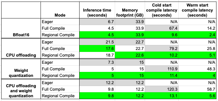
Looking closely at the table above, we can immediately see that regional compilation provides speed-ups almost similar to full compilation, while being significantly faster in terms of compilation time.
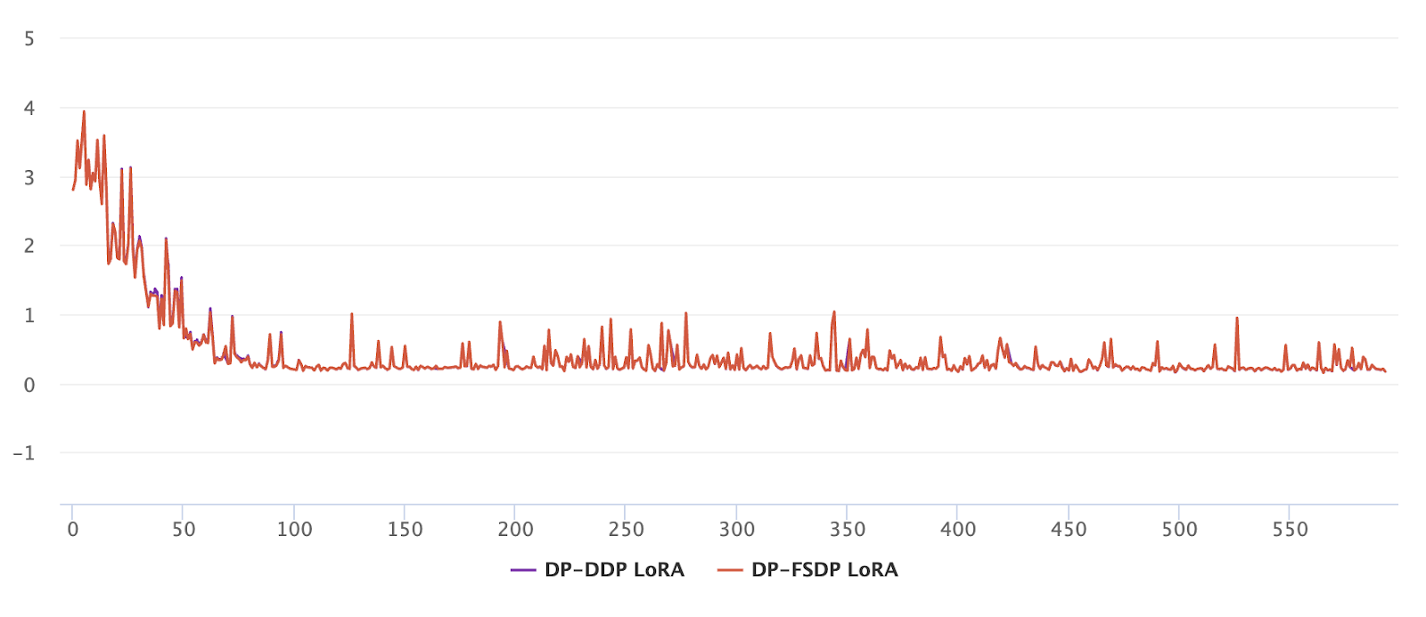
LoRA adapters

LoRA adapters let you personalize a base diffusion model without fine‑tuning millions of parameters. The downside is that switching between adapters normally swaps weight tensors inside the DiT, forcing torch.compile to re‑trace and re‑compile.

Diffusers now integrates PEFT’s LoRA hot‑swap to dodge that hit. You declare the maximum LoRA rank you’ll need, compile once, and then swap adapters on the fly. No recompilation required.

pipe = FluxPipeline.from_pretrained(

    "black-forest-labs/FLUX.1-dev", torch_dtype=torch.bfloat16

).to("cuda")

pipe.enable_lora_hotswap(target_rank=max_rank)

pipe.load_lora_weights(<lora-adapter-name1>)

pipe.transformer.compile(fullgraph=True)

# from this point on, load new LoRAs with `hotswap=True`

pipe.load_lora_weights(<lora-adapter-name2>, hotswap=True)

Because only the LoRA weight tensors change and their shapes stay fixed, the compiled kernels remain valid and inference latency stays flat.

Caveats

  • We need to provide the maximum rank among all LoRA adapters ahead of time. Thus, if we have one adapter with rank 16 and another with 32, we need to pass `max_rank=32`. 
  • LoRA adapters that are hotswapped can only target the same layers, or a subset of layers, that the first LoRA targets.
  • Hot‑swapping the text encoder is not yet supported.

For more details, see the LoRA hot‑swap docs and the test suite.

LoRA inference integrates seamlessly with the offloading and quantization features discussed above. If you’re constrained by GPU VRAM, please consider using them.

Operational Hardening

Diffusers runs a dedicated CI job nightly to keep torch.compile support robust. The suite exercises the most popular pipelines and automatically checks for:

  • Graph breaks and silent fallbacks
  • Unintended recompilations across common input shapes
  • Compatibility between compilation, CPU offloading, and every quantization backend we support

Interested readers are encouraged to check out this link to look at recent PRs that improve torch.compile coverage.
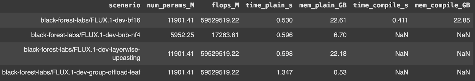
Benchmarks

Correctness is only half the story; we care about performance too. A revamped benchmarking workflow now runs alongside CI, capturing latency and peak memory for each scenario covered in this post. Results are exported to a consolidated CSV so regressions (or wins!) are easy to spot. The design and early numbers live in this PR.

Conclusion

torch.compile can turn a standard Diffusers pipeline into a high‑performance, memory‑efficient workhorse. By focusing compilation on the DiT, leveraging regional compilation and dynamic shapes, and stacking the compiler with offloading, quantization, and LoRA hot‑swap, you can unlock substantial speed‑ups and VRAM savings without sacrificing image quality or flexibility.

We hope these recipes inspire you to weave torch.compile into your own diffusion workflows. We’re excited to see what you build next.

Happy compiling ⚡

The Diffusers team would like to acknowledge the help and support of Animesh and Ryan in improving the torch.compile support.

Links to Important Resources

Read More

Enabling Fully Sharded Data Parallel (FSDP2) in Opacus

Introduction and Context

Opacus is making significant strides in supporting private training of large-scale models with its latest enhancements. Recently, we introduced Fast Gradient Clipping (FGC) and Ghost Clipping (GC), which enabled developers and researchers to perform gradient clipping without instantiating the per-sample gradients. These methods reduce the memory footprint of DP-SGD compared to the native Opacus implementation that relies on hooks.

Even with these advancements, training large-scale models such as Large Language Models (LLMs) remains a significant challenge for Opacus. As the demand for private training of large-scale models continues to grow, it is crucial for Opacus to support both data and model parallelism techniques. Currently, Opacus supports Differentially Private Distributed Data Parallel (DPDDP) to enable multi-GPU training. While DPDDP effectively scales model training across multiple GPUs and nodes, it requires each GPU to store a copy of the model and optimizer states, leading to high memory requirements, especially for large models.

This limitation underscores the need for alternative parallelization techniques, such as Fully Sharded Data Parallel (FSDP), which can offer improved memory efficiency and increased scalability via model, gradients, and optimizer states sharding. In the context of training Llama or other large language models, different parallelism strategies are typically employed to scale the training depending on the model size:

  • 1D Parallelism: DDP or FSDP for small-sized models (<10 billion parameters).
  • 2D Parallelism: FSDP combined with Tensor Parallelism (TP) for medium-sized models (10-100 billion parameters).
  • 4D Parallelism: FSDP combined with TP, Pipeline Parallelism (PP), and Context Parallelism (CP) for large-sized models (>100 billion parameters).

By adopting FSDP (example), Opacus is enhancing its capability to facilitate more efficient and scalable private training or fine-tuning of LLMs. This development marks a promising step forward in meeting the evolving needs of the ML community, paving the way for advanced parallelism strategies such as 2D and 4D parallelism to support private training of medium to large-scale models.

FSDP with FGC and GC

Fully Sharded Data Parallelism (FSDP) is a powerful data parallelism technique that enables the training of larger models by efficiently managing memory usage across multiple GPU workers. FSDP allows for the sharding of model parameters, gradients, and optimizer states across workers, which significantly reduces the memory footprint required for training. Although this approach incurs additional communication overhead due to parameter gathering and discarding during training, the cost is often mitigated by overlapping it with computation.

In FSDP, even though the computation for each microbatch of data is still local to each GPU worker, the full parameters are gathered for one block (e.g., a layer) at a time resulting in lower memory footprint. Once a block is processed, each GPU worker discards the parameter shards collected from other workers, retaining only its local shard. Consequently, the peak memory usage is determined by the maximum size of parameters+gradients+optimizer_states per layer, as well as the total size of activations, which depends on the per-device batch size. For more details on FSDP, please refer to the PyTorch FSDP paper.

The flow of FSDP with FGC or GC is as follows:

  • Forward pass
    • For each layer in layers:
      • [FSDP hook] all_gather full parameters of layer
      • Forward pass for layer
      • [FSDP hook] Discard full parameters of layer
      • [Opacus hook] Store the activations of layer
  • Reset optimizer.zero_grad()
  • First backward pass
    • For each layer in layers:
      • [FSDP hook] all_gather full parameters of layer
      • Backward pass for layer
      • [Opacus hook] compute per-sample gradient norms using FGC or GC
      • [FSDP hook] Discard full parameters of layer
      • [FSDP hook] reduce_scatter gradients of layer → not necessary
  • Rescale the loss function using the per-sample gradient norms
  • Reset oprimizer.zero_grad()
  • Second backward pass
    • For each layer in layers:
      • [FSDP hook] all_gather full parameters of layer
      • Backward pass for layer
      • [FSDP hook] Discard full parameters of layer
      • [FSDP hook] reduce_scatter gradients of layer
  • Add noise on each device to the corresponding shard of parameters
  • Apply optimizer step on each device to the corresponding shard of parameters

Figure 1: Workflow of FSDP based Fast Gradient Clipping or Ghost Clipping in Opacus. Note that there is an overlap between compute and communication – 1) In the forward pass: computation of the current layer (l) is overlapped with the all_gather of next layer’s (l+1) parameter. 2) In the backward pass: gradient computation of the current layer (l) is overlapped with the reduce_scatter of the previous layer’s (l+1) gradients and all_gather of the next layer’s (l-1) parameter.

How to use FSDP in Opacus

The training loop is identical to that of the standard PyTorch loop. As in Opacus before, we use

  • PrivacyEngine(), which configures the model and optimizer for running DP-SGD.
  • To enable Ghost Clipping with FSDP, the argumentgrad_sample_mode="ghost_fsdp" is used.
  • Additionally, we wrap the model with FSDP2Wrapperbefore initializing the optimizer and callingmake_private()

FSDP2Wrapper applies FSDP2 (second version of FSDP) to the root module and also to each torch.nn layer that does not require functorch to compute per-sample gradient norms. Layer types that depend on functorch are not separately wrapped with FSDP2 and thus fall into the root module’s communication group. The layers that are attached to the root module’s communication group will be unsharded first (at the beginning of forward/backward pass) and resharded the last (after the entire forward/backward pass). This will impact the peak memory as layers attached to the root module will not be resharded immediately after that layer is executed.

We use FSDP2 in our implementation as the previous version (FSDP) is not compatible with two backward passes setup of Ghost Clipping.

from opacus import PrivacyEngine
from opacus.utils.fsdp_utils import FSDP2Wrapper

def launch(rank, world_size):
   torch.cuda.set_device(rank)
   setup_distributed_env(rank, world_size)
   criterion = nn.CrossEntropyLoss() # example loss function
   model     = ToyModel()
   model     = FSDP2Wrapper(model) # different from DPDDP wrapper
   optimizer = optim.SGD(model.parameters(), lr=args.lr)

   privacy_engine = PrivacyEngine()
   model_gc, optimizer_gc, criterion_gc, train_loader, = privacy_engine.make_private(
           module=model,
           optimizer=optimizer,
           data_loader=train_loader,
           noise_multiplier=noise_multiplier
           max_grad_norm=max_grad_norm,
           criterion=criterion,
           grad_sample_mode="ghost_fsdp",)

   # The training loop below is identical to that of PyTorch
   for input_data, target_data in train_loader:
       input_data, target_data = input_data.to(rank), target_data.to(rank)
       output_gc = model_gc(input_data) # Forward pass
       optimizer_gc.zero_grad()
       loss = criterion_gc(output_gc, target_data)
       loss.backward()
       optimizer_gc.step()  # Add noise and update the model

world_size = torch.cuda.device_count()
mp.spawn(
       launch,
       args=(world_size,),
       nprocs=world_size,
       join=True,
   )

Memory Analysis

We provide results on memory consumption with full fine-tuning of GPT2 series of models. We only train the transformer blocks; the embedding layers (token embedding layer, positional embedding layer) are frozen.

Figure 2 reports the maximum batch size supported by FSDP2 vs DPDDP when training the model with the Ghost Clipping method. With FSDP2, we can achieve a 2.6x larger batch size for a 1.5B parameter GPT2 model on 1×8 A100 40GB GPUs, compared to using DPDDP. FSDP2 shows significant improvements for larger models (>1B) where the size of parameters and optimizer states dominates the activations.

Figure 2: Maximum batch size on a 1×8 A100 40GB GPU node while training a series of GPT2 models with Ghost Clipping based DP-SGD. We used the Shakespeare Dataset with a maximum sequence length of 1024 and float32 AdamW optimizer.

Table 1 presents the peak memory for a given step and total occupied memory after the execution of the step. Notably, the total memory of FSDP2 after model initialization is 8x lower than that of DPDDP since FSDP2 shards the model across 8 GPUs. The forward pass, for both FSDP2 and DPDDP, roughly increases the peak memory by ~10GB as activations are not sharded in both types of parallelism. For the backward pass and optimizer step, the peak memory for DPDDP is proportional to the model size whereas for FSDP2 it is proportional to the model size divided by the number of workers. Typically, as model sizes increase, the advantages of FSDP2 become even more pronounced.

Table 1: Memory estimates on rank 0 when training GPT2-xl model (1.5B) with Ghost Clipping based DP-SGD (AdamW optimizer, iso batch size of 16) on 1×8 A100 40GB GPU node. Peak Memory indicates the maximum memory allotted during the step, and total memory is the amount of occupied memory after executing the given step.

DPDDP  FSDP2
Peak Memory (GB) Total Memory (GB) Peak Memory (GB) Total Memory (GB)
Model initialization 5.93 5.93 1.08 0.78
Forward Pass 16.17 16.13 11.31 10.98
GC Backward Pass 22.40 11.83 12.45 1.88
Optimizer step 34.15 28.53 3.98 3.29
Optimizer zero grad 28.53 17.54 3.29 2.59

Latency Analysis

Table 2 shows the max batch size and latency numbers for LoRA fine-tuning of the Llama-3 8B model with DP-DDP and FSDP2. We observe that, for DP-SGD with Ghost Clipping, FSDP2 supports nearly twice the batch size but has lower throughput (0.6x) as compared to DP-DDP with hooks for the same effective batch size. In this particular setup, with LoRA fine-tuning, using FSDP2 does not result in any significant improvements. However, if the dataset has samples with a sequence length of 4096, which DP-DDP cannot accommodate, FSDP2 becomes necessary.

Table 2a: LoRA fine-tuning of Llama-3 8B with (trainable parameters: 6.8M) on Tiny Shakespeare dataset, AdamW optimizer with 32-bit precision, max sequence length of 512, 1×8 A100 80GB GPUs. Here, we do not use any gradient accumulation.

Training Method Parallelism Max batch size per device Total batch size Tokens per second Samples per second
SGD

(non-private)

DP-DDP 4 32 18,311 ± 20 35.76 ± 0.04
FSDP2 4 32 13,158 ± 498 25.70 ± 0.97
8 64 16,905 ± 317 33.02 ± 0.62
DP-SGD with Hooks DP-DDP 4 32 17,530 ± 166 34.24 ± 0.32
DP-SGD with Ghost Clipping DP-DDP 4 32 11,602 ± 222 22.66 ± 0.43
 

FSDP2

4 32 8,888 ± 127 17.36 ± 0.25
8 64 10,847 ± 187 21.19 ± 0.37

Table 2b: LoRA fine-tuning of Llama-3 8B with (trainable parameters: 6.8M) on Tiny Shakespeare dataset, AdamW optimizer with 32-bit precision, max sequence length of 512, 1×8 A100 80GB GPUs. Here, we enable gradient accumulation to increase the total batch size to 256. 

Training Method Parallelism Max batch size per device Gradient accumulation steps Total batch size Tokens per second Samples per second
DP-SGD with Hooks DP-DDP 4 8 256 17,850 ± 61 34.86 ± 0.12
DP-SGD with Ghost Clipping DP-DDP 4 8 256 12,043 ± 39 23.52 ± 0.08
FSDP2 8 4 256 10,979 ± 103 21.44 ± 0.20

Table 3 presents the throughput numbers for full fine-tuning of Llama-3 8B. Currently, FSDP2 with Ghost Clipping does not support tied parameters (embedding layers). We freeze these layers during fine-tuning, which brings the trainable parameters down from 8B to 7.5B. As shown in Table 3, DP-DDP throws an OOM error even with batch size 1 per device. Whereas, with FSDP2, each device can fit a batch size of 8 enabling full fine-tuning of Llama-3 8B.

To compare full fine-tuning of FSDP2 with DP-DDP, we shift from AdamW optimizer to SGD w/o momentum and reduce the trainable parameters from 7.5B to 5.1B by freezing normalization layers’ and gate projection layers’ weights. This allows DP-DDP to run with a batch size of 2 (1 if gradient accumulation is enabled). In this setting, we observe that FSDP2 is 1.65x times faster than DP-DDP for iso batch size.

Table 3: Ghost Clipping DP-SGD based full fine-tuning of Llama-3 8B on Tiny Shakespeare dataset, max sequence length of 512, 1×8 A100 80GB GPUs.

Setup Parallelism Max batch size per device Gradient accumulation steps Total batch size Tokens per second Samples per second
Trainable parameters: 7.5B
Optimizer: AdamW
DP-DDP 1 1 8 OOM OOM
FSDP2 8 1 64 6,442 ± 68 12.58 ± 0.13
Trainable parameters: 5.1B
Optimizer: SGD
DP-DDP 2 1 16 5,173 ± 266 10.10 ± 0.52
FSDP2 2 1 16 4,230 ± 150 8.26 ± 0.29
DP-DDP 2 4 64 OOM OOM
1 8 64 4,762 ± 221 9.30 ± 0.43
FSDP2 8 1 64 7,872 ± 59 15.37 ± 0.12

Correctness Verification

We did an integration test of Ghost Clipping DP-SGD with FSDP on an internal Meta use case, consisting of a Llama-3 8B model with LoRA fine-tuning for the next word prediction task. Our results show that Ghost Clipping with FSDP has roughly the same train loss (negligible difference) as DP-DDP. The previous results, as well as the unit test (link) have proved the correctness of the implementation.

Figure 3: Training loss (y-axis) vs iterations (x-axis) for LoRA fine-tuning of Llama-3 8B using Ghost Clipping DP-SGD for next word prediction task.

Limitations

The current version of FSDP does not support the following scenarios:

  1. Layers with tied parameters.
  2. Freezing/unfreezing the trainable parameters within the training phase.

The following are the two main limitations with the current implementation of gradient accumulation with FSDP2 Ghost Clipping.

    • Latency:
      • The current implementation of gradient accumulation with FSDP2 synchronizes the gradients after every backward pass. Since Ghost Clipping has two backward passes, we have 2k gradient synchronization calls (reduce_scatter) for k gradient accumulation steps.
      • This is because no_sync can’t be directly used when there are two backward passes for each forward pass.
      • Ideally, we should have only 1 gradient synchronization call for k gradient accumulation steps.
      • The latency of reduce_scatter is negligible in case of LoRA fine-tuning. Also, with a reasonable compute / communication overlap, this overhead can be masked.
  • Memory:
    • Gradient accumulation uses an additional buffer to store the accumulated gradients (sharded) irrespective of the number of gradient accumulation steps.
    • We would like to avoid the usage of an additional buffer when the number of gradient accumulation steps is equal to one. This is not specific to FSDP2 and is a bottleneck for the Opacus library in general.

Main takeaway

  • For models with small size of trainable parameters, e.g. LoRA fine-tuning
    • It is recommended to use DP-DDP with gradient accumulation whenever possible.
    • Shift to FSDP2 if DP-DDP throws an OOM error for the required sequence length or model size.
  • For full fine-tuning with a reasonably large number of trainable parameters
    • It is recommended to use FSDP2 as it has higher throughput than DP-DDP
    • In most cases, FSDP2 is the only option as DP-DDP triggers OOM even with a batch size of one.
  • The above observations hold for both private and non-private cases.

Conclusion

In this post, we present the integration of Fully Sharded Data Parallel (FSDP) with Fast Gradient Clipping (FGC) and Ghost Clipping (GC) in Opacus, demonstrating its potential to scale the private training of large-scale models with over 1 billion trainable parameters. By leveraging FSDP, we have shown that it is possible to fully fine-tune the Llama-3 8B model, a feat that is not achievable with Differentially Private Distributed Data Parallel (DP-DDP) due to memory constraints.

The introduction of FSDP in Opacus marks a significant advancement to the Opacus library, offering a scalable and memory-efficient solution for private training of LLMs. This development not only enhances the capability of Opacus to handle large-scale models but also sets the stage for future integration of other model parallelism strategies.

Looking ahead, our focus will be on enabling 2D parallelism with Ghost Clipping and integrating FSDP with native Opacus using hooks. These efforts aim to further optimize the training process, reduce latency, and expand the applicability of Opacus to even larger and more complex models. We are excited about the possibilities that these advancements will unlock and are committed to pushing the boundaries of what is possible in private machine learning. Furthermore, we invite developers, researchers, and enthusiasts to join us in this journey. Your contributions and insights are invaluable as we continue to enhance Opacus.

Acknowledgments

We would like to thank Will Bullock, Wei Feng, Ilya Mironov, and Iden Kalemaj for their technical review and guidance.

Read More

Reducing Storage Footprint and Bandwidth Usage for Distributed Checkpoints with PyTorch DCP

Summary

PyTorch Distributed Checkpointing (DCP) is a versatile and powerful tool for managing model checkpoints in distributed training environments. Its modular design empowers developers to tailor its components to their specific requirements, making it an ideal solution for a wide range of use cases.

In this blog post, we’ll showcase how we leveraged PyTorch DCP’s modularity to integrate compression and achieve a 22% reduction in checkpoint size. We’ll also provide a deep dive into the implementation details of our customization, offering practical insights and guidance on how you can apply similar techniques to optimize your own checkpointing workflows and improve overall efficiency.

Motivation

Large Distributed Checkpoints

As models increase in complexity and size, distributed checkpointing becomes a critical component of the training process. However, these checkpoints often result in substantial storage demands and elevated bandwidth costs due to their large sizes.

Compression

To address this challenge, compression emerges as a natural solution. Given that checkpoints primarily consist of binary data (tensors), we aimed for an optimal compression ratio with minimal compression overhead. We chose the zstd compression algorithm for its efficiency and effectiveness.

DCP

The modular design of DCP, featuring well-defined and easily extensible components, made it an ideal choice as our checkpointing solution.

Details

Customizing StorageWriter

PyTorch DCP’s StorageWriter component is responsible for writing checkpoint data to storage. We customized this component by modifying _FileSystemWriter, which extends the base StorageWriter class. The _FileSystemWriter class now takes an additional parameter _extension, which is an instance of StreamTransformExtension.

def save(
    state_dict: STATE_DICT_TYPE,
    *,
    checkpoint_id: Union[str, os.PathLike, None] = None,
    # We used a _FileSystemWriterextended as a storage writer component
    storage_writer: Optional[StorageWriter] = None, 
    planner: Optional[SavePlanner] = None,
    process_group: Optional[dist.ProcessGroup] = None,
    no_dist: bool = False,
) -> Metadata:

class _FileSystemWriter(StorageWriter):

    def __init__(
        self,
        path: Union[str, os.PathLike],
        single_file_per_rank: bool = True,
        sync_files: bool = True,
        thread_count: int = 1,
        per_thread_copy_ahead: int = 10_000_000,
        overwrite: bool = True,
 # We customized _FileSystemWriterextended to take in an extension
        _extensions: Optional[Sequence[StreamTransformExtension]] = None,
        serialization_format: SerializationFormat = SerializationFormat.TORCH_SAVE,
        *args: Any,
        **kwargs: Any,
    ) -> None:

StreamTransformExtension is an abstract class that defines two methods: transform_to(), which is called on an output stream, and transform_from(), which is called on an input stream. These enable us to perform custom transformations on the stream data.

class StreamTransformExtension(Extension):

    @abc.abstractmethod
    def transform_to(self, output: IO[bytes]) -> IO[bytes]:

    @abc.abstractmethod
    def transform_from(self, input: IO[bytes]) -> IO[bytes]:

Implementing ZStandard Compression

We implemented a concrete subclass of StreamTransformExtension called ZStandard, which provides compression functionality using the zstd compression algorithm. Our ZStandard class implements the transform_to() to compress the outgoing stream data and the transform_from() to decompress the incoming stream data.

class ZStandard(StreamTransformExtension):

    def transform_to(self, output: IO[bytes]) -> IO[bytes]:
# Our compression implementation

    def transform_from(self, input: IO[bytes]) -> IO[bytes]:
# Our decompression implementation

Combining Customizations

Finally, we combined our custom _FileSystemWriter class with the ZStandard compression extension while saving the checkpoint. We wrote a sample test to demonstrate how everything comes together

fs_writer = FileSystemWriter(
          path=path,
          thread_count=thread_count,
         _extensions=[ZStandard()],
)

save(
         state_dict=state_dict_to_save,
         storage_writer=fs_writer,
)

Evaluation

Results

In collaboration with IBM, we conducted an evaluation of our proposed solution on one of their internal training clusters. The results showed a significant 22% reduction in checkpoint sizes, albeit at the cost of increased compression time. However, with multi-threading, we were able to mitigate this trade-off and limit the increase in checkpointing time to just 9%. This demonstrates the potential of our solution to strike a balance between checkpoint size reduction and performance.

Model Threads per Rank DCP Checkpoint Size (in GB) Checkpointing Time (s)
Baseline ZStd 𝚫 Baseline ZStd 𝚫
granite-3b-code-instruct 8 6.72 5.26 -21.8% 1.96 2.15 9.7%
4 6.72 5.26 -21.8% 1.98 2.38 20.2%
1 6.72 5.26 -21.8% 2.34 3.86 64.9%
granite-3.2-8b-instruct 8 15.6 12.08 –22.5% 3.37 3.65 8.3%
4 15.6 12.08 –22.5% 3.72 4.37 17.5%
1 15.6 12.08 –22.5% 5.37 8.45 57.4%

Setup

We chose two of IBM’s open sourced models (Granite-3B-Code-Instruct-128K and Granite-3.2-8B-Instruct). For evaluation, we perform full-parameter FSDP fine-tuning on these models with the Alpaca dataset on IBM’s Vela AI supercomputer, which is housed in IBM cloud. Each of Vela’s nodes has eight 80GB A100 GPUs, which are connected to each other by NVLink and NVSwitch. In addition, each node has two 2nd Generation Intel Xeon Scalable processors (Cascade Lake) and 1.5TB of DRAM. We provision one node of Vela with the following resources:

Testbed

  • Openshift 4.14 Cluster
  • Pod: 64 Intel Cascade Lake CPU cores, 800GB host memory, 8 x A100-80GB GPUs
  • Storage options exposed as persistent volumes:
    • 1TB local GPFS
    • S3 bucket

Workload

  • Full-parameter FSDP finetuning with checkpointing every epoch

Checkpointing configuration

  • save_state_dict() to storage
  • 1 to 8 threads per rank
  • 1 file per rank
  • 8 ranks

Conclusion

PyTorch DCP’s modular design empowers developers to tailor its components to specific use cases, unlocking new levels of customization and extensibility. By customizing the StorageWriter component and implementing a compression extension, we achieved significant checkpoint size reductions, leading to lower storage requirements, and reduced bandwidth costs.

We invite you to explore the vast possibilities of PyTorch DCP customization by diving into our documentation and experimenting with various extensions and modifications. Join the conversation on PyTorch GitHub and connect with the PyTorch Checkpointing team (open GitHub issue with label “oncall: distributed checkpointing”) to share your experiences, ask questions, and stay up-to-date on the latest developments!

Read More