3 Questions: John Leonard on the future of autonomous vehicles

As part of the MIT Task Force on the Work of the Future’s new series of research briefs, Professor John Leonard teamed with professor of aeronautics and astronautics and of history David Mindell and with doctoral candidate Erik Stayton to explore the future of autonomous vehicles (AV) — an area that could arguably be called the touchstone for the discussion of jobs of the future in recent years. Leonard is the Samuel C. Collins Professor of Mechanical and Ocean Engineering in the Department of Mechanical Engineering, a member of the Computer Science and Artificial Intelligence Laboratory (CSAIL), and member of the MIT Task Force on the Work of the Future. His research addresses navigation and mapping for autonomous mobile robots operating in challenging environments. 

Their research brief, Autonomous Vehicles, Mobility, and Employment Policy: The Roads Ahead,” looks at how the AV transition will affect jobs and explores how sustained investments in workforce training for advanced mobility can help drivers and other mobility workers transition into new careers that support mobility systems and technologies. It also highlights the policies that will greatly ease the integration of automated systems into urban mobility systems, including investing in local and national infrastructure, and forming public-private partnerships. Leonard spoke recently on some of the findings in the brief.

Q: When would you say Level 4 autonomous vehicle systems — those that can operate without active supervision by a human driver — increase their area of operation beyond today’s limited local deployments?

A: The widespread deployment of Level 4 automated vehicles will take much longer than many have predicted — at least a decade for favorable environments, and possibly much longer. Despite substantial recent progress by the community, major challenges remain before we will see the disruptive rollout of fully automated driving systems that have no safety driver onboard over large areas. Expansion will likely be gradual, and will happen region-by-region in specific categories of transportation, resulting in wide variations in availability across the country. The key question is not just “when,” but “where” will the technology be available and profitable?

Driver assistance and active safety systems (known as Level 2 automation) will continue to become more widespread on personal vehicles. These systems, however, will have limited impacts on jobs, since a human driver must be on board and ready to intervene at any moment. Level 3 systems can operate without active engagement by the driver for certain geographic settings, so long as the driver is ready to intervene when requested; however, these systems will likely be restricted to low-speed traffic.

Impacts on trucking are also expected to be less than many have predicted, due to technological challenges and risks that remain, even for more structured highway environments.

Q: In the brief, you make the argument that AV transition, while threatening numerous jobs, will not be “jobless.” Can you explain?  What are the likely impacts to mobility jobs — including transit, vehicle sales, vehicle maintenance, delivery, and other related industries?

A: The longer rollout time for Level 4 autonomy provides time for sustained investments in workforce training that can help drivers and other mobility workers transition into new careers that support mobility systems and technologies. Transitioning from current-day driving jobs to these jobs represents potential pathways for employment, so long as job-training resources are available. Because the geographical rollout of Level 4 automated driving is expected to be slow, human workers will remain essential to the operation of these systems for the foreseeable future, in roles that are both old and new. 

In some cases, Level 4 remote driving systems could move driving jobs from vehicles to fixed-location centers, but these might represent a step down in job quality for many professional drivers. The skills required for these jobs is largely unknown, but they are likely to be a combination of call-center, dispatcher, technician, and maintenance roles with strong language skills. More advanced engineering roles could also be sources of good jobs if automated taxi fleets are deployed at scale, but will require strong technical training that may be out of reach for many. 

Increasing availability of Level 2 and Level 3 systems will result in changes in the nature of work for professional drivers, but do not necessarily impact job numbers to the extent that other systems might, because these systems do not remove drivers from vehicles. 

While the employment implications of widespread Level 4 automation in trucking could eventually be considerable, as with other domains, the rollout is expected to be gradual. Truck drivers do more than just drive, and so human presence within even highly automated trucks would remain valuable for other reasons such as loading, unloading, and maintenance. Human-autonomous truck platooning, in which multiple Level 4 trucks follow a human-driven lead truck, may be more viable than completely operator-free Level 4 operations in the near term.  

Q: How should we prepare policy in the three key areas of infrastructure, jobs, and innovation? 

A: Policymakers can act now to prepare for and minimize disruptions to the millions of jobs in ground transportation and related industries that may come in the future, while also fostering greater economic opportunity and mitigating environmental impacts by building safe and accessible mobility systems. Investing in local and national infrastructure, and forming public-private partnerships, will greatly ease integration of automated systems into urban mobility systems.  

Automated vehicles should be thought of as one element in a mobility mix, and as a potential feeder for public transit rather than a replacement for it, but unintended consequences such as increased congestion remain risks. The crucial role of public transit for connecting workers to workplaces will endure: the future of work depends in large part on how people get to work.

Policy recommendations in the trucking sector include strengthening career pathways for drivers, increasing labor standards and worker protections, advancing public safety, creating good jobs via human-led truck platooning, and promoting safe and electric trucks.

Read More

AI Explains AI: Fiddler Develops Model Explainability for Transparency

Your online loan application just got declined without explanation. Welcome to the AI black box.

Businesses of all stripes turn to AI for computerized decisions driven by data. Yet consumers using applications with AI get left in the dark on how automated decisions work. And many people working within companies have no idea how to explain the inner workings of AI to customers.

Fiddler Labs wants to change that.

The San Francisco-based startup offers an explainable AI platform that enables companies to explain, monitor and analyze their AI products.

Explainable AI is a growing area of interest for enterprises because those outside of engineering often need to understand how their AI models work.

Using explainable AI, banks can provide reasons to customers for a loan’s rejection, based on data points fed to models, such as maxed credit cards or high debt-to-income ratios. Internally, marketers can strategize about customers and products by knowing more about the data points that drive them.

“This is bridging the gap between hardcore data scientists who are building the models and the business teams using these models to make decisions,” said Anusha Sethuraman, head of product marketing at Fiddler Labs.

Fiddler Labs is a member of NVIDIA Inception, a program that enables companies working in AI and data science with fundamental tools, expertise and marketing support, and helps them get to market faster.

What Is Explainable AI?

Explainable AI is a set of tools and techniques that help explore the math inside an AI model. It can map out the data inputs and their weighted values that were used to arrive at the data output of the model.

All of this, essentially, enables a layperson to study the sausage factory at work on the inside of an otherwise opaque process. The result is explainable AI can help deliver insights into how and why a particular decision was made by a model.

“There’s often a hurdle to get AI into production. Explainability is one of the things that we think can address this hurdle,” Sethuraman said.

With an ensemble of models often at use, creating this is no easy job.

But Fiddler Labs CEO and co-founder Krishna Gade is up to the task. He previously led the team at Facebook that built the “Why am I seeing this post?” feature to help consumers and internal teams understand how its AI works in the Facebook news feed.

He and Amit Paka — a University of Minnesota classmate — joined forces and quit their jobs to start Fiddler Labs. Paka, the company’s chief product officer, was motivated by his experience at Samsung with shopping recommendation apps and the lack of understanding into how these AI recommendation models work.

Explainability for Transparency

Founded in 2018, Fiddler Labs offers explainability for greater transparency in businesses. It helps companies make better informed business decisions through a combination of data, explainable AI and human oversight, according to Sethuraman.

Fiddler’s tech is used by Hired, a talent and job matchmaking site driven by AI. Fiddler provides real-time reporting on how Hired’s AI models are working. It can generate explanations on candidate assessments and provide bias monitoring feedback, allowing Hired to assess its AI.

Explainable AI needs to be quickly available for consumer fintech applications. That enables customer service representatives to explain automated financial decisions — like loan rejections and robo rates — and build trust with transparency about the process.

The algorithms used for explanations require hefty processing. Sethuraman said that Fiddler Labs taps into NVIDIA cloud GPUs to make this possible, saying CPUs aren’t up to the task.

“You can’t wait 30 seconds for the explanations — you want explanations within milliseconds on a lot of different things depending on the use cases,” Sethuraman said.

Visit NVIDIA’s financial services industry page to learn more.

Image credit: Emily Morter, via the Unsplash Photo Community. 

The post AI Explains AI: Fiddler Develops Model Explainability for Transparency appeared first on The Official NVIDIA Blog.

Read More

Keeping a Watchful AI: NASA Project Aims to Predict Space Weather Events

While a thunderstorm could knock out your neighborhood’s power for a few hours, a solar storm could knock out electricity grids across all of Earth, possibly taking weeks to recover from.

To try to predict solar storms — which are disturbances on the sun — and their potential effects on Earth, NASA’s Frontier Development Lab (FDL) is running what it calls a geoeffectiveness challenge.

It uses datasets of tracked changes in the magnetosphere — where the Earth’s magnetic field interacts with solar wind — to train AI-powered models that can detect patterns of space weather events and predict their Earth-related impacts.

The training of the models is optimized on NVIDIA GPUs available on Google Cloud, and data exploration is done on RAPIDS, NVIDIA’s open-source suite of software libraries built to execute data science and analytics pipelines entirely on GPUs.

Siddha Ganju, a solutions architect at NVIDIA who was named to Forbes’ 30 under 30 list in 2018, is advising NASA on the AI-related aspects of the challenge.

A deep learning expert, Ganju grew up going to hackathons. She says she’s always been fascinated by how an algorithm can read in between the lines of code.

Now, she’s applying her knowledge to NVIDIA’s automotive and healthcare businesses, as well NASA’s AI technical steering committee. She’s also written a book on practical uses of deep learning, published last October.

Modeling Space Weather Impacts with AI

Ganju’s work with the FDL began in 2017, when its founder, James Parr, asked her to start advising the organization. Her current task, advising the geoeffectiveness challenge, seeks to use machine learning to characterize magnetic field perturbations and model the impact of space weather events.

In addition to solar storms, space weather events can include such activities as solar flares, which are sudden flashes of increased brightness on the sun, and solar wind, a stream of charged particles released from it.

Not all space weather events impact the Earth, said Ganju, but in case one does, we need to be prepared. For example, a single powerful solar storm could knock out our planet’s telephone networks.

“Even if we’re able to predict the impact of an event just 15 minutes in advance, that gives us enough time to sound the alarm and prepare for potential connectivity loss,” said Ganju. “This data can also be useful for satellites to communicate in a better way.”

Exploring Spatial and Temporal Patterns

Solar events can impact parts of the Earth differently due to a variety of factors, Ganju said. With the help of machine learning, the FDL is trying to find spatial and temporal patterns of the effects.

“The datasets we’re working with are huge, since magnetometers collect data on the changes of a magnetic field at a particular location every second,” said Ganju. “Parallel processing using RAPIDS really accelerates our exploration.”

In addition to Ganju, researchers Asti Bhatt, Mark Cheung and Ryan McGranaghan, as well as NASA’s Lika Guhathakurta, are advising the geoeffectiveness challenge team. Its members include Téo Bloch, Banafsheh Ferdousi, Panos Tigas and Vishal Upendran.

The researchers use RAPIDS to explore the data quickly. Then, using the PyTorch and TensorFlow software libraries, they train the models for experiments to identify how the latitude of a location, the atmosphere above it, or the way sun rays hit it affect the consequences of a space weather event.

They’re also studying whether an earthly impact happens immediately as the space event occurs, or if it has a delayed effect, as an impact could depend on time-related factors, such as the Earth’s revolutions around the sun or its rotation about its own axis.

To detect such patterns, the team will continue to train the model and analyze data throughout the duration of FDL’s eight-week research sprint, which concludes later this month.

Other FDL projects participating in the sprint, according to Ganju, include the moon for good challenge, which aims to discover the best landing position on the moon. Another is the astronaut health challenge, which is investigating how high-radiation environments can affect an astronaut’s well-being.

The FDL is holding a virtual U.S. Space Science & AI showcase, on August 14, where the 2020 challenges will be presented. Register for the event here.

Feature image courtesy of NASA.

The post Keeping a Watchful AI: NASA Project Aims to Predict Space Weather Events appeared first on The Official NVIDIA Blog.

Read More

Improving speech-to-text transcripts from Amazon Transcribe using custom vocabularies and Amazon Augmented AI

Businesses and organizations are increasingly using video and audio content for a variety of functions, such as advertising, customer service, media post-production, employee training, and education. As the volume of multimedia content generated by these activities proliferates, businesses are demanding high-quality transcripts of video and audio to organize files, enable text queries, and improve accessibility to audiences who are deaf or hard of hearing (466 million with disabling hearing loss worldwide) or language learners (1.5 billion English language learners worldwide).

Traditional speech-to-text transcription methods typically involve manual, time-consuming, and expensive human labor. Powered by machine learning (ML), Amazon Transcribe is a speech-to-text service that delivers high-quality, low-cost, and timely transcripts for business use cases and developer applications. In the case of transcribing domain-specific terminologies in fields such as legal, financial, construction, higher education, or engineering, the custom vocabularies feature can improve transcription quality. To use this feature, you create a list of domain-specific terms and reference that vocabulary file when running transcription jobs.

This post shows you how to use Amazon Augmented AI (Amazon A2I) to help generate this list of domain-specific terms by sending low-confidence predictions from Amazon Transcribe to humans for review. We measure the word error rate (WER) of transcriptions and number of correctly-transcribed terms to demonstrate how to use custom vocabularies to improve transcription of domain-specific terms in Amazon Transcribe.

To complete this use case, use the notebook A2I-Video-Transcription-with-Amazon-Transcribe.ipynb on the Amazon A2I Sample Jupyter Notebook GitHub repo.


Example of mis-transcribed annotation of the technical term, "an EC2 instance". This term was transcribed as “Annecy two instance”.

Example of mis-transcribed annotation of the technical term, “an EC2 instance”. This term was transcribed as “Annecy two instance”.


Example of correctly transcribed annotation of the technical term "an EC2 instance" after using Amazon A2I to build an Amazon Transcribe Custom Vocabulary and re-transcribing the video.

Example of correctly transcribed annotation of the technical term “an EC2 instance” after using Amazon A2I to build an Amazon Transcribe custom vocabulary and re-transcribing the video.


This walkthrough focuses on transcribing video content. You can modify the code provided to use audio files (such as MP3 files) by doing the following:

  • Upload audio files to your Amazon Simple Storage Service (Amazon S3) bucket and using them in place of the video files provided.
  • Modify the button text and instructions in the worker task template provided in this walkthrough and tell workers to listen to and transcribe audio clips.

Solution overview

The following diagram presents the solution architecture.


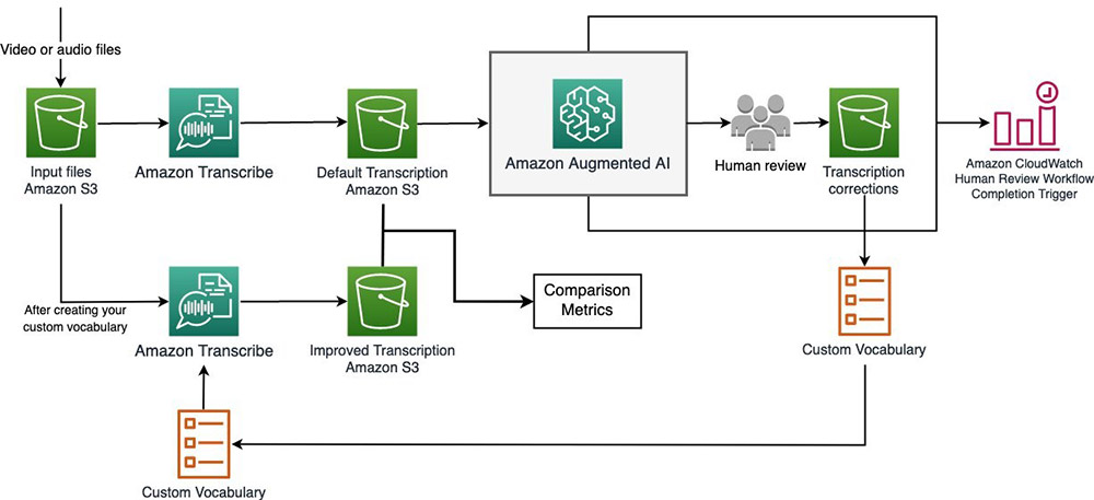
We briefly outline the steps of the workflow as follows:

  1. Perform initial transcription. You transcribe a video about Amazon SageMaker, which contains multiple mentions of technical ML and AWS terms. When using Amazon Transcribe out of the box, you may find that some of these technical mentions are mis-transcribed. You generate a distribution of confidence scores to see the number of terms that Amazon Transcribe has difficulty transcribing.
  2. Create human review workflows with Amazon A2I. After you identify words with low-confidence scores, you can send them to a human to review and transcribe using Amazon A2I. You can make yourself a worker on your own private Amazon A2I work team and send the human review task to yourself so you can preview the worker UI and tools used to review video clips.
  3. Build custom vocabularies using A2I results. You can parse the human-transcribed results collected from Amazon A2I to extract domain-specific terms and use these terms to create a custom vocabulary table.
  4. Improve transcription using custom vocabulary. After you generate a custom vocabulary, you can call Amazon Transcribe again to get improved transcription results. You evaluate and compare the before and after performances using an industry standard called word error rate (WER).

Prerequisites

Before beginning, you need the following:

  • An AWS account.
  • An S3 bucket. Provide its name in BUCKET in the notebook. The bucket must be in the same Region as this Amazon SageMaker notebook instance.
  • An AWS Identity and Access Management (IAM) execution role with required permissions. The notebook automatically uses the role you used to create your notebook instance (see the next item in this list). Add the following permissions to this IAM role:
    • Attach managed policies AmazonAugmentedAIFullAccess and AmazonTranscribeFullAccess.
    • When you create your role, you specify Amazon S3 permissions. You can either allow that role to access all your resources in Amazon S3, or you can specify particular buckets. Make sure that your IAM role has access to the S3 bucket that you plan to use in this use case. This bucket must be in the same Region as your notebook instance.
  • An active Amazon SageMaker notebook instance. For more information, see Create a Notebook Instance. Open your notebook instance and upload the notebook A2I-Video-Transcription-with-Amazon-Transcribe.ipynb.
  • A private work team. A work team is a group of people that you select to review your documents. You can choose to create a work team from a workforce, which is made up of workers engaged through Amazon Mechanical Turk, vendor-managed workers, or your own private workers that you invite to work on your tasks. Whichever workforce type you choose, Amazon A2I takes care of sending tasks to workers. For this post, you create a work team using a private workforce and add yourself to the team to preview the Amazon A2I workflow. For instructions, see Create a Private Workforce. Record the ARN of this work team—you need it in the accompanying Jupyter notebook.

To understand this use case, the following are also recommended:

Getting started

After you complete the prerequisites, you’re ready to deploy this solution entirely on an Amazon SageMaker Jupyter notebook instance. Follow along in the notebook for the complete code.

To start, follow the Setup code cells to set up AWS resources and dependencies and upload the provided sample MP4 video files to your S3 bucket. For this use case, we analyze videos from the official AWS playlist on introductory Amazon SageMaker videos, also available on YouTube. The notebook walks through transcribing and viewing Amazon A2I tasks for a video about Amazon SageMaker Jupyter Notebook instances. In Steps 3 and 4, we analyze results for a larger dataset of four videos. The following table outlines the videos that are used in the notebook, and how they are used.

Video # Video Title File Name Function

1

Fully-Managed Notebook Instances with Amazon SageMaker – a Deep Dive Fully-Managed Notebook Instances with Amazon SageMaker – a Deep Dive.mp4 Perform the initial transcription
and viewing sample Amazon A2I jobs in Steps 1 and 2.Build a custom vocabulary in Step 3

2

Built-in Machine Learning Algorithms with Amazon SageMaker – a Deep Dive Built-in Machine Learning Algorithms with Amazon SageMaker – a Deep Dive.mp4 Test transcription with the custom vocabulary in Step 4

3

Bring Your Own Custom ML Models with Amazon SageMaker Bring Your Own Custom ML Models with Amazon SageMaker.mp4 Build a custom vocabulary in Step 3

4

Train Your ML Models Accurately with Amazon SageMaker Train Your ML Models Accurately with Amazon SageMaker.mp4 Test transcription with the custom vocabulary in Step 4

In Step 4, we refer to videos 1 and 3 as the in-sample videos, meaning the videos used to build the custom vocabulary. Videos 2 and 4 are the out-sample videos, meaning videos that our workflow hasn’t seen before and are used to test how well our methodology can generalize to (identify technical terms from) new videos.

Feel free to experiment with additional videos downloaded by the notebook, or your own content.

Step 1: Performing the initial transcription

Our first step is to look at the performance of Amazon Transcribe without custom vocabulary or other modifications and establish a baseline of accuracy metrics.

Use the transcribe function to start a transcription job. You use vocab_name parameter later to specify custom vocabularies, and it’s currently defaulted to None. See the following code:

transcribe(job_names[0], folder_path+all_videos[0], BUCKET)

Wait until the transcription job displays COMPLETED. A transcription job for a 10–15-minute video typically takes up to 5 minutes.

When the transcription job is complete, the results is stored in an output JSON file called YOUR_JOB_NAME.json in your specified BUCKET. Use the get_transcript_text_and_timestamps function to parse this output and return several useful data structures. After calling this, all_sentences_and_times has, for each transcribed video, a list of objects containing sentences with their start time, end time, and confidence score. To save those to a text file for use later, enter the following code:

file0 = open("originaltranscript.txt","w")
    for tup in sentences_and_times_1:
        file0.write(tup['sentence'] + "n")
file0.close()

To look at the distribution of confidence scores, enter the following code:

from matplotlib import pyplot as plt
plt.style.use('ggplot')

flat_scores_list = all_scores[0]

plt.xlim([min(flat_scores_list)-0.1, max(flat_scores_list)+0.1])
plt.hist(flat_scores_list, bins=20, alpha=0.5)
plt.title('Plot of confidence scores')
plt.xlabel('Confidence score')
plt.ylabel('Frequency')

plt.show()

The following graph illustrates the distribution of confidence scores.

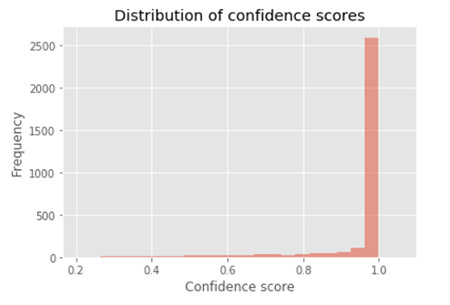
Next, we filter out the high confidence scores to take a closer look at the lower ones.

You can experiment with different thresholds to see how many words fall below that threshold. For this use case, we use a threshold of 0.4, which corresponds to 16 words below this threshold. Sequences of words with a term under this threshold are sent to human review.

As you experiment with different thresholds and observe the number of tasks it creates in the Amazon A2I workflow, you can see a tradeoff between the number of mis-transcriptions you want to catch and the amount of time and resources you’re willing to devote to corrections. In other words, using a higher threshold captures a greater percentage of mis-transcriptions, but it also increases the number of false positives—low-confidence transcriptions that don’t actually contain any important technical term mis-transcriptions. The good news is that you can use this workflow to quickly experiment with as many different threshold values as you’d like before sending it to your workforce for human review. See the following code:

THRESHOLD = 0.4

# Filter scores that are less than THRESHOLD
all_bad_scores = [i for i in flat_scores_list if i < THRESHOLD]
print(f"There are {len(all_bad_scores)} words that have confidence score less than {THRESHOLD}")

plt.xlim([min(all_bad_scores)-0.1, max(all_bad_scores)+0.1])
plt.hist(all_bad_scores, bins=20, alpha=0.5)
plt.title(f'Plot of confidence scores less than {THRESHOLD}')
plt.xlabel('Confidence score')
plt.ylabel('Frequency')

plt.show()

You get the following output:

There are 16 words that have confidence score less than 0.4

The following graph shows the distribution of confidence scores less than 0.4.

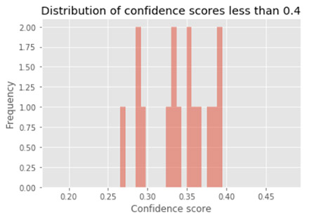
As you experiment with different thresholds, you can see a number of words classified with low confidence. As we see later, terms that are specific to highly technical domains are more difficult to automatically transcribe in general, so it’s important that we capture these terms and incorporate them into our custom vocabulary.

Step 2: Creating human review workflows with Amazon A2I

Our next step is to create a human review workflow (or flow definition) that sends low confidence scores to human reviewers and retrieves the corrected transcription they provide. The accompanying Jupyter notebook contains instructions for the following steps:

  1. Create a workforce of human workers to review predictions. For this use case, creating a private workforce enables you to send Amazon A2I human review tasks to yourself so you can preview the worker UI.
  2. Create a work task template that is displayed to workers for every task. The template is rendered with input data you provide, instructions to workers, and interactive tools to help workers complete your tasks.
  3. Create a human review workflow, also called a flow definition. You use the flow definition to configure details about your human workforce and the human tasks they are assigned.
  4. Create a human loop to start the human review workflow, sending data for human review as needed. In this example, you use a custom task type and start human loop tasks using the Amazon A2I Runtime API. Each time StartHumanLoop is called, a task is sent to human reviewers.

In the notebook, you create a human review workflow using the AWS Python SDK (Boto3) function create_flow_definition. You can also create human review workflows on the Amazon SageMaker console.

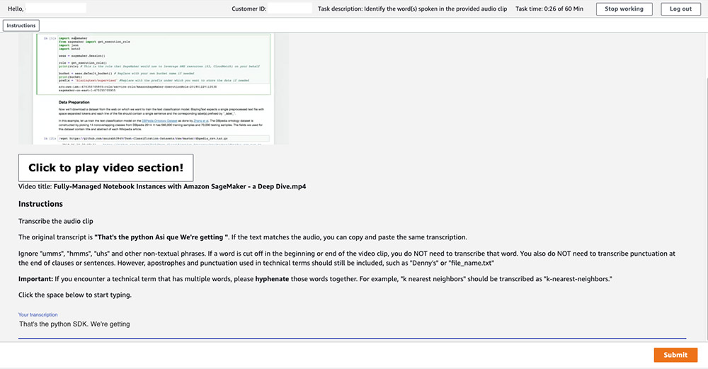
Setting up the worker task UI

Amazon A2I uses Liquid, an open-source template language that you can use to insert data dynamically into HTML files.

In this use case, we want each task to enable a human reviewer to watch a section of the video where low confidence words appear and transcribe the speech they hear. The HTML template consists of three main parts:

  • A video player with a replay button that only allows the reviewer to play the specific subsection
  • A form for the reviewer to type and submit what they hear
  • Logic written in JavaScript to give the replay button its intended functionality

The following code is the template you use:

<head>
    <style>
        h1 {
            color: black;
            font-family: verdana;
            font-size: 150%;
        }
    </style>
</head>
<script src="https://assets.crowd.aws/crowd-html-elements.js"></script>

<crowd-form>
    <video id="this_vid">
        <source src="{{ task.input.filePath | grant_read_access }}"
            type="audio/mp4">
        Your browser does not support the audio element.
    </video>
    <br />
    <br />
    <crowd-button onclick="onClick(); return false;"><h1> Click to play video section!</h1></crowd-button> 

    <h3>Instructions</h3>
    <p>Transcribe the audio clip </p>
    <p>Ignore "umms", "hmms", "uhs" and other non-textual phrases. </p>
    <p>The original transcript is <strong>"{{ task.input.original_words }}"</strong>. If the text matches the audio, you can copy and paste the same transcription.</p>
    <p>Ignore "umms", "hmms", "uhs" and other non-textual phrases.
    If a word is cut off in the beginning or end of the video clip, you do NOT need to transcribe that word.
    You also do NOT need to transcribe punctuation at the end of clauses or sentences.
    However, apostrophes and punctuation used in technical terms should still be included, such as "Denny's" or "file_name.txt"</p>
    <p><strong>Important:</strong> If you encounter a technical term that has multiple words,
    please <strong>hyphenate</strong> those words together. For example, "k nearest neighbors" should be transcribed as "k-nearest-neighbors."</p>
    <p>Click the space below to start typing.</p>
    <full-instructions header="Transcription Instructions">
        <h2>Instructions</h2>
        <p>Click the play button and listen carefully to the audio clip. Type what you hear in the box
            below. Replay the clip by clicking the button again, as many times as needed.</p>
    </full-instructions>

</crowd-form>

<script>
    var video = document.getElementById('this_vid');
    video.onloadedmetadata = function() {
        video.currentTime = {{ task.input.start_time }};
    };
    function onClick() {
        video.pause();
        video.currentTime = {{ task.input.start_time }};
        video.play();
        video.ontimeupdate = function () {
            if (video.currentTime >= {{ task.input.end_time }}) {
                video.pause()
            }
        }
    }
</script>

The {{ task.input.filePath | grant_read_access }} field allows you to grant access to and display a video to workers using a path to the video’s location in an S3 bucket. To prevent the reviewer from navigating to irrelevant sections of the video, the controls parameter is omitted from the video tag and a single replay button is included to control which section can be replayed.

Under the video player, the <crowd-text-area> HTML tag creates a submission form that your reviewer uses to type and submit.

At the end of the HTML snippet, the section enclosed by the <script> tag contains the JavaScript logic for the replay button. The {{ task.input.start_time }} and {{ task.input.end_time }} fields allow you to inject the start and end times of the video subsection you want transcribed for the current task.

You create a worker task template using the AWS Python SDK (Boto3) function create_human_task_ui. You can also create a human task template on the Amazon SageMaker console.

Creating human loops

After setting up the flow definition, we’re ready to use Amazon Transcribe and initiate human loops. While iterating through the list of transcribed words and their confidence scores, we create a human loop whenever the confidence score is below some threshold, CONFIDENCE_SCORE_THRESHOLD. A human loop is just a human review task that allows workers to review the clips of the video that Amazon Transcribe had difficulty with.

An important thing to consider is how we deal with a low-confidence word that is part of a phrase that was also mis-transcribed. To handle these cases, you use a function that gets the sequence of words centered about a given index, and the sequence’s starting and ending timestamps. See the following code:

def get_word_neighbors(words, index):
    """
    gets the words transcribe found at most 3 away from the input index
    Returns:
        list: words at most 3 away from the input index
        int: starting time of the first word in the list
        int: ending time of the last word in the list
    """
    i = max(0, index - 3)
    j = min(len(words) - 1, index + 3)
    return words[i: j + 1], words[i]["start_time"], words[j]["end_time"]

For every word we encounter with low confidence, we send its associated sequence of neighboring words for human review. See the following code:

human_loops_started = []
CONFIDENCE_SCORE_THRESHOLD = THRESHOLD
i = 0
for obj in confidences_1:
    word = obj["content"]
    neighbors, start_time, end_time = get_word_neighbors(confidences_1, i)
    
    # Our condition for when we want to engage a human for review
    if (obj["confidence"] < CONFIDENCE_SCORE_THRESHOLD):
        
        # get the original sequence of words
        sequence = ""
        for block in neighbors:
            sequence += block['content'] + " "
        
        humanLoopName = str(uuid.uuid4())
        # "initialValue": word,
        inputContent = {
            "filePath": job_uri_s3,
            "start_time": start_time,
            "end_time": end_time,
            "original_words": sequence
        }
        start_loop_response = a2i.start_human_loop(
            HumanLoopName=humanLoopName,
            FlowDefinitionArn=flowDefinitionArn,
            HumanLoopInput={
                "InputContent": json.dumps(inputContent)
            }
        )
        human_loops_started.append(humanLoopName)
        # print(f'Confidence score of {obj["confidence"]} is less than the threshold of {CONFIDENCE_SCORE_THRESHOLD}')
        # print(f'Starting human loop with name: {humanLoopName}')
        # print(f'Sending words from times {start_time} to {end_time} to review')
        print(f'The original transcription is ""{sequence}"" n')

    i=i+1

For the first video, you should see output that looks like the following code:

========= Fully-Managed Notebook Instances with Amazon SageMaker - a Deep Dive.mp4 =========
The original transcription is "show up Under are easy to console "

The original transcription is "And more cores see is compute optimized "

The original transcription is "every version of Annecy two instance is "

The original transcription is "distributing data sets wanted by putt mode "

The original transcription is "onto your EBS volumes And again that's "

The original transcription is "of those example No books are open "

The original transcription is "the two main ones markdown is gonna "

The original transcription is "I started using Boto three but I "

The original transcription is "absolutely upgrade on bits fun because you "

The original transcription is "That's the python Asi que We're getting "

The original transcription is "the Internet s Oh this is from "

The original transcription is "this is from Sarraf He's the author "

The original transcription is "right up here then the title of "

The original transcription is "but definitely use Lambda to turn your "

The original transcription is "then edit your ec2 instance or the "

Number of tasks sent to review: 15

As you’re completing tasks, you should see these mis-transcriptions with the associated video clips. See the following screenshot.

Human loop statuses that are complete display Completed. It’s not required to complete all human review tasks before continuing. Having 3–5 finished tasks is typically sufficient to see how technical terms can be extracted from the results. See the following code:

completed_human_loops = []
for human_loop_name in human_loops_started:
    resp = a2i.describe_human_loop(HumanLoopName=human_loop_name)
    print(f'HumanLoop Name: {human_loop_name}')
    print(f'HumanLoop Status: {resp["HumanLoopStatus"]}')
    print(f'HumanLoop Output Destination: {resp["HumanLoopOutput"]}')
    print('n')
    
    if resp["HumanLoopStatus"] == "Completed":
        completed_human_loops.append(resp)

When all tasks are complete, Amazon A2I stores results in your S3 bucket and sends an Amazon CloudWatch event (you can check for these on your AWS Management Console). Your results should be available in the S3 bucket OUTPUT_PATH when all work is complete. You can print the results with the following code:

import re
import pprint

pp = pprint.PrettyPrinter(indent=4)

for resp in completed_human_loops:
    splitted_string = re.split('s3://' +  BUCKET + '/', resp['HumanLoopOutput']['OutputS3Uri'])
    output_bucket_key = splitted_string[1]

    response = s3.get_object(Bucket=BUCKET, Key=output_bucket_key)
    content = response["Body"].read()
    json_output = json.loads(content)
    pp.pprint(json_output)
    print('n')

Step 3: Improving transcription using custom vocabulary

You can use the corrected transcriptions from our human reviewers to parse the results to identify the domain-specific terms you want to add to a custom vocabulary. To get a list of all human-reviewed words, enter the following code:

corrected_words = []

for resp in completed_human_loops:
    splitted_string = re.split('s3://' +  BUCKET + '/', resp['HumanLoopOutput']['OutputS3Uri'])
    output_bucket_key = splitted_string[1]

    response = s3.get_object(Bucket=BUCKET, Key=output_bucket_key)
    content = response["Body"].read()
    json_output = json.loads(content)
    
    # add the human-reviewed answers split by spaces
    corrected_words += json_output['humanAnswers'][0]['answerContent']['transcription'].split(" ")

We want to parse through these words and look for uncommon English words. An easy way to do this is to use a large English corpus and verify if our human-reviewed words exist in this corpus. In this use case, we use an English-language corpus from Natural Language Toolkit (NLTK), a suite of open-source, community-driven libraries for natural language processing research. See the following code:

# Create dictionary of English words
# Note that this corpus of words is not 100% exhaustive
import nltk
nltk.download('words')
from nltk.corpus import words
my_dict=set(words.words())

word_set = set([])
for word in remove_contractions(corrected_words):
    if word:
        if word.lower() not in my_dict:
            if word.endswith('s') and word[:-1] in my_dict:
                print("")
            elif word.endswith("'s") and word[:-2] in my_dict:
                print("")
            else:
                word_set.add(word)
                
for word in word_set:
    print(word)

The words you find may vary depending on which videos you’ve transcribed and what threshold you’ve used. The following code is an example of output from the Amazon A2I results of the first and third videos from the playlist (see the Getting Started section earlier):

including
machine-learning
grabbing
amazon
boto3
started
t3
called
sarab
ecr
using
ebs
internet
jupyter
distributing
opt/ml
optimized
desktop
tokenizing
s3
sdk
encrypted
relying
sagemaker
datasets
upload
iam
gonna
managing
wanna
vpc
managed
mars.r
ec2
blazingtext

With these technical terms, you can now more easily manually create a custom vocabulary of those terms that we want Amazon Transcribe to recognize. You can use a custom vocabulary table to tell Amazon Transcribe how each technical term is pronounced and how it should be displayed. For more information on custom vocabulary tables, see Create a Custom Vocabulary Using a Table.

While you process additional videos on the same topic, you can keep updating this list, and the number of new technical terms you have to add will likely decrease each time you get a new video.

We built a custom vocabulary (see the following code) using parsed Amazon A2I results from the first and third videos with a 0.5 THRESHOLD confidence value. You can use this vocabulary for the rest of the notebook:

finalized_words=[['Phrase','IPA','SoundsLike','DisplayAs'], # This top line denotes the column headers of the text file.
                 ['machine-learning','','','machine learning'],
                 ['amazon','','am-uh-zon','Amazon'],
                 ['boto-three','','boe-toe-three','Boto3'],
                 ['T.-three','','tee-three','T3'],
                 ['Sarab','','suh-rob','Sarab'],
                 ['E.C.R.','','ee-see-are','ECR'],
                 ['E.B.S.','','ee-bee-ess','EBS'],
                 ['jupyter','','joo-pih-ter','Jupyter'],
                 ['opt-M.L.','','opt-em-ell','/opt/ml'],
                 ['desktop','','desk-top','desktop'],
                 ['S.-Three','','ess-three','S3'],
                 ['S.D.K.','','ess-dee-kay','SDK'],
                 ['sagemaker','','sage-may-ker','SageMaker'],
                 ['mars-dot-r','','mars-dot-are','mars.R'],
                 ['I.A.M.','','eye-ay-em','IAM'],
                 ['V.P.C.','','','VPC'],
                 ['E.C.-Two','','ee-see-too','EC2'],
                 ['blazing-text','','','BlazingText'],
                ]

After saving your custom vocabulary table to a text file and uploading it to an S3 bucket, create your custom vocabulary with a specified name so Amazon Transcribe can use it:

# The name of your custom vocabulary must be unique!
vocab_improved='sagemaker-custom-vocab'

transcribe = boto3.client("transcribe")
response = transcribe.create_vocabulary(
    VocabularyName=vocab_improved,
    LanguageCode='en-US',
    VocabularyFileUri='s3://' + BUCKET + '/' + custom_vocab_file_name
)
pp.pprint(response)

Wait until the VocabularyState displays READY before continuing. This typically takes up to a few minutes. See the following code:

# Wait for the status of the vocab you created to finish
while True:
    response = transcribe.get_vocabulary(
        VocabularyName=vocab_improved
    )
    status = response['VocabularyState']
    if status in ['READY', 'FAILED']:
        print(status)
        break
    print("Not ready yet...")
    time.sleep(5)

Step 4: Improving transcription using custom vocabulary

After you create your custom vocabulary, you can call your transcribe function to start another transcription job, this time with your custom vocabulary. See the following code:

job_name_custom_vid_0='AWS-custom-0-using-' + vocab_improved + str(time_now)
job_names_custom = [job_name_custom_vid_0]
transcribe(job_name_custom_vid_0, folder_path+all_videos[0], BUCKET, vocab_name=vocab_improved)

Wait for the status of your transcription job to display COMPLETED again.

Write the new transcripts to new .txt files with the following code:

# Save the improved transcripts
i = 1
for list_ in all_sentences_and_times_custom:   
    file = open(f"improved_transcript_{i}.txt","w")
    for tup in list_:
        file.write(tup['sentence'] + "n") 
    file.close()
    i = i + 1

Results and analysis

Up to this point, you may have completed this use case with a single video. The remainder of this post refers to the four videos that we used to analyze the results of this workflow. For more information, see the Getting Started section at the beginning of this post.

To analyze metrics on a larger sample size for this workflow, we generated a ground truth transcript in advance, a transcription before the custom vocabulary, and a transcription after the custom vocabulary for each video in the playlist.

The first and third videos are the in-sample videos used to build the custom vocabulary you saw earlier. The second and fourth videos are used as out-sample videos to test Amazon Transcribe again after building the custom vocabulary. Run the associated code blocks to download these transcripts.

Comparing word error rates

The most common metric for speech recognition accuracy is called word error rate (WER), which is defined to be WER =(S+D+I)/N, where S, D, and I are the number of substitution, deletion, and insertion operations, respectively, needed to get from the outputted transcript to the ground truth, and N is the total number of words. This can be broadly interpreted to be the proportion of transcription errors relative to the number of words that were actually said.

We use a lightweight open-source Python library called JiWER for calculating WER between transcripts. See the following code:

!pip install jiwer
from jiwer import wer
import jiwer

For more information, see JiWER: Similarity measures for automatic speech recognition evaluation.

We calculate our metrics for the in-sample videos (the videos that were used to build the custom vocabulary). Using the code from the notebook, the following code is the output:

===== In-sample videos =====
Processing video #1
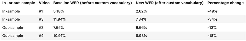
The baseline WER (before using custom vocabularies) is 5.18%.
The WER (after using custom vocabularies) is 2.62%.
The percentage change in WER score is -49.4%.

Processing video #3
The baseline WER (before using custom vocabularies) is 11.94%.
The WER (after using custom vocabularies) is 7.84%.
The percentage change in WER score is -34.4%.

To calculate our metrics for the out-sample videos (the videos that Amazon Transcribe hasn’t seen before), enter the following code:

===== Out-sample videos =====
Processing video #2
The baseline WER (before using custom vocabularies) is 7.55%.
The WER (after using custom vocabularies) is 6.56%.
The percentage change in WER score is -13.1%.

Processing video #4
The baseline WER (before using custom vocabularies) is 10.91%.
The WER (after using custom vocabularies) is 8.98%.
The percentage change in WER score is -17.6%.

Reviewing the results

The following table summarizes the changes in WER scores.

If we consider absolute WER scores, the initial WER of 5.18%, for instance, might be sufficiently low for some use cases—that’s only around 1 in 20 words that are mis-transcribed! However, this rate can be insufficient for other purposes, because domain-specific terms are often the least common words spoken (relative to frequent words such as “to,” “and,” or “I”) but the most commonly mis-transcribed. For applications like search engine optimization (SEO) and video organization by topic, you may want to ensure that these technical terms are transcribed correctly. In this section, we look at how our custom vocabulary impacted the transcription rates of several important technical terms.

Metrics for specific technical terms

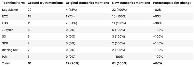
For this post, ground truth refers to the true transcript that was transcribed by hand, original transcript refers to the transcription before applying the custom vocabulary, and new transcript refers to the transcription after applying the custom vocabulary.

In-sample videos

The following table shows the transcription rates for video 1.

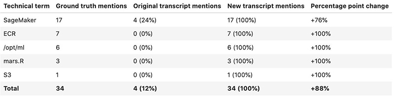
The following table shows the transcription rates for video 3.
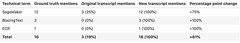
Out-sample videos

The following table shows the transcription rates for video 2.

The following table shows the transcription rates for video 4.

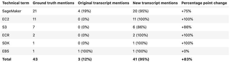
Using custom vocabularies resulted in an 80-percentage point or more increase in the number of correctly transcribed technical terms. A majority of the time, using a custom vocabulary resulted in 100% accuracy in transcribing these domain-specific terms. It looks like using custom vocabularies was worth the effort after all!

Cleaning up

To avoid incurring unnecessary charges, delete resources when not in use, including your S3 bucket, human review workflow, transcription job, and Amazon SageMaker notebook instance. For instructions, see the following, respectively:

Conclusion

In this post, you saw how you can use Amazon A2I human review workflows and Amazon Transcribe custom vocabularies to improve automated video transcriptions. This walkthrough allows you to quickly identify domain-specific terms and use these terms to build a custom vocabulary so that future mentions of term are transcribed with greater accuracy, at scale. Transcribing key technical terms correctly may be important for SEO, enabling highly specific textual queries, and grouping large quantities of video or audio files by technical terms.

The full proof-of-concept Jupyter notebook can be found in the GitHub repo. For video presentations, sample Jupyter notebooks, and more information about use cases like document processing, content moderation, sentiment analysis, object detection, text translation, and more, see Amazon Augmented AI Resources.


About the Authors

Jasper Huang is a Technical Writer Intern at AWS and a student at the University of Pennsylvania pursuing a BS and MS in computer science. His interests include cloud computing, machine learning, and how these technologies can be leveraged to solve interesting and complex problems. Outside of work, you can find Jasper playing tennis, hiking, or reading about emerging trends.


Talia Chopra is a Technical Writer in AWS specializing in machine learning and artificial intelligence. She works with multiple teams in AWS to create technical documentation and tutorials for customers using Amazon SageMaker, MxNet, and AutoGluon. In her free time, she enjoys meditating, studying machine learning, and taking walks in nature.

Read More

Live HDR+ and Dual Exposure Controls on Pixel 4 and 4a

Posted by Jiawen Chen and Sam Hasinoff, Software Engineers, Google Research

High dynamic range (HDR) imaging is a method for capturing scenes with a wide range of brightness, from deep shadows to bright highlights. On Pixel phones, the engine behind HDR imaging is HDR+ burst photography, which involves capturing a rapid burst of deliberately underexposed images, combining them, and rendering them in a way that preserves detail across the range of tones. Until recently, one challenge with HDR+ was that it could not be computed in real time (i.e., at 30 frames per second), which prevented the viewfinder from matching the final result. For example, bright white skies in the viewfinder might appear blue in the HDR+ result.

Starting with Pixel 4 and 4a, we have improved the viewfinder using a machine-learning-based approximation to HDR+, which we call Live HDR+. This provides a real-time preview of the final result, making HDR imaging more predictable. We also created dual exposure controls, which generalize the classic “exposure compensation” slider into two controls for separately adjusting the rendition of shadows and highlights. Together, Live HDR+ and dual exposure controls provide HDR imaging with real-time creative control.

Live HDR+ on Pixel 4 and 4a helps the user compose their shot with a WYSIWYG viewfinder that closely resembles the final result. You can see individual images here. Photos courtesy of Florian Kainz.

The HDR+ Look
When the user presses the shutter in the Pixel camera app, it captures 3-15 underexposed images. These images are aligned and merged to reduce noise in the shadows, producing a 14-bit intermediate “linear RGB image” with pixel values proportional to the scene brightness. What gives HDR+ images their signature look is the “tone mapping” of this image, reducing the range to 8 bits and making it suitable for display.

Consider the backlit photo of a motorcyclist, below. While the linear RGB image contains detail in both the dark motorcycle and bright sky, the dynamic range is too high to see it. The simplest method to reveal more detail is to apply a “global curve”, remapping all pixels with a particular brightness to some new value. However, for an HDR scene with details in both shadows and highlights, no single curve is satisfactory.

Different ways to tone-map a linear RGB image. (a) The original, “un-tone-mapped” image. (b) Global curve optimizing for the sky. (c) Global curve optimizing for the subject. (d) HDR+, which preserves details everywhere. In the 2D histogram, brighter areas indicate where more pixels of a given input brightness are mapped to the same output. The overlapping shapes show that the relationship cannot be modeled using a single curve. Photo courtesy of Nicholas Wilson.

In contrast to applying a single curve, HDR+ uses a local tone mapping algorithm to ensure that the final result contains detail everywhere, while keeping edges and textures looking natural. Effectively, this applies a different curve to different regions, depending on factors such as overall brightness, local texture, and amount of noise. Unfortunately, HDR+ is too slow to run live in the viewfinder, requiring an alternative approach for Live HDR+.

Local Curve Approximation for Live HDR+
Using a single tone curve does not produce a satisfying result for the entire image — but how about for a small region? Consider the small red patch in the figure below. Although the patch includes both shadows and highlights, the relationship between input and output brightness follows a smooth curve. Furthermore, the curve varies gradually. For the blue patch, shifted ten pixels to the right, both the image content and curve are similar. But while the curve approximation works well for small patches, it breaks down for larger patches. For the larger yellow patch, the input/output relationship is more complicated, and not well approximated by a single curve.

(a) Input and HDR+ result. (b) The effect of HDR+ on a small patch (red) is approximately a smooth curve. (c) The relationship is nearly identical for the nearby blue patch. (d) However, if the patch is too big, a single curve will no longer provide a good fit.

To address this challenge, we divide the input image into “tiles” of size roughly equal to the red patch in the figure above, and approximate HDR+ using a curve for each tile. Since these curves vary gradually, blending between curves is a good way to approximate the optimal curve at any pixel. To render a pixel we apply the curves from each of the four nearest tiles, then blend the results according to the distances to the respective tile centers.

Compared to HDR+, this algorithm is particularly well suited for GPUs. Since the tone mapping of each pixel can be computed independently, the algorithm can also be parallelized. Moreover, the representation is memory-efficient: only a small number of tiles is enough to represent HDR+ local tone mapping for the viewfinder.

To compute local curves, we use a machine learning algorithm called HDRnet, a deep neural network that predicts, from a linear image, per-tile curves that approximate the HDR+ look of that image. It’s also fast, due to its compact architecture and the way that low-resolution input images can be used to predict the curves for the high-resolution viewfinder. We train HDRnet on thousands of images to ensure it works well on all kinds of scenes.

HDRnet vs. HDR+ on a challenging scene with extreme brights and darks. The results are very similar at viewfinder resolution. Photo courtesy of Nicholas Wilson.

Dual Exposure Controls
HDR+ is designed to produce pleasing HDR images automatically, without the need for manual controls or post-processing. But sometimes the HDR+ rendition may not match the photographer’s artistic vision. While image editing tools are a partial remedy, HDR images can be challenging to edit, because some decisions are effectively baked into the final JPG. To maximize latitude for editing, it’s possible to save RAW images for each shot (an option in the app). However, this process takes the photographer out of the moment and requires expertise with RAW editing tools as well as additional storage.

Another approach to artistic control is to provide it live in the viewfinder. Many photographers are familiar with the exposure compensation slider, which brightens or darkens the image. But overall brightness is not expressive enough for HDR photography. At a minimum two controls are needed in order to control the highlights and shadows separately.

To address this, we introduce dual exposure controls. When the user taps on the Live HDR+ viewfinder, two sliders appear. The “Brightness” slider works like traditional exposure compensation, changing the overall exposure. This slider is used to recover more detail in bright skies, or intentionally blow out the background and make the subject more visible. The “Shadows” slider affects only dark areas — it operates by changing the tone mapping, not the exposure. This slider is most useful for high-contrast scenes, letting the user boost shadows to reveal details, or suppress them to create a silhouette.

Screen capture of dual exposure controls in action on an outdoor HDR scene with HDR+ results below. You can see individual images here. Photos courtesy of Florian Kainz.

Here are some of the dramatic renditions we were able to achieve using dual exposure controls.

Different renditions using Dual Exposure Controls. You can see individual images here. Photo credits: Jiawen Chen, Florian Kainz, Alexander Schiffhauer.

Dual Exposure Controls gives you the flexibility to capture dramatically different versions of the same subject. They are not limited to tough HDR scenes, so don’t be afraid to experiment with different subjects and lighting. You may be surprised at how much these sliders will change how you shoot!

Acknowledgements
Live HDR+ and Dual Exposure Controls is the result of a collaboration between Google Research, Android, Hardware, and UX Design teams. Key contributors include: Francois Bleibel, Sean Callanan, Yulun Chang, Eric Chen, Michelle Chen, Kourosh Derakshan, Ryan Geiss, Zhijun He, Joy Hsu, Liz Koh, Marc Levoy, Chia-Kai Liang, Diane Liang, Timothy Lin, Gaurav Malik, Hossein Mohtasham, Nandini Mukherjee, Sushil Nath, Gabriel Nava, Karl Rasche, YiChang Shih, Daniel Solomon, Gary Sun, Kelly Tsai, Sung-fang Tsai, Ted Tsai, Ruben Velarde, Lida Wang, Tianfan Xue, Junlan Yang.

Read More

Train your TensorFlow model on Google Cloud using TensorFlow Cloud

Posted by Jonah Kohn and Pavithra Vijay, Software Engineers at Google

TensorFlow Cloud is a python package that provides APIs for a seamless transition from debugging and training your TensorFlow code in a local environment to distributed training in Google Cloud. It simplifies the process of training models on the cloud into a single, simple function call, requiring minimal setup and almost zero changes to your model. TensorFlow Cloud handles cloud-specific tasks such as creating VM instances and distribution strategies for your models automatically. This article demonstrates common use cases for TensorFlow Cloud, and a few best practices.

We will walk through classifying dog breed images provided by the stanford_dogs dataset. To make this easy, we will use transfer learning with ResNet50 trained on ImageNet weights. Please find the code from this post here on the TensorFlow Cloud repository.

Setup

Install TensorFlow Cloud using pip install tensorflow_cloud. Let’s start the python script for our classification task by adding the required imports.

import datetime
import os

import matplotlib.pyplot as plt
import numpy as np
import tensorflow as tf
import tensorflow_cloud as tfc
import tensorflow_datasets as tfds

from tensorflow import keras
from tensorflow.keras import layers
from tensorflow.keras.models import Model

Google Cloud Configuration

TensorFlow Cloud runs your training job on Google Cloud using AI Platform services behind the scenes. If you are new to GCP, then please follow the setup steps in this section to create and configure your first Google Cloud Project. If you’re new to using the Cloud, first-time setup and configuration will involve a little learning and work. The good news is that after the setup, you won’t need to make any changes to your TensorFlow code to run it on the cloud!

  1. Create a GCP Project
  2. Enable AI Platform Services
  3. Create a Service Account
  4. Download an authorization key
  5. Create a Google Cloud Storage Bucket

GCP Project

A Google Cloud project includes a collection of cloud resources such as a set of users, a set of APIs, billing, authentication, and monitoring. To create a project, follow this guide. Run the commands in this section on your terminal.

export PROJECT_ID=<your-project-id>
gcloud config set project $PROJECT_ID

AI Platform Services

Please make sure to enable AI Platform Services for your GCP project by entering your project ID in this drop-down menu.

Service Account and Key

Create a service account for your new GCP project. A service account is an account used by an application or a virtual machine instance, and is used by Cloud applications to make authorized API calls.

export SA_NAME=<your-sa-name&rt;
gcloud iam service-accounts create $SA_NAME
gcloud projects add-iam-policy-binding $PROJECT_ID
--member serviceAccount:$SA_NAME@$PROJECT_ID.iam.gserviceaccount.com
--role 'roles/editor'

Next, we will need an authentication key for the service account. This authentication key is a means to ensure that only those authorized to work on your project will use your GCP resources. Create an authentication key as follows:

gcloud iam service-accounts keys create ~/key.json --iam-account $SA_NAME@$PROJECT_ID.iam.gserviceaccount.com

Create the GOOGLE_APPLICATION_CREDENTIALS environment variable.

export GOOGLE_APPLICATION_CREDENTIALS=~/key.json

Cloud Storage Bucket

If you already have a designated storage bucket, enter your bucket name as shown below. Otherwise, create a Google Cloud storage bucket following this guide. TensorFlow Cloud uses Google Cloud Build for building and publishing a docker image, as well as for storing auxiliary data such as model checkpoints and training logs.

GCP_BUCKET = "your-bucket-name"

Keras Model Creation

The model creation workflow for TensorFlow Cloud is identical to building and training a TF Keras model locally.

Resources

We’ll begin by loading the stanford_dogs dataset for categorizing dog breeds. This is available as part of the tensorflow-datasets package. If you have a large dataset, we recommend that you host it on GCS for better performance.

(ds_train, ds_test), metadata = tfds.load(
"stanford_dogs",
split=["train", "test"],
shuffle_files=True,
with_info=True,
as_supervised=True,
)

NUM_CLASSES = metadata.features["label"].num_classes

Let’s visualize the dataset:

print("Number of training samples: %d" % tf.data.experimental.cardinality(ds_train))
print("Number of test samples: %d" % tf.data.experimental.cardinality(ds_test))
print("Number of classes: %d" % NUM_CLASSES)

Number of training samples: 12000 Number of test samples: 8580 Number of classes: 120

plt.figure(figsize=(10, 10))
for i, (image, label) in enumerate(ds_train.take(9)):
ax = plt.subplot(3, 3, i + 1)
plt.imshow(image)
plt.title(int(label))
plt.axis("off")

Preprocessing

We will resize and batch the data.

IMG_SIZE = 224
BATCH_SIZE = 64
BUFFER_SIZE = 2

size = (IMG_SIZE, IMG_SIZE)
ds_train = ds_train.map(lambda image, label: (tf.image.resize(image, size), label))
ds_test = ds_test.map(lambda image, label: (tf.image.resize(image, size), label))

def input_preprocess(image, label):
image = tf.keras.applications.resnet50.preprocess_input(image)
return image, label

Configure the input pipeline for performance

Now we will configure the input pipeline for performance. Note that we are using parallel calls and prefetching so that I/O doesn’t become blocking while your model is training. You can learn more about configuring input pipelines for performance in this guide.

ds_train = ds_train.map(
input_preprocess, num_parallel_calls=tf.data.experimental.AUTOTUNE
)

ds_train = ds_train.batch(batch_size=BATCH_SIZE, drop_remainder=True)
ds_train = ds_train.prefetch(tf.data.experimental.AUTOTUNE)

ds_test = ds_test.map(input_preprocess)
ds_test = ds_test.batch(batch_size=BATCH_SIZE, drop_remainder=True)

Build the model

We will be loading ResNet50 with weights trained on ImageNet, while using include_top=False in order to reshape the model for our task.

inputs = tf.keras.layers.Input(shape=(IMG_SIZE, IMG_SIZE, 3))
base_model = tf.keras.applications.ResNet50(
weights="imagenet", include_top=False, input_tensor=inputs
)
x = tf.keras.layers.GlobalAveragePooling2D()(base_model.output)
x = tf.keras.layers.Dropout(0.5)(x)
outputs = tf.keras.layers.Dense(NUM_CLASSES)(x)

model = tf.keras.Model(inputs, outputs)

We will freeze all layers in the base model at their current weights, allowing the additional layers we added to be trained.

base_model.trainable = False

Keras Callbacks can be used easily on TensorFlow Cloud as long as the storage destination is within your Cloud Storage Bucket. For this example, we will use the ModelCheckpoint callback to save the model at various stages of training, Tensorboard callback to visualize the model and its progress, and the Early Stopping callback to automatically determine the optimal number of epochs for training.

MODEL_PATH = "resnet-dogs"
checkpoint_path = os.path.join("gs://", GCP_BUCKET, MODEL_PATH, "save_at_{epoch}")
tensorboard_path = os.path.join(
"gs://", GCP_BUCKET, "logs", datetime.datetime.now().strftime("%Y%m%d-%H%M%S")
)
callbacks = [
tf.keras.callbacks.ModelCheckpoint(checkpoint_path),
tf.keras.callbacks.TensorBoard(log_dir=tensorboard_path, histogram_freq=1),
tf.keras.callbacks.EarlyStopping(monitor="val_loss", patience=3),
]

Compile the model

optimizer = tf.keras.optimizers.Adam(learning_rate=1e-2)
model.compile(
optimizer=optimizer,
loss=tf.keras.losses.SparseCategoricalCrossentropy(from_logits=True),
metrics=["accuracy"],
)

Debug the model locally

We’ll train the model in a local environment first in order to ensure that the code works properly before sending the job to GCP. We will use tfc.remote() to determine whether the code should be executed locally or on the cloud. Choosing a smaller number of epochs than intended for the full training job will help verify that the model is working properly without overloading your local machine.

if tfc.remote():
epochs = 500
train_data = ds_train
test_data = ds_test
else:
epochs = 1
train_data = ds_train.take(5)
test_data = ds_test.take(5)
callbacks = None

model.fit(
train_data, epochs=epochs, callbacks=callbacks, validation_data=test_data, verbose=2
)
if tfc.remote():
SAVE_PATH = os.path.join("gs://", GCP_BUCKET, MODEL_PATH)
model.save(SAVE_PATH)

Model Training on Google Cloud

To train on GCP, populate the example code with your GCP project settings, then simply call tfc.run() from within your code. The API is simple with intelligent defaults for all the parameters. Again, we don’t need to worry about cloud specific tasks such as creating VM instances and distribution strategies when using TensorFlow Cloud. In order, the API will:

  • Make your python script/notebook cloud and distribution ready.
  • Convert it into a docker image with required dependencies.
  • Run the training job on a GCP cluster.
  • Stream relevant logs and store checkpoints.

The run() API provides significant flexibility for use, such as giving users the ability to specify custom cluster configuration, custom docker images. For a full list of parameters that can be used to call run(), see the TensorFlow Cloud readme.
Create a requirements.txt file with a list of python packages that your model depends on. By default, TensorFlow Cloud includes TensorFlow and its dependencies as part of the default docker image, so there’s no need to include these. Please create requirements.txt in the same directory as your python file. requirements.txt contents for this example are:

tensorflow-datasets
matplotlib

By default, the run API takes care of wrapping your model code in a TensorFlow distribution strategy based on the cluster configuration you have provided. In this example, we are using a single node multi-gpu configuration. So, your model code will be wrapped in a TensorFlow `MirroredStrategy` instance automatically.
Call run() in order to begin training on cloud. Once your job has been submitted, you will be provided a link to the cloud job. To monitor the training logs, follow the link and select ‘View logs’ to view the training progress information.

tfc.run(
requirements_txt="requirements.txt",
distribution_strategy="auto",
chief_config=tfc.MachineConfig(
cpu_cores=8,
memory=30,
accelerator_type=tfc.AcceleratorType.NVIDIA_TESLA_T4,
accelerator_count=2,
),
docker_image_bucket_name=GCP_BUCKET,
)

Visualize the model using TensorBoard

Here, we are loading the Tensorboard logs from our GCS bucket to evaluate model performance and history.

tensorboard dev upload --logdir "gs://your-bucket-name/logs" --name "ResNet Dogs"

Evaluate the model

After training, we can load the model that’s been stored in our GCS bucket, and evaluate its performance.

if tfc.remote():
model = tf.keras.models.load_model(SAVE_PATH)
model.evaluate(test_data)

Next steps

This article introduced TensorFlow Cloud, a python package that simplifies the process of training models on the cloud using multiple GPUs/TPUs into a single function, with zero code changes to your model. You can find the complete code from this article here. As a next step, you can find this code example and many others on the TensorFlow Cloud repository.Read More

Teen’s Gambit: 15-Year-Old Chess Master Puts Blundering Laptop in Check with Jetson Platform

Only 846 people in the world hold the title of Woman International Master of chess. Evelyn Zhu, age 15, is one of them.

A rising high school junior in Long Island, outside New York City, Zhu began playing chess competitively at the age of seven and has worked her way up to being one of the top players of her age.

Before COVID-19 limited in-person gatherings, Zhu typically spent two to three hours a day practicing online for an upcoming tournament — if only her laptop could keep up.

Chess engines like Leela Chess Zero — Zhu’s go-to practice partner, which recently beat all others at the 17th season of the Top Chess Engine Championship — use artificial neural network algorithms to mimic the human brain and make moves.

It takes a lot of processing power to take full advantage of such algorithms, so Zhu’s two-year-old laptop would often crash from overheating.

Zhu turned to the NVIDIA Jetson Xavier NX module to solve the issue. She connected the module to her laptop with a MicroUSB-to-USB cable and launched the engine on it. The engine ran smoothly. She also noted that doing the same with the NVIDIA Jetson AGX Xavier module doubled the speed at which the engine analyzed chess positions.

This solution is game-changing, said Zhu, as running Leela Chess Zero on her laptop allows her to improve her skills even while on the go.

AI-based chess engines allow players like Zhu to perform opening preparation, the process of figuring out new lines of moves to be made during the beginning stage of the game. Engines also help with game analysis, as they point out subtle mistakes that a player makes during gameplay.

Opening New Moves Between Chess and Computer Science

“My favorite thing about chess is the peace that comes from being deep in your thoughts when playing or studying a game,” said Zhu. “And getting to meet friends at various tournaments.”

One of her favorite memories is from the 2020 U.S. Team East Tournament, the last she competed at before the COVID-19 outbreak. Instead of the usual competition where one wins or loses as an individual, this was a tournament where players scored points for their teams by winning individual matches.

Zhu’s squad, comprising three other girls around her age, placed second out of 318 teams of all ages.

“Nobody expected that, especially because we were a young all-girls team,” she said. “It was so memorable.”

Besides chess, Zhu has a passion for computer science and hopes to study it in college.

“What excites me most about CS is that it’s so futuristic,” she said. “It seems like we’re making progress in AI on a daily basis, and I really think that it’s the route to advancing society.”

Working with the Jetson platform has opened up a pathway for Zhu to combine her passions for chess and AI. After she posted online instructions on how she supercharged her crashing laptop with NVIDIA technology, Zhu heard from people all around the world.

Her post even sparked discussion of chess in the context of AI, she said, showing her that there’s a global community interested in the topic.

Find out more about Zhu’s chess and tech endeavors.

Learn more about the Jetson platform.

The post Teen’s Gambit: 15-Year-Old Chess Master Puts Blundering Laptop in Check with Jetson Platform appeared first on The Official NVIDIA Blog.

Read More