Monthly Archives: August 2020

We’re extremely excited to share the Deep Graph Knowledge Embedding Library (DGL-KE), a knowledge graph (KG) embeddings library built on top of the Deep Graph Library (DGL). DGL is an easy-to-use, high-performance, scalable Python library for deep learning on graphs. You can now create embeddings for large KGs containing billions of nodes and edges two-to-five times faster than competing techniques.

For example, DGL-KE has created embeddings on top of the Drug Repurposing Knowledge Graph (DRKG) to show which drugs can be repurposed to fight COVID-19. These embeddings can be used to predict the likelihood of a drug’s ability to treat a disease or bind to a protein associated with the disease.

In this post, we focus on creating knowledge graph embeddings (KGE) using the Kensho Derived Wikimedia Dataset (KDWD). You can use those embeddings to find similar nodes and predict new relations. For example, in natural language processing (NLP) and information retrieval use cases, you can parse a new query and transform it syntactically into a triplet (subject, predicate, object). Upon adding new triplets to a KG, you can augment nodes and relations by classifying nodes and inferring relations based on the existing KG embeddings. This helps guide and find the intent for a chatbot application, for example, and provide the right FAQ or information to a customer.

Knowledge graph

A knowledge graph is a structured representation of facts, consisting of entities, relationships, and semantic descriptions purposely built for a given domain or application. They are also known as heterogenous graphs, where there are multiple entity types and relation types. The information stored in a KG is often specified in triplets, which contain three elements: head, relation, and tail ([h,r,t]). Heads and tails are also known as entities. The union of triplets is also known as statements.

KGs allow you to model your information very intuitively and expressively, giving you the ability to integrate data easily. For example, you can use Amazon Neptune to build an identity graph powering your customer 360 or Know Your Customer application commonly found in financial services. In healthcare and life sciences, where data is usually sparse, KGs can integrate and harmonize data from different silos using taxonomy and vocabularies. In e-commerce and telco, KGs are commonly used in question answering, chatbots, and recommender systems. Fore more information on using Amazon Neptune for your use case, visit the Amazon Neptune homepage.

Knowledge graph embeddings

Knowledge graph embeddings are low-dimensional representations of the entities and relations in a knowledge graph. They generalize information of the semantic and local structure for a given node.

Many popular KGE models exist, such as TransE, TransR, RESCAL, DistMult, ComplEx, and RotatE.

Each model has a different score function that measures the distance of two associated entities by their relation. The general intuition is that entities connected by a relation are closed to each other, whereas the entities that aren’t connected are far apart in the vector space.

The scoring functions for the models currently supported by DGL-KE are as follows:

Wikimedia dataset

In our use case, we use the Kensho Derived Wikimedia Dataset (KDWD). You can find the notebook example and code in the DGL-KE GitHub repo.

The combination of Wikipedia and Wikidata is composed of three data layers:

• Base – Contains the English Wikipedia corpus
• Middle – Identifies which text spans are links and annotates the corpus
• Top – Connects Wikipedia links to items in the Wikidata KG

The following diagram illustrates these data layers.

The KDWD contains the following:

• 2,315,761,359 tokens
• 121,835,453 page links
• 5,343,564 Wikipedia pages
• 51,450,317 Wikidata items
• 141,206,854 Wikidata statements

The following code is an example of the entity.txt file:

ID	Label		Description
1	Universe	totality of space and all contents
2	Earth		third planet from the Sun in the Solar System
3	life		matter capable of extracting energy from the environment for replication

Before you can create your embeddings, you need to pre-process the data. DGL-KE gives you the ability to compute embeddings using two formats.

In raw user-defined knowledge graphs, you provide the triplets; the entities and relations can be arbitrary strings. The dataloader automatically generates the ID mappings.

The following table from Train User-Defined Knowledge Graphs shows an example of triplets.

In user-defined knowledge graphs, you also provide the ID mapping for entities and relations (the triplets should only contain these IDs). The IDs start from 0 and are continuous. The following table from Train User-Defined Knowledge Graphs shows an example of mapping and triplets files.

For more information, see DGL-KE Command Lines.

Although the dataset KDWD provides dictionaries, we can’t use it for our use case because the index doesn’t start with 0 and the index values aren’t continuous. We preprocess our data and use the raw format to generate our embeddings. After merging and cleaning the data, we end up with a KG with the following properties:

• 39,569,815 entities
• 1,213 relations
• Approximately 120 million statements

The following code is an example of the triplets.

Head			Relation			Tail
Eiksteinen      	located in the administrative…	Rogaland
Trivellona marlowi     instance of     		taxon
Acta Numerica   	main subject    		mathematical analysis
Günther Neukirchner    given name      		Günther
Ruth Pointer    	given name      		Ruth

DGL-KE has many different training modes. CPU, GPU, mix-CPU-GPU mode, and distributed training are all supported options, depending on your dataset and training requirements. For our use case, we use mix mode to generate our embeddings. If you can contain all the data in GPU memory, GPU is the preferred method. Because we’re training on a large KG, we use mix mode to get a larger pool of CPU- and GPU-based memory and still benefit from GPU for accelerated training.

We create our embeddings with the dgl-ke command line. See the following code:

!DGLBACKEND=pytorch dglke_train 
--model_name TransE_l2 
--batch_size 1000 
--neg_sample_size 200 
 --hidden_dim 400 
--gamma 19.9 
--lr 0.25 
--max_step 24000 
--log_interval 100 
--batch_size_eval 16 
-adv 
--regularization_coef 1.00E-09 
--test 
--gpu 0 1 2 3 
--mix_cpu_gpu 
--save_path ./wikimedia 
--data_path ./data/wikimedia/ 
--format raw_udd_hrt 
--data_files train.txt valid.txt test.txt 
--neg_sample_size_eval 10000

For more information about the DGL-KE arguments, see the DGL-KE website.

We trained our KG of about 40 million entities and 1,200 relations and approximately 120 million statements on a p3.8xl in about 7 minutes.

We evaluate our model by entering the following code:

!DGLBACKEND=pytorch dglke_eval --dataset wikimedia --model_name TransE_l2 
--neg_sample_size 200 --hidden_dim 400 --gamma 19.9 
--batch_size_eval 16 --gpu 0 1 2 3  --model_path ./wikimedia/TransE_l2_wikimedia_0/ 
--data_path ./data/wikimedia/ --format raw_udd_hrt --data_files train.txt valid.txt test.txt --neg_sample_size_eval 10000 --no_eval_filter

The following code is the output:

-------------- Test result --------------
Test average MRR: 0.4159753346227368
Test average MR: 1001.1689418833716
Test average HITS@1: 0.3540242971873324
Test average HITS@3: 0.45541123141672746
Test average HITS@10: 0.5213350742247359
-----------------------------------------

DGL-KE allows you to perform KG downstream tasks by using any combinations of [h,r,t].

In the following example, we find similar node entities for two people by creating a head.list file with the following entries:

head.list
Jeff Bezos
Barack Obama

DGL-KE provides functions to perform offline inference on entities and relations.

To find similar node entities from our head.list, we enter the following code:

!DGLBACKEND=pytorch dglke_emb_sim 
--format 'l_*' --data_files /home/ec2-user/SageMaker/DGL-Neptune/notebooks/data/wikimedia/head.list 
--mfile ./data/wikimedia/entities.tsv 
--emb_file ./wikimedia/TransE_l2_wikimedia_1/wikimedia_TransE_l2_entity.npy 
--raw_data --gpu 0 
--exec_mode 'batch_left' 
--sim_func 'cosine' --topK 5

The following code is the output:

resulst.tsv
head tail score
Jeff Bezos Jeff Bezos 1.0
Jeff Bezos Aga Khan IV 0.8602205514907837
Jeff Bezos Alisher Usmanov 0.8584005236625671
Jeff Bezos Klaus Tschira 0.8512368202209473
Jeff Bezos Bill Gates 0.8441287875175476
Barack Obama Barack Obama 1.0
Barack Obama Donald Trump 0.9529082179069519
Barack Obama George W. Bush 0.9426612854003906
Barack Obama Harry S. Truman 0.9414601922035217
Barack Obama Ronald Reagan 0.9393566250801086

Interestingly, all the nodes similar to Jeff Bezos describe tech tycoons. Barack Obama’s similar nodes show former and current presidents of the US.

Conclusion

Graphs can be found in many domains, such as chemistry, biology, financial services, and social networks, and allow us to represent complex concepts intuitively using entities and relations. Graphs can be homogeneous or heterogeneous, where you have many types of entities and relations.

Knowledge graph embeddings give you powerful methods to encode semantic and local structure information for a given node, and you can also use them as input for machine learning and deep learning models. DGL-KE supports popular embedding models and allows you to compute those embeddings on CPU or GPU at scale two-to-five times faster than other techniques.

We’re excited to see how you use graph embeddings on your existing KGs or new machine learning problems. For more information about the library, see the DGL-KE GitHub repo. For instructions on using Wikimedia KG embeddings in your KG, see the DGL-KE notebook example.

About the Authors

Phi Nguyen is a solution architect at AWS helping customers with their cloud journey with a special focus on data lake, analytics, semantics technologies and machine learning. In his spare time, you can find him biking to work, coaching his son’s soccer team or enjoying nature walk with his family.

Xiang Song is an Applied Scientist with the AWS Shanghai AI Lab. He got his Bachelor’s degree in Software Engineer and Ph.D’s in Operating System and Architecture from Fudan University. His research interests include building machine learning systems and graph neural network for real world applications.

Read More

Are you bored of the same old board games? Tired of going through the motions with charades week after week? In need of a fun and exciting way to mix up game night? Well we have a solution for you!

From the makers of AWS DeepLens, Guess My Drawing with DeepLens is a do-it-yourself recipe for building your very own Machine Learning (ML)-enabled Pictionary-style game! In this post, you learn how to harness the power of AWS DeepLens, the AWS programmable video camera for developers to learn ML, and Amazon Alexa, the Amazon cloud-based voice service.

You start by learning to deploy a trained model to AWS DeepLens that can recognize sketches drawn on a whiteboard and pair it with an Alexa skill that serves as the official scorekeeper.

When your recipe is complete, the fun begins!

Solution overview

Guess My Drawing with AWS DeepLens uses Alexa to host a multi-player drawing challenge game. To get started, gather your game supplies mentioned in the Prerequisites section.

To initiate gameplay, simply say, “Alexa, play Guess My Drawing with DeepLens.” Alexa explains the game rules and asks how many players are playing the game. The players decide the turn order.

Alexa provides each player with a common word. For example, Alexa may say, “Your object to draw is bowtie.” The player has 12 seconds to draw it on a whiteboard without writing letters or words.

When time runs out, the player stops drawing and asks Alexa to share the results. The ML model running on AWS DeepLens predicts the object that you drew. If the object matches with what Alexa asks, Alexa awards 10 points. If DeepLens can’t correctly guess the drawing or the player takes more than 12 seconds to draw, no points are earned.

Alexa prompts the next participant with their word, repeating until all participants have taken a turn. After each round, Alexa provides a score update. The game ends after five rounds, and whoever has the highest score wins the game!

The following diagram shows the architecture of our solution.

This tutorial includes the following steps:

1. Create an AWS DeepLens inference AWS Lambda function to isolate the drawing area and feed each camera frame into the model to generate predictions on the sketches.
2. Deploy a pre-trained trained model included in this post to AWS DeepLens to perform image classification.
3. Create an AWS IoT Core rule to send the results to Amazon Kinesis Data Streams.
4. Create a custom Alexa skill with a different Lambda function to retrieve the detected objects from the Kinesis data stream and have Alexa verbalize the result to you.

Prerequisites

Before you begin this tutorial, make sure you have the following prerequisites:

• An AWS account
• An AWS DeepLens device, available from the following:
  • Amazon.com (US)
  • Amazon.ca (Canada)
  • Amazon.co.jp (Japan)
  • Amazon.de (Germany)
  • Amazon.co.uk (UK)
  • Amazon.fr (France)
  • Amazon.es (Spain)
  • Amazon.it (Italy)
• An Amazon Alexa device
• A whiteboard or paper pad (unlined)
• A marker or writing utensil

Creating an AWS DeepLens inference Lambda function

In this section, you create an inference function that you deploy to AWS DeepLens. The inference function isolates the drawing area, optimizes the model to run on AWS DeepLens, and feeds each camera frame into the model to generate predictions.

To create your function, complete the following steps:

1. Download aws-deeplens-pictionary-lambda.zip.
2. On the Lambda console, choose Create function.
3. Choose Author from scratch and choose the following options:
   2. For Runtime, choose Python 2.7.
   3. For Choose or create an execution role, choose Use an existing role.
   4. For Existing role, enter service-role/AWSDeepLensLambdaRole.
4. After you create the function, go to the Function code
5. From the Actions drop-down menu in Function code, choose Upload a .zip file.
6. Upload the aws-deeplens-pictionary-lambda.zip file you downloaded earlier.
7. Choose Save.
8. From the Actions drop-down menu, choose Publish new version.
9. Enter a version number and choose Publish.

Publishing the function makes it available on the AWS DeepLens console so you can add it to your custom project.

Understanding the Lambda function

You should pay attention to the following two files:

• labels.txt – This file is for the inference function to translate the numerical result from the model into human readable labels used in our game. It contains a list of 36 objects on which the model has been trained to recognize sketches.
• lambda_function.py – This file contains the preprocessing algorithm and the function being called to generate predictions on drawings and send back results.

Because the model was trained on digital sketches with clean, white backgrounds, we have a preprocessing algorithm that helps isolate the drawing and remove any clutter in the background. You can find the algorithm to do this in the isolate_image() function inside the lambda_function.py file. In this section, we walk you through some important parts of the preprocessing algorithm.

Fisheye calibration

AWS DeepLens uses a wide-angle lens to get as much information as possible in the frame. As a result, any input frame is distorted, especially for the rectangular shape of a whiteboard. Therefore, you need to perform fisheye calibration to straighten the edges. As part of this post, we provide the calibration code to undistort your AWS DeepLens images. The following code straightens the edges and eliminates the distortion:

def undistort(frame): 
    frame_height, frame_width, _ = frame.shape
 K=np.array([[511.98828907136766, 0.0, 426.48016197546474], 
                [0.0, 513.8644747557715, 236.89875770956868], 
                [0.0, 0.0, 1.0]])
    D=np.array([[-0.10969105781526832], [0.03463562293251206], 
                [-0.2341226037892333], [0.34335682066685935]])
    DIM = (int(frame_width/3), int(frame_height/3))
    frame_resize = cv2.resize(frame, DIM)
    map1, map2 = cv2.fisheye.initUndistortRectifyMap(K, D, np.eye(3), 
                                                     K, DIM, cv2.CV_16SC2)
    undistorted_img = cv2.remap(frame_resize, map1, map2, 
                                interpolation=cv2.INTER_LINEAR, 
                                borderMode=cv2.BORDER_CONSTANT)
    return undistorted_img

The following screenshots shows the raw image captured by AWS DeepLens.

The following screenshot shows the results of the undistort function with fisheye calibration.

The next code section enhances the images to eliminate the effects caused by different lighting conditions:

enh_con = ImageEnhance.Contrast(img_colored)
contrast = 5.01
img_contrasted = enh_con.enhance(contrast)
image = img_contrasted
image = np.array(image)

The following screenshot shows the results of the contrast enhancement.

Canny Edge Detection

The next part of the preprocessing algorithm uses OpenCV’s Canny Edge Detection technique to find the edges in the image. See the following code:

# these constants are carefully picked
    MORPH = 9
    CANNY = 84
    HOUGH = 25
    img = cv2.cvtColor(image, cv2.COLOR_BGR2GRAY)
    cv2.GaussianBlur(img, (3,3), 0, img)
    # this is to recognize white on white
    kernel = cv2.getStructuringElement(cv2.MORPH_RECT,(MORPH,MORPH))
    dilated = cv2.dilate(img, kernel)
    edges = cv2.Canny(dilated, 0, CANNY, apertureSize=3)
    lines = cv2.HoughLinesP(edges, 1,  3.14/180, HOUGH)
    for line in lines[0]:
        cv2.line(edges, (line[0], line[1]), (line[2], line[3]), (255,0,0), 2, 8)

The following screenshot shows the results from applying the Canny Edge Detector.

For more information about how Canny Edge Detection works, see the Canny Edge Detection tutorial on the OpenCV website.

Finding contours

After the edges are found, you can use OpenCV’s findContours() function to extract the polygon contours from the image. This function returns a list of polygon shapes that are closed and ignores any open edges or lines. See the following code:

contours, _ = cv2.findContours(edges.copy(), cv2.RETR_EXTERNAL, cv2.CHAIN_APPROX_SIMPLE)
contours = filter(lambda cont: cv2.arcLength(cont, False) > 100, contours)
contours = filter(lambda cont: cv2.contourArea(cont) > 10000, contours)
 result = None
for idx, c in enumerate(contours):
      if len(c) < Config.min_contours:
          continue
      epsilon = Config.epsilon_start
      while True:
            approx = cv2.approxPolyDP(c, epsilon, True)
            approx = approx.reshape((len(approx), 2))
            new_approx = []
            for i in range(len(approx)):
                if 80 < approx[i][0] < 750:
                    new_approx.append(approx[i])
            approx = np.array(new_approx)
            if (len(approx) < 4):
                break
            if math.fabs(cv2.contourArea(approx)) > Config.min_area:
                if (len(approx) > 4):
                    epsilon += Config.epsilon_step
                    continue
                else:
                    # for p in approx:
                    #  cv2.circle(binary,(p[0][0],p[0][1]),8,(255,255,0),thickness=-1)
                    approx = approx.reshape((4, 2))
                    # [top-left, top-right, bottom-right, bottom-left]
                    src_rect = order_points(approx)
                    cv2.drawContours(image, c, -1, (0, 255, 255), 1)
                    cv2.line(image, (src_rect[0][0], src_rect[0][1]), (src_rect[1][0], src_rect[1][1]),
                             color=(100, 255, 100))
                    cv2.line(image, (src_rect[2][0], src_rect[2][1]), (src_rect[1][0], src_rect[1][1]),
                             color=(100, 255, 100))
                    cv2.line(image, (src_rect[2][0], src_rect[2][1]), (src_rect[3][0], src_rect[3][1]), 
                             color=(100, 255, 100))
                    cv2.line(image, (src_rect[0][0], src_rect[0][1]), (src_rect[3][0], src_rect[3][1]),
                             color=(100, 255, 100))

For more information, see Contours: Getting Started.

Perspective transformation

Finally, the preprocessing algorithm does perspective transformation to correct for any skew. The following code helps achieve perspective transformation and crop a rectangular area:

M = cv2.getPerspectiveTransform(src_rect, dst_rect)
warped = cv2.warpPerspective(image, M, (w, h))	

The following image is the input of the preprocessing algorithm.

The following image is the final result.

Performing inference

In this section, you learn how to perform inference with an ML model and send back results from AWS DeepLens.

AWS DeepLens uses the Intel OpenVino model optimizer to optimize the ML model to run on DeepLens hardware. The following code optimizes a model to run locally:

error, model_path = mo.optimize(model_name, INPUT_WIDTH, INPUT_HEIGHT)

The following code loads the model:

model = awscam.Model(model_path, {'GPU': 1})

The following code helps run the model frame-per-frame over the images from the camera:

ret, frame = awscam.getLastFrame()

Viewing the text results in the cloud is a convenient way to make sure the model is working correctly. Each AWS DeepLens device has a dedicated iot_topic automatically created to receive the inference results. The following code sends the messages from AWS DeepLens to the IoT Core console:

# Send the top k results to the IoT console via MQTT
cloud_output = {}
for obj in top_k:
    cloud_output[output_map[obj['label']]] = obj['prob']
client.publish(topic=iot_topic, payload=json.dumps(cloud_output))

Deploying the model to AWS DeepLens

In this section, you set up your AWS DeepLens device, import a pre-trained model, and deploy the model to AWS DeepLens.

Setting up your AWS DeepLens device

You first need to register your AWS DeepLens device, if you haven’t already.

After you register your device, you need to install the latest OpenCV (version 4.x) packages and Pillow libraries to enable the preprocessing algorithm in the DeepLens inference Lambda function. To do so, you need the IP address of AWS DeepLens on the local network, which is listed in the Device details section. You also need to ensure that Secure Shell (SSH) is enabled for your device. For more information about enabling SSH on your device, see View or Update Your AWS DeepLens 2019 Edition Device Settings.

Open a terminal application on your computer. SSH into your DeepLens by entering the following code into your terminal application:

ssh aws_cam@<YOUR_DEEPLENS_IP>

Then enter the following commands in the SSH terminal:

sudo su
pip install --upgrade pip
pip install opencv-python
pip install pillow

Importing the model to AWS DeepLens

For this post, you use a pre-trained model. We trained the model for 36 objects on The Quick Draw Dataset made available by Google, Inc., under the CC BY 4.0 license. For each object, we took 1,600 images for training and 400 images for testing the model from the dataset. Holding back 400 images for testing allows us to measure the accuracy of our model against images that it has never seen.

For instructions on training a model using Amazon SageMaker as the development environment, see AWS DeepLens Recipes and Amazon SageMaker: Build an Object Detection Model Using Images Labeled with Ground Truth.

To import your model, complete the following steps:

1. Download the model aws-deeplens-pictionary-game.tar.gz.
2. Create an Amazon Simple Storage Service (Amazon S3) bucket to store this model. For instructions, see How do I create an S3 Bucket?

The S3 bucket name must contain the term deeplens. The AWS DeepLens default role has permission only to access the bucket with the name containing deeplens.

3. After the bucket is created, upload aws-deeplens-pictionary-game.tar.gz to the bucket and copy the model artifact path.
4. On the AWS DeepLens console, under Resources, choose Models.
5. Choose Import model.
   
6. On the Import model to AWS DeepLens page, choose Externally trained model.
7. For Model artifact path, enter the Amazon S3 location for the model you uploaded earlier.
8. For Model name, enter a name.
9. For Model framework, choose MXNet.
10. Choose Import model.
    

Deploying the model to your AWS DeepLens device

To deploy your model, complete the following steps:

1. On the AWS DeepLens console, under Resources, choose Projects.
2. Choose Create new project.
3. Choose Create a new blank project.
4. For Project name, enter a name.
5. Choose Add model and choose the model you imported earlier.
6. Choose Add function and choose the Lambda function you created earlier.
7. Choose Create.
   
8. Select your newly created project and choose Deploy to device.
9. On the Target device page, select your device from the list.
10. On the Review and deploy page, choose Deploy.

The deployment can take up to 5 minutes to complete, depending on the speed of the network your AWS DeepLens is connected to. When the deployment is complete, you should see a green banner message that the deployment succeeded.

To verify that the project was deployed successfully, you can check the text prediction results sent to the cloud via AWS IoT Greengrass. For instructions, see Using the AWS IoT Greengrass Console to View the Output of Your Custom Trained Model (Text Output).

In addition to the text results, you can view the pose detection results overlaid on top of your AWS DeepLens live video stream. For instructions, see Viewing AWS DeepLens Output Streams.

Sending results from AWS DeepLens to a data stream

In this section, you learn how to send messages from AWS DeepLens to a Kinesis data stream by configuring an AWS IoT rule.

1. On the Kinesis console, create a new data stream.
2. For Data stream name, enter a name.
3. For Number of shards, choose 1.
4. Choose Create data stream.
   
5. On the AWS IoT console, under Act, choose Rules.
6. Choose Create to set up a rule to push MQTT messages from AWS DeepLens to the newly created data stream.
   
7. On the Create a rule page, enter a name for your rule.
8. For Rule query statement, enter the DeepLens device MQTT topic.
9. Choose Add action.
   
10. Choose Send a message to an Amazon Kinesis Stream.
11. Choose Configuration.
12. Choose the data stream you created earlier.
13. For Partition key, enter ${newuuid()}.
14. Choose Create a new role or Update role.
15. Choose Add action.
16. Choose Create rule to finish the setup.
    

Now that the rule is set up, MQTT messages are loaded into the data stream.

Amazon Kinesis Data Streams is not currently available in the AWS Free Tier, which offers a free trial for a group of AWS services. For more information about the pricing of Amazon Kinesis Data Streams, see link.

We recommend that you delete the data stream after completing the tutorial because charges occur on an active data stream even when you aren’t sending and receiving messages.

Creating an Alexa skill

In this section, you first create a Lambda function that queries a data stream and returns the sketches detected by AWS DeepLens to Alexa. Then, you create a custom Alexa skill to start playing the game.

Creating a custom skill with Lambda

To create your custom skill in Lambda, complete the following steps:

1. On the Lambda console, create a new function.

The easiest way to create an Alexa skill is to create the function from the existing blueprints or serverless app repository provided by Lambda and overwrite the code with your own.

2. For Create function, choose Browse serverless app repository.
3. For Public repositories, search for and choose alexa-skills-kit-color-expert-python.
   
4. Under Application settings, enter an application name and TopicNameParameter.
5. Choose Deploy.
6. When the application has been deployed, open the Python file.
   
7. Download the alexa-lambda-function.py file onto your computer.
8. Copy the Python code from the file and replace the sample code in the lambda_function.py file in the Function code section.

This function includes the entire game logic, reads data from the data stream, and returns the result to Alexa. Be sure to change the Region from the default (us-east-1) if you’re in a different Region. See the following code:

kinesis = boto3.client(‘kinesis’, region_name=’us-east-1′

9. Set the Timeout value to 20 seconds.

You now need to give your Lambda function IAM permissions to read data from the data stream.

10. In your Lambda function editor, choose Permissions.
11. Choose the Role name under the Execution role.

You’re directed to the IAM role editor.

12. In the editor, choose Attach policies.
13. Enter Kinesis and choose AmazonKinesisFullAccess.
14. Choose Attach policy.
    

Creating a custom skill to play the game

To create your second custom skill to start playing the game, complete the following steps:

1. Log in to the Alexa Developer Console.
2. Create a new custom Alexa skill.
3. On the Create a new skill page, for Skill name, enter a skill name
4. For Choose a model to add to your skill, choose Custom.
5. For Choose a method to host your skill’s backend resources, choose Provision your own.
6. Choose Create skill.
   
7. On the next page, choose the default template to add your skill.
8. Choose Continue with template.

After about 1–2 minutes, your skill appears on the console.

9. In the Endpoint section, enter the Amazon Resource Name (ARN) of the Lambda function created for the Alexa skill in the previous step.
   
10. Download alexa-skill-json-code.txt onto your computer.
11. Copy the code from the file and paste in the Alexa skill JSON editor to automatically configure intents and sample utterances for the custom skill.

In the Alexa architecture, intents can be thought of as distinct functions that a skill can perform. Intents can take arguments that are known here as slots.

12. Choose Save Model to apply the changes.
13. Choose Build Model.
    
14. On the Lambda console, open the Lambda function for the Alexa skill you created earlier.

You need to enable the skill by adding a trigger to the Lambda function.

15. Choose Add trigger.
16. Choose Alexa Skills Kit.
17. For Skill ID, enter the ID for the Alexa skill you created.
18. Choose Add.
    

Testing the skill

Your Alexa skill is now ready to tell you the drawings detected by AWS DeepLens. To test with an Alexa-enabled device (such as an Amazon Echo), register the device with the same email address you used to sign up for your developer account on the Amazon Developer Portal. You can invoke your skill with the wake word and your invocation name: “Alexa, Play Guess My Drawing with DeepLens.”

The language in your Alexa companion app should match with the language chosen in your developer account. Alexa considers English US and English UK to be separate languages.

Alternatively, the Test page includes a simulator that lets you test your skill without a device. For Skill testing is enabled in, choose Development. You can test your skill with the phrase, “Alexa, Play Guess My Drawing with DeepLens.”

Windows 10 users can download the free Alexa app from the Microsoft Store and interact with it from their PC.

For more information on testing your Alexa skill, see Test Your Skill. For information on viewing the logs, check Amazon CloudWatch logs for AWS Lambda.

The following diagram shows the user interaction flow of our game.

The following images show the prediction outputs of our model with the name of an object and its probability. You need to have your AWS DeepLens located in front of a rectangular-shaped whiteboard or a piece of white paper to ensure that the edges are visible in the frame.

Conclusion

In this post, you learned about the preprocessing algorithm to isolate a drawing area and how to deploy a pre-trained model onto AWS DeepLens to recognize sketches. Next, you learned how to send results from AWS IoT to Kinesis Data Streams. Finally, you learned how to create a custom Alexa skill with Lambda to retrieve the detected objects in the data stream and return the results to players via Alexa.

For other tutorials, samples, and project ideas with AWS DeepLens, see AWS DeepLens Recipes.

About the Authors

Amit Choudhary is a Senior Product Manager Technical Intern. He loves to build products that help developers learn about various machine learning techniques in a fun and hands-on manner.

Phu Nguyen is a Product Manager for AWS DeepLens. He builds products that give developers of any skill level an easy, hands-on introduction to machine learning.

Brian Nguyen is an undergraduate senior in majoring Electrical Engineering with a concentration of Digital Signal & Image Processing at University of Washington Seattle.

Hanwen Guo is an undergraduate senior majoring in Electrical Engineering with a concentration of Digital Signal & Image Processing at University of Washington Seattle.

Jack Ma is an undergraduate senior majoring in Electrical Engineering with a concentration of Embedded Systems at University of Washington Seattle.

Sairam Tabibu is pursuing a master’s degree in Electrical Engineering with an interest in machine learning/deep learning at University of Washington Seattle

Aaron Liang is pursuing a master’s degree in Electrical Engineering with an interest in software engineering at University of Washington Seattle

Read More

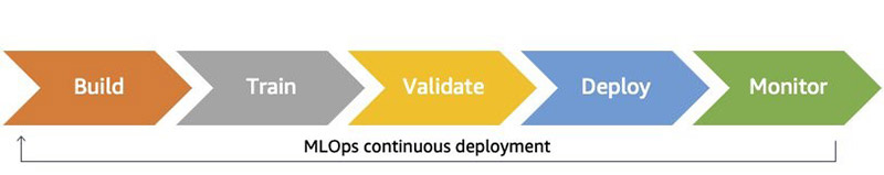
As machine learning (ML) applications become more popular, customers are looking to streamline the process for developing, deploying, and continuously improving models. To reliably increase the frequency and quality of this cycle, customers are turning to ML operations (MLOps), which is the discipline of bringing continuous delivery principles and practices to the data science team. The following diagram illustrates the continuous deployment workflow.

There are many ways to operationalizing ML. In this post, you see how to build an ML model that predicts taxi fares in New York City using Amazon SageMaker, AWS CodePipeline, and AWS CodeDeploy in a safe blue/green deployment pipeline.

Amazon SageMaker is a fully managed service that provides developers and data scientists the ability to quickly build, train, deploy, and monitor ML models. When combined with CodePipeline and CodeDeploy, it’s easy to create a fully serverless build pipeline with best practices in security and performance with lower costs.

CodePipeline is a fully managed continuous delivery service that helps you automate your release pipelines for fast and reliable application and infrastructure updates. CodePipeline automates the Build, Test, and Deploy phases of your release process every time a code change occurs, based on the release model you define.

What is blue/green deployment?

Blue/green deployment is a technique that reduces downtime and risk by running two identical production environments called Blue and Green. After you deploy a fully tested model to the Green endpoint, a fraction of traffic (for this use case, 10%) is sent to this new replacement endpoint. This continues for a period of time while there are no errors with an optional ramp up to reach 100% of traffic, at which point the Blue endpoint can be decommissioned. Green becomes live, and the process can repeat again. If any errors are detected during this process, a rollback occurs; Blue remains live and Green is decommissioned. The following diagram illustrates this architecture.

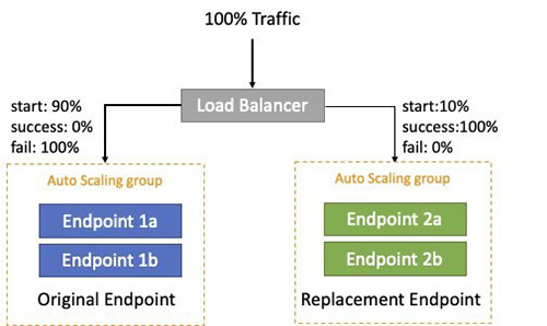
In this solution, the blue/green deployment is managed by AWS CodeDeploy with the AWS Lambda compute platform to switch between the blue/green autoscaling Amazon SageMaker endpoints.

Solution overview

For this post, you use a publicly available New York green taxi dataset to train an ML model to predict the fare amount using the Amazon SageMaker built-in XGBoost algorithm.

You automate the process of training, deploying, and monitoring the model with CodePipeline, which you orchestrate within an Amazon SageMaker notebook.

Getting started

This walkthrough uses AWS CloudFormation to create a continuous integration pipeline. You can configure this to a public or private GitHub repo with your own access token, or you can use an AWS CodeCommit repository in your environment that is cloned from the public GitHub repo.

Complete the following steps:

1. Optionally, fork a copy of the GitHub repo into your own GitHub account by choosing the fork
   1. Create a personal access token (OAuth 2) with the scopes (permissions) admin:repo_hook and repo. If you already have a token with these permissions, you can use that. You can find a list of all your personal access tokens in https://github.com/settings/tokens.
   2. Copy the access token to your clipboard. For security reasons, after you navigate off the page, you can’t see the token again. If you lose your token, you can regenerate
2. Choose Launch Stack:
   
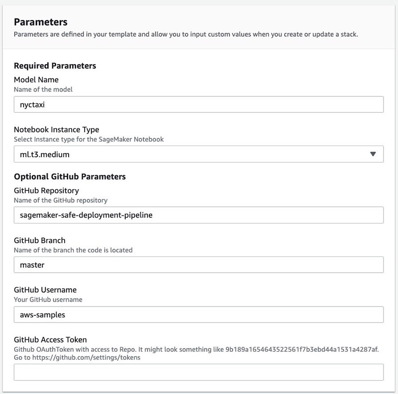
3. Enter the following parameters:
   1. Model Name – A unique name for this model (must be fewer than 15 characters)
   2. Notebook Instance Type – The Amazon SageMaker instance type (default is ml.t3.medium)
   3. GitHub Access Token – Your access token

   

4. Acknowledge that AWS CloudFormation may create additional AWS Identity and Access Management (IAM) resources.
5. Choose Create stack.

The CloudFormation template creates an Amazon SageMaker notebook and pipeline.

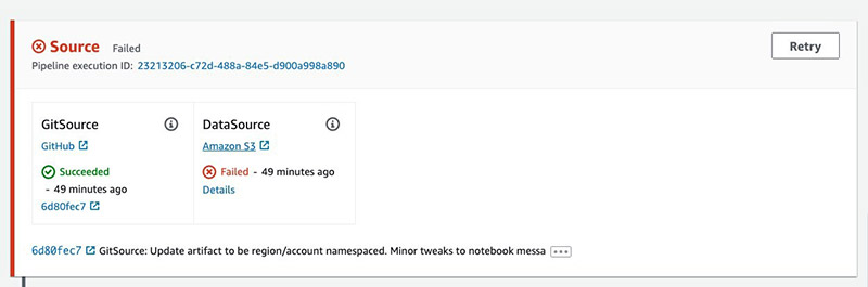
When the deployment is complete, you have a new pipeline linked to your GitHub source. It starts in a Failed state because it’s waiting on an Amazon Simple Storage Service (Amazon S3) data source.

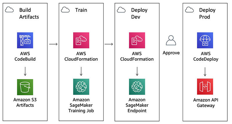
The pipeline has the following stages:

1. Build Artifacts – Run a CodeBuild job to create CloudFormation templates.
2. Train – Train an Amazon SageMaker pipeline and baseline processing job.
3. Deploy Dev – Deploys a development Amazon SageMaker endpoint.
4. Manual Approval – The user gives approval.
5. Deploy Prod – Deploys an Amazon API Gateway AWS Lambda function in front of the Amazon SageMaker endpoints using CodeDeploy for blue/green deployment and rollback.

The following diagram illustrates this workflow.

Running the pipeline

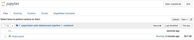
Launch the newly created Amazon SageMaker notebook in your AWS account. For more information, see Build, Train, and Deploy a Machine Learning Model.

Navigate to the notebook directory and open the notebook by choosing the mlops.ipynb link.

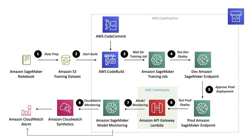
The notebook guides you through a series of steps, which we also review in this post:

1. Data Prep
2. Start Build
3. Wait for Training Job
4. Test Dev Deployment
5. Approve Prod Deployment
6. Test Prod Deployment
7. Model Monitoring
8. CloudWatch Monitoring

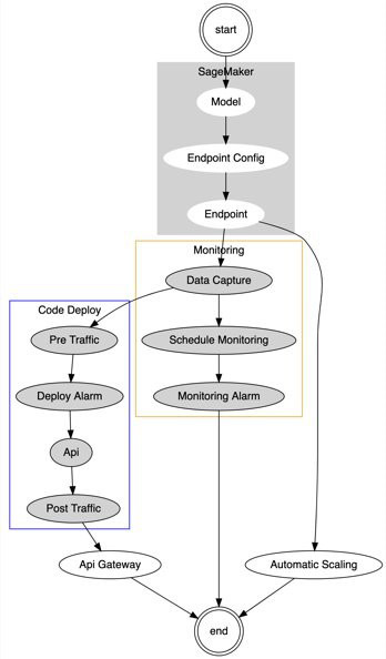
The following diagram illustrates this workflow.

Step 1: Data Prep

In this step, you download the February 2018 trips from New York green taxi trip records to a local file for input into a pandas DataFrame. See the following code:

import pandas as pd
parse_dates = ["lpep_dropoff_datetime", "lpep_pickup_datetime"]
trip_df = pd.read_csv("nyc-tlc.csv", parse_dates=parse_dates)

You then add a feature engineering step to calculate the duration in minutes from the pick-up and drop-off times:

trip_df["duration_minutes"] = (
    trip_df["lpep_dropoff_datetime"] - trip_df["lpep_pickup_datetime"]
).dt.seconds / 60

You create a new DataFrame just to include the total amount as the target column, using duration in minutes, passenger count, and trip distance as input features:

cols = ["total_amount", "duration_minutes", "passenger_count", "trip_distance"]
data_df = trip_df[cols]
print(data_df.shape)
data_df.head()

The following table shows you the first five rows in your DataFrame.

Continue through the notebook to visualize a sample of the DataFrame, before splitting the dataset into 80% training, 15% validation, and 5% test. See the following code:

from sklearn.model_selection import train_test_split
train_df, val_df = train_test_split(data_df, test_size=0.20, random_state=42)
val_df, test_df = train_test_split(val_df, test_size=0.05, random_state=42)
# Set the index for our test dataframe
test_df.reset_index(inplace=True, drop=True)
print('split train: {}, val: {}, test: {} '.format(train_df.shape[0], val_df.shape[0], test_df.shape[0]))

Step 2: Start Build

The pipeline source has two inputs:

• A Git source repository containing the model definition and all supporting infrastructure
• An Amazon S3 data source that includes a reference to the training and validation datasets

The Start Build section in the notebook uploads a .zip file to the Amazon S3 data source that triggers the build. See the following code:

from io import BytesIO
import zipfile
import json
input_data = {
    "TrainingUri": s3_train_uri,
    "ValidationUri": s3_val_uri,
    "BaselineUri": s3_baseline_uri,
}
hyperparameters = {"num_round": 50}
data_source_key = "{}/data-source.zip".format(pipeline_name)
zip_buffer = BytesIO()
with zipfile.ZipFile(zip_buffer, "a") as zf:
    zf.writestr("inputData.json", json.dumps(input_data))
    zf.writestr("hyperparameters.json", json.dumps(hyperparameters))
zip_buffer.seek(0)
s3 = boto3.client("s3")
s3.put_object(
    Bucket=artifact_bucket, Key=data_source_key, Body=bytearray(zip_buffer.read())
)

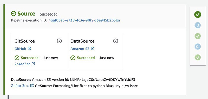
Specifically, you see a VersionId in the output from this cell:

{'ResponseMetadata': {'RequestId': 'ED389631CA6A9815',
  'HostId': '3jAk/BJoRb78yElCVxrEpekVKE34j/WKIqwTIJIxgb2IoUSV8khz7T5GLiSKO/u0c66h8/Iye9w=',
  'HTTPStatusCode': 200,
  'HTTPHeaders': {'x-amz-id-2': '3jAk/BJoRb78yElCVxrEpekVKE34j/WKIqwTIJIxgb2IoUSV8khz7T5GLiSKO/u0c66h8/Iye9w=',
   'x-amz-request-id': 'ED389631CA6A9815',
   'date': 'Mon, 15 Jun 2020 05:06:39 GMT',
   'x-amz-version-id': 'NJMR4LzjbC0cNarlnZwtDKYwTnYsIdF3',
   'etag': '"47f9ca2b44d0e2d66def2f098dd13094"',
   'content-length': '0',
   'server': 'AmazonS3'},
  'RetryAttempts': 0},
 'ETag': '"47f9ca2b44d0e2d66def2f098dd13094"',
 'VersionId': 'NJMR4LzjbC0cNarlnZwtDKYwTnYsIdF3'}

This corresponds to the Amazon S3 data source version id in the pipeline. See the following screenshot.

The Build stage in the pipeline runs a CodeBuild job defined in buildspec.yml that runs the following actions:

• Runs the model run.py Python file to output the training job definition.
• Packages CloudFormation templates for the Dev and Prod deploy stages, including the API Gateway and Lambda resources for the blue/green deployment.

The source code for the model and API are available in the Git repository. See the following directory tree:

├── api
│   ├── __init__.py
│   ├── app.py
│   ├── post_traffic_hook.py
│   └── pre_traffic_hook.py
├── model
│   ├── buildspec.yml
│   ├── requirements.txt
│   └── run.py

The Build stage is also responsible for deploying the Lambda custom resources referenced in the CloudFormation stacks.

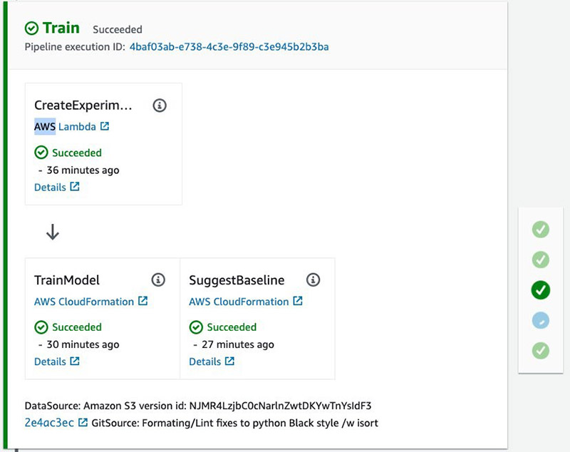
Step 3: Wait for Training Job

When the training and baseline job is complete, you can inspect the metrics associated with the Experiment and Trial component linked to the pipeline execution ID.

In addition to the train metrics, there is another job to create a baseline, which outputs statistics and constraints used for model monitoring after the model is deployed to production. The following table summarizes the parameters.

These actions run in parallel using custom AWS CloudFormation resources that poll the jobs every 2 minutes to check on their status. See the following screenshot.

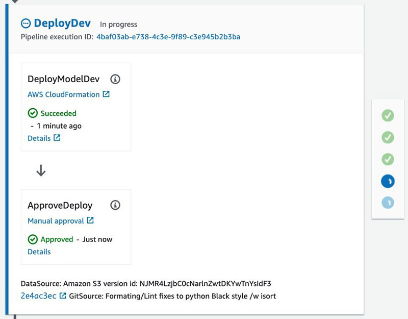
Step 4: Test Dev Deployment

With the training job complete, the development endpoint is deployed in the next stage. The notebook polls the endpoint status until it becomes InService. See the following code:

sm = boto3.client('sagemaker')

while True:
    try:
        response = sm.describe_endpoint(EndpointName=dev_endpoint_name)
        print("Endpoint status: {}".format(response['EndpointStatus']))
        if response['EndpointStatus'] == 'InService':
            break
    except:
        pass 
    time.sleep(10)

With an endpoint in service, you can use the notebook to predict the expected fare amount based on the inputs from the test dataset. See the following code:

pred_df = pd.DataFrame({'total_amount_predictions': predictions })
pred_df = test_df.join(pred_df) # Join on all
pred_df['error'] = abs(pred_df['total_amount']-pred_df['total_amount_predictions'])

ax = pred_df.tail(1000).plot.scatter(x='total_amount_predictions', y='total_amount', 
                                     c='error', title='actual amount vs pred')

You can join these predictions back to the target total amount, and visualize them in a scatter plot.

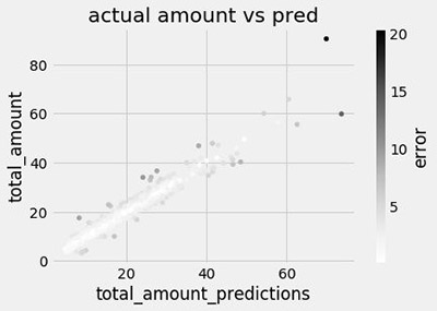
The notebook also calculates the root mean square error, which is commonly used in regression problems like this.

Step 5: Approve Prod Deployment

If you’re happy with the model, you can approve it directly using the Jupyter notebook widget.

As an administrator, you can also approve or reject the manual approval on the AWS CodePipeline console.

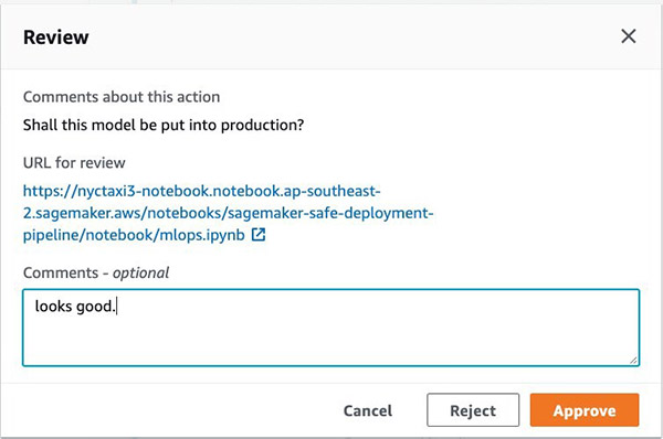
Approving this action moves the pipeline to the final blue/green production deployment stage.

Step 6: Test Prod Deployment

Production deployment is managed through a single AWS CloudFormation which performs several dependent actions, including:

1. Creates an Amazon SageMaker endpoint with AutoScaling enabled
2. Updates the endpoints to enable data capture and schedule model monitoring
3. Calls CodeDeploy to create or update a RESTful API using blue/green Lambda deployment

The following diagram illustrates this workflow.

The first time this pipeline is run, there’s no existing Blue deployment, so CodeDeploy creates a new API Gateway and Lambda resource, which is configured to invoke an Amazon SageMaker endpoint that has been configured with AutoScaling and data capture enabled.

Rerunning the build pipeline

If you go back to Step 2 in the notebook and upload a new Amazon S3 data source artifact, you trigger a new build in the pipeline, which results in an update to the production deployment CloudFormation stack. This results in a new Lambda version pointing to a second Green Amazon SageMaker endpoint being created in parallel with the original Blue endpoint.

You can use the notebook to query the most recent events in the CloudFormation stack associated with this deployment. See the following code:

from datetime import datetime
from dateutil.tz import tzlocal

def get_event_dataframe(events):
    stack_cols = [
        "LogicalResourceId",
        "ResourceStatus",
        "ResourceStatusReason",
        "Timestamp",
    ]
    stack_event_df = pd.DataFrame(events)[stack_cols].fillna("")
    stack_event_df["TimeAgo"] = datetime.now(tzlocal()) - stack_event_df["Timestamp"]
    return stack_event_df.drop("Timestamp", axis=1)

# Get latest stack events
response = cfn.describe_stack_events(StackName=stack_name)
get_event_dataframe(response["StackEvents"]).head()

The output shows the latest events and, for this post, illustrates that the endpoint has been updated for data capture and CodeDeploy is in the process of switching traffic to the new endpoint. The following table summarizes the output.

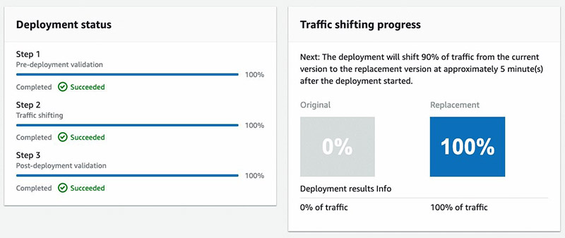
When the Blue endpoint status is InService, the notebook outputs a link to the CodeDeploy Deployment Application page, where you can watch as the traffic shifts from the original to the replacement endpoint.

A successful blue/green deployment is contingent on the post-deployment validation passing, which for this post is configured to check that live traffic has been received; evident by data capture logs in Amazon S3.

The notebook guides you through the process of sending requests to the RESTful API, which is provided as an output in the CloudFormation stack. See the following code:

from urllib import request

headers = {"Content-type": "text/csv"}
payload = test_df[test_df.columns[1:]].head(1).to_csv(header=False, index=False).encode('utf-8')

while True:
    try:
        resp = request.urlopen(request.Request(outputs['RestApi'], data=payload, headers=headers))
        print("Response code: %d: endpoint: %s" % (resp.getcode(), resp.getheader('x-sagemaker-endpoint')))
        status, outputs = get_stack_status(stack_name) 
        if status.endswith('COMPLETE'):
            print('Deployment completen')
            break
    except Exception as e:
        pass
    time.sleep(10)

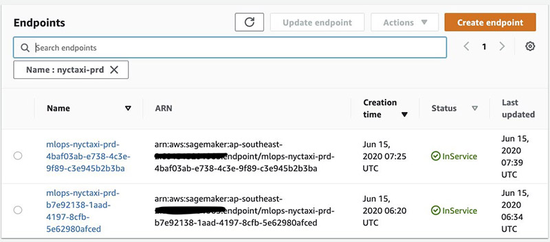
This cell loops every 10 seconds until the deployment is complete, retrieving a header that indicates which Amazon SageMaker endpoint was hit for that request. Because we’re using the canary mode, you see a small sample of hits from the new target endpoint (ending in c3e945b2b3ba) until the CodeDeploy process completes successfully, at which point the original endpoint (ending in 5e62980afced) is deleted because it’s no longer required. See the following output:

Response code: 200: endpoint: mlops-nyctaxi-prd-b7e92138-1aad-4197-8cfb-5e62980afced
Response code: 200: endpoint: mlops-nyctaxi-prd-4baf03ab-e738-4c3e-9f89-c3e945b2b3ba
Response code: 200: endpoint: mlops-nyctaxi-prd-b7e92138-1aad-4197-8cfb-5e62980afced
Response code: 200: endpoint: mlops-nyctaxi-prd-b7e92138-1aad-4197-8cfb-5e62980afced
Response code: 200: endpoint: mlops-nyctaxi-prd-b7e92138-1aad-4197-8cfb-5e62980afced
Response code: 200: endpoint: mlops-nyctaxi-prd-b7e92138-1aad-4197-8cfb-5e62980afced
Response code: 200: endpoint: mlops-nyctaxi-prd-4baf03ab-e738-4c3e-9f89-c3e945b2b3ba
Response code: 200: endpoint: mlops-nyctaxi-prd-4baf03ab-e738-4c3e-9f89-c3e945b2b3ba
Response code: 200: endpoint: mlops-nyctaxi-prd-4baf03ab-e738-4c3e-9f89-c3e945b2b3ba
Response code: 200: endpoint: mlops-nyctaxi-prd-4baf03ab-e738-4c3e-9f89-c3e945b2b3ba
Response code: 200: endpoint: mlops-nyctaxi-prd-4baf03ab-e738-4c3e-9f89-c3e945b2b3ba
Response code: 200: endpoint: mlops-nyctaxi-prd-4baf03ab-e738-4c3e-9f89-c3e945b2b3ba
Response code: 200: endpoint: mlops-nyctaxi-prd-4baf03ab-e738-4c3e-9f89-c3e945b2b3ba

Step 7: Model Monitoring

As part of the production deployment, Amazon SageMaker Model Monitor is scheduled to run every hour on the newly created endpoint, which has been configured to capture data request input and output data to Amazon S3.

You can use the notebook to list these data capture files, which are collected as a series of JSON lines. See the following code:

bucket = sagemaker_session.default_bucket()
data_capture_logs_uri = 's3://{}/{}/datacapture/{}'.format(bucket, model_name, prd_endpoint_name)

capture_files = S3Downloader.list(data_capture_logs_uri)
print('Found {} files'.format(len(capture_files)))

if capture_files:
    # Get the first line of the most recent file    
    event = json.loads(S3Downloader.read_file(capture_files[-1]).split('n')[0])
    print('nLast file:n{}'.format(json.dumps(event, indent=2)))

If you take the first line of the last file, you can see that the input contains a CSV with fields for the following:

• Duration (10.65 minutes)
• Passenger count (1 person)
• Trip distance (2.56 miles)

The output is the following:

• Predicted fare ($12.70)

See the following code:

Found 8 files

Last file:
{
  "captureData": {
    "endpointInput": {
      "observedContentType": "text/csv",
      "mode": "INPUT",
      "data": "10.65,1,2.56n",
      "encoding": "CSV"
    },
    "endpointOutput": {
      "observedContentType": "text/csv; charset=utf-8",
      "mode": "OUTPUT",
      "data": "12.720224380493164",
      "encoding": "CSV"
    }
  },
  "eventMetadata": {
    "eventId": "44daf7d7-97c8-4504-8b3d-399891f8f217",
    "inferenceTime": "2020-05-12T04:18:39Z"
  },
  "eventVersion": "0"
}

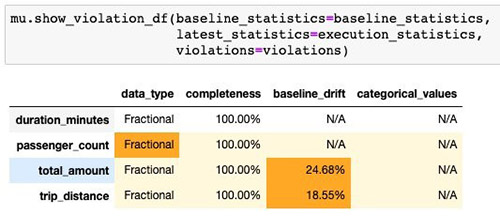
The monitoring job rolls up all the results in the last hour and compares these to the baseline statistics and constraints captured in the Train phase of the pipeline. As we can see from the notebook visualization, we can detect baseline drift with respect to the total_amount and trip_distance inputs, which were randomly sampled from our test set.

Step 8: CloudWatch Monitoring

AWS CloudWatch Synthetics provides you a way to set up a canary to test that your API is returning a successful HTTP 200 response on a regular interval. This is a great way to validate that the blue/green deployment isn’t causing any downtime for your end-users.

The notebook loads the canary.js template, which is parameterized with a rest_uri and payload invoked from the Lambda layer created by the canary, which is configured to hit the production REST API every 10 minutes. See the following code:

from urllib.parse import urlparse
from string import Template
from io import BytesIO
import zipfile
import sagemaker

# Format the canary_js with rest_api and payload
rest_url = urlparse(rest_api)
with open('canary.js') as f:
    canary_js = Template(f.read()).substitute(hostname=rest_url.netloc, 
                                              path=rest_url.path, 
                                              data=payload.decode('utf-8').strip())
# Write the zip file
zip_buffer = BytesIO()
with zipfile.ZipFile(zip_buffer, 'w') as zf:
    zip_path = 'nodejs/node_modules/apiCanaryBlueprint.js' # Set a valid path
    zip_info = zipfile.ZipInfo(zip_path)
    zip_info.external_attr = 0o0755 << 16 # Ensure the file is readable
    zf.writestr(zip_info, canary_js)
zip_buffer.seek(0)

# Create the canary
synth = boto3.client('synthetics')

role = sagemaker.get_execution_role()
s3_canary_uri = 's3://{}/{}'.format(artifact_bucket, model_name)
canary_name = 'mlops-{}'.format(model_name)

response = synth.create_canary(
    Name=canary_name,
    Code={
        'ZipFile': bytearray(zip_buffer.read()),
        'Handler': 'apiCanaryBlueprint.handler'
    },
    ArtifactS3Location=s3_canary_uri,
    ExecutionRoleArn=role,
    Schedule={ 
        'Expression': 'rate(10 minutes)', 
        'DurationInSeconds': 0 },
    RunConfig={
        'TimeoutInSeconds': 60,
        'MemoryInMB': 960
    },
    SuccessRetentionPeriodInDays=31,
    FailureRetentionPeriodInDays=31,
    RuntimeVersion='syn-1.0',
)

You can also configure an alarm for this canary to alert when the success rates drop below 90%:

cloudwatch = boto3.client('cloudwatch')

canary_alarm_name = '{}-synth-lt-threshold'.format(canary_name)

response = cloudwatch.put_metric_alarm(
    AlarmName=canary_alarm_name,
    ComparisonOperator='LessThanThreshold',
    EvaluationPeriods=1,
    DatapointsToAlarm=1,
    Period=600, # 10 minute interval
    Statistic='Average',
    Threshold=90.0,
    ActionsEnabled=False,
    AlarmDescription='SuccessPercent LessThanThreshold 90%',
    Namespace='CloudWatchSynthetics',
    MetricName='SuccessPercent',
    Dimensions=[
        {
          'Name': 'CanaryName',
          'Value': canary_name
        },
    ],
    Unit='Seconds'
)

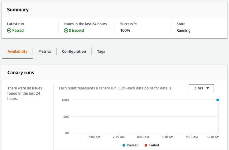
With the canary created, you can choose the link provided to view the detail on the AWS CloudWatch console, which includes metrics such as uptime and as the logs output from your Lambda code.

Returning to the notebook, create a CloudWatch dashboard from a template parametrized with the current region, account_id and model_name:

sts = boto3.client('sts')
account_id = sts.get_caller_identity().get('Account')
dashboard_name = 'mlops-{}'.format(model_name)

with open('dashboard.json') as f:
    dashboard_body = Template(f.read()).substitute(region=region, 
                                                   account_id=account_id, 
                                                   model_name=model_name)
    response = cloudwatch.put_dashboard(
        DashboardName=dashboard_name,
        DashboardBody=dashboard_body
    )

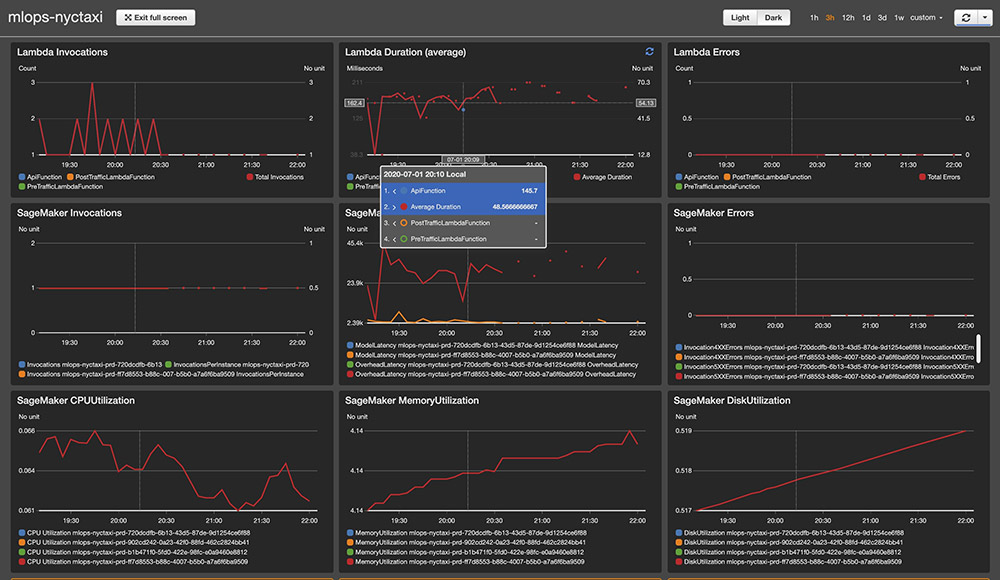
This creates a dashboard with a four-row-by-three-column layout with metrics for your production deployment, including the following:

• Lambda metrics for latency and throughput
• Amazon SageMaker endpoint
• CloudWatch alarms for CodeDeploy and model drift

You can choose the link to open the dashboard in full screen and use Dark mode. See the following screenshot.

Cleaning up

You can remove the canary and CloudWatch dashboard directly within the notebook. The pipeline created Amazon SageMaker training, baseline jobs, and endpoints using AWS CloudFormation, so to clean up these resources, delete the stacks prefixed with the name of your model. For example, for nyctaxi, the resources are the following:

• nyctaxi-devploy-prd
• nyctaxi-devploy-dev
• nyctaxi-training-job
• nyctaxi-suggest-baseline

After these are deleted, complete your cleanup by emptying the S3 bucket created to store your pipeline artefacts, and delete the original stack, which removes the pipeline, Amazon SageMaker notebook, and other resources.

Conclusion

In this post, we walked through creating an end-to-end safe deployment pipeline for Amazon SageMaker models using native AWS development tools CodePipeline, CodeBuild, and CodeDeploy. We demonstrated how you can trigger the pipeline directly from within an Amazon SageMaker notebook, validate and approve deployment to production, and continue to monitor your models after they go live. By running the pipeline a second time, we saw how CodeDeploy created a new Green replacement endpoint that was cut over to after the post-deployment validated it had received live traffic. Finally, we saw how to use CloudWatch Synthetics to constantly monitor our live endpoints and visualize metrics in a custom CloudWatch dashboard.

You could easily extend this solution to support your own dataset and model. The source code is available on the GitHub repo.

About the Author

Julian Bright is an Sr. AI/ML Specialist Solutions Architect based out of Melbourne, Australia. Julian works as part of the global AWS machine learning team and is passionate about helping customers realise their AI and ML journey through MLOps. In his spare time he loves running around after his kids, playing soccer and getting outdoors.

Read More

The machine learning (ML) model-building process requires data scientists to manually prepare data features, select an appropriate algorithm, and optimize its model parameters. It involves a lot of effort and expertise. Amazon SageMaker Autopilot removes the heavy lifting required by this ML process. It inspects your dataset, generates several ML pipelines, and compares their performance to produce a leaderboard of candidate pipelines. Each candidate pipeline is a combination of data preprocessing steps, an ML algorithm, and its optimized hyperparameters. You can easily deploy any of these candidate pipelines to use for real-time prediction or batch prediction.

But what if you want to preprocess the data before invoking Amazon SageMaker Autopilot? For example, you might have a dataset with several features and need customized feature selection to remove irrelevant variables before using it to train a model in an Autopilot job. Then you need to incorporate your custom processing code into the pipeline when deploying it to a real-time endpoint or for batch processing. This post shows you how to customize an Autopilot inference pipeline with your own data processing code. The code from this post is available in the GitHub repo.

Solution overview

The solution of customizing a pipeline that combines custom feature selection with Autopilot models includes the following steps:

1. Prepare a dataset with 100 features as the example dataset for this post and upload it to Amazon Simple Storage Service (Amazon S3).
2. Train the feature selection model and prepare the dataset using sagemaker-scikit-learn-container to feed to Autopilot.
3. Configure and launch the Autopilot job.
4. Create an inference pipeline that combines feature selection with the Autopilot models.
5. Make predictions with the inference pipeline.

The following diagram outlines the architecture of this workflow.

Preparing and uploading the dataset

First, we generate a regression dataset using sklearn.datasets.make_regression. Set the number of features to 100. Five of these features are informative. The 100 variable names are indexed as x_i and the name of the target variable is y:

X, y = make_regression(n_features = 100, n_samples = 1500, n_informative = 5, random_state=0)
df_X = pd.DataFrame(X).rename(columns=lambda x: 'x_'+ str(x))
df_y = pd.DataFrame(y).rename(columns=lambda x: 'y')
df = pd.concat([df_X, df_y], axis=1)

The following screenshot shows the data generated. You upload this dataset to Amazon S3 to use in later steps.

Training the feature selection model and preparing the dataset

Feature selection is the process of selecting a subset of the most relevant features on which to train an ML model. This simplification shortens training time and reduces the chance of overfitting. The sklearn.feature_selection module contains several feature selection algorithms. For this post, we use the following:

• feature_selection.RFE – The recursive feature elimination (RFE) algorithm selects features by recursively considering smaller and smaller sets of features. First, the estimator is trained on the initial set of features and the importance of each feature is obtained. Then, the least important features are pruned from the current set of features. We use Epsilon-Support Vector Regression (sklearn.svm.SVR) as our learning estimator for RFE.
• feature_selection.SelectKBest – The SelectKBest algorithm selects the k features that have the highest scores of a specified metric. We use mutual information and f regression as the score functions—both methods measure the dependency between variables. For more information about f regression and mutual information, see Feature Selection.

We stack these three feature selection algorithms into one sklearn.pipeline.Pipeline. RFE by default eliminates 50% of the total features. We use SelectKBest to select the top 30 features using the f_regression method and reduce the number of features to 10 using the mutual_info_regression method. Note that the feature selection algorithms used here are for demonstration purposes only. You can update the script to incorporate feature selection algorithm of your choice.

We also create a Python script for feature selection. In the following code example, we build a sklearn Pipeline object that implements the method we described:

'''Feature selection pipeline'''
feature_selection_pipe = pipe = Pipeline([
                 ('svr', RFE(SVR(kernel="linear"))),
                 ('f_reg',SelectKBest(f_regression, k=30)),
                ('mut_info',SelectKBest(mutual_info_regression, k=10))
                ])
feature_selection_pipe.fit(X_train,y_train)

To provide visibility on which features are selected, we use the following script to generate and save the names of selected features as a list:

  '''Save selected feature names'''
    feature_names = concat_data.columns[:-1]
    feature_names = feature_names[pipe.named_steps['svr'].get_support()]
    feature_names = feature_names[pipe.named_steps['f_reg'].get_support()]
    feature_names = feature_names[pipe.named_steps['mut_info'].get_support()]

We use the Amazon SageMaker SKLearn Estimator with a feature selection script as an entry point. The script is very similar to a training script you might run outside of Amazon SageMaker, but you can access useful properties about the training environment through various environment variables, such as SM_MODEL_DIR, which represents the path to the directory inside the container to write model artifacts to. These artifacts are uploaded to the Amazon S3 output path by the Amazon SageMaker training job. After training is complete, we save model artifacts and selected column names for use during inference to SM_MODEL_DIR. See the following code:

    joblib.dump(feature_selection_pipe, os.path.join(args.model_dir, "model.joblib"))
    ...
    joblib.dump(feature_selection_pipe, os.path.join(args.model_dir, "selected_feature_names.joblib"))

Although we use feature selection algorithms in this post, you can customize and add additional data preprocessing code, such as code for data imputation or other forms of data cleaning, to this entry point script.

Now that our feature selection model is properly fitted, we transform the raw input data to the training dataset with selected features. To use Amazon SageMaker batch transform to directly process the raw data and store back to Amazon S3, enter the following code:

# Define a SKLearn Transformer from the trained SKLearn Estimator
transformer_output = os.path.join('s3://',bucket, prefix, 'Feature_selection_output/')
transformer = sklearn_preprocessor.transformer(
    instance_count=1, 
    instance_type='ml.m4.xlarge',
    output_path = transformer_output,
    assemble_with = 'Line',
    accept = 'text/csv')
    
transformer.transform(train_input, content_type='text/csv') 

The notebook contains an additional step that adds the selected column names as headers to the generated CSV data files.

Configuring and launching the Autopilot job

The output from batch transform is the new training dataset for Autopilot. The new dataset has 10 features. To use Autopilot, we simply provide our new dataset and choose the target column to be y. Autopilot automatically inspects our dataset and runs several candidates to determine the optimal combination of data preprocessing steps, ML algorithms, and hyperparameters. Before launching the Autopilot job, we define the job input configuration, output configuration, and stopping criteria:

input_data_config = [{
      'DataSource': {
        'S3DataSource': {
          'S3DataType': 'S3Prefix',
          'S3Uri': 's3://{}/{}/training_data_new'.format(bucket,prefix)
        }
      },
      'TargetAttributeName': 'y'
    }
  ]

output_data_config = {
    'S3OutputPath': 's3://{}/{}/autopilot_job_output'.format(bucket,prefix)
  }

AutoML_Job_Config = {
    'CompletionCriteria': {
            'MaxCandidates': 50,
            'MaxAutoMLJobRuntimeInSeconds': 1800
        }
  }

Then we call the create_auto_ml_job API to launch the Autopilot job:

sm = boto3.Session().client(service_name='sagemaker',region_name=region)
timestamp_suffix = strftime('%d-%H-%M-%S', gmtime())

auto_ml_job_name = 'automl-blog' + timestamp_suffix
print('AutoMLJobName: ' + auto_ml_job_name)

sm.create_auto_ml_job(AutoMLJobName=auto_ml_job_name,
                      InputDataConfig=input_data_config,
                      OutputDataConfig=output_data_config,
                      AutoMLJobConfig = AutoML_Job_Config,
                      RoleArn=role)

Creating an inference pipeline that combines feature selection with Autopilot models

So far, we have created a model that takes raw data with 100 features and selects the 10 most relevant features. We also used Autopilot to create data processing and ML models to predict y. We now combine the feature selection model with Autopilot models to create an inference pipeline. After defining the models and assigning names, we create a PipelineModel that points to our preprocessing and prediction models. The pipeline.py file is available on GitHub. See the following code:

sklearn_image = sklearn_preprocessor.image_name
container_1_source = os.path.join("s3://", 
                                  sagemaker_session.default_bucket(), 
                                  sklearn_preprocessor.latest_training_job.job_name,
                                  "sourcedir.tar.gz"
                                 )
inference_containers = [
        {
            'Image': sklearn_image,
            'ModelDataUrl': sklearn_preprocessor.model_data,
            'Environment': {
                'SAGEMAKER_SUBMIT_DIRECTORY':container_1_source,
                'SAGEMAKER_DEFAULT_INVOCATIONS_ACCEPT': "text/csv",
                'SAGEMAKER_PROGRAM':'sklearn_feature_selection.py'
            }
        }]

inference_containers.extend(best_candidate['InferenceContainers'])

response = sagemaker.create_model(
        ModelName=pipeline_name,
        Containers=inference_containers,
        ExecutionRoleArn=role)

We then deploy the pipeline model to a single endpoint:

response = sagemaker.create_endpoint(
        EndpointName=pipeline_endpoint_name,
        EndpointConfigName=pipeline_endpoint_config_name,
    )

Making predictions with the inference pipeline

We can test our pipeline by sending data for prediction. The pipeline accepts raw data, transforms it using the feature selection model, and creates a prediction using the models Autopilot generated.

First, we define a payload variable that contains the data we want to send through the pipeline. We use the first five rows of the training data as our payload. Then we define a predictor using our pipeline endpoint, send the payload to the predictor, and print the model prediction:

from sagemaker.predictor import RealTimePredictor, csv_serializer
from sagemaker.content_types import CONTENT_TYPE_CSV
predictor = RealTimePredictor(
    endpoint=pipeline_endpoint_name,
    serializer=csv_serializer,
    sagemaker_session=sagemaker_session,
    content_type=CONTENT_TYPE_CSV,
    accept=CONTENT_TYPE_CSV)

predictor.content_type = 'text/csv'
predictor.predict(test_data.to_csv(sep=',', header=True, index=False)).decode('utf-8')

Our Amazon SageMaker endpoint returns one prediction for each corresponding row of the data sent. See the following code:

'-102.248855591n-165.823532104n115.50453186n111.306632996n5.91651535034'

Deleting the endpoint

When we are finished with the endpoint, we delete it to save cost:

sm_client = sagemaker_session.boto_session.client('sagemaker')
sm_client.delete_endpoint(EndpointName=pipeline_endpoint_name)

Conclusions

In this post, we demonstrated how to customize an Autopilot inference pipeline with your own data processing code. We first trained a feature selection model and converted our raw data using the trained feature selection model. Then we launched an Amazon SageMaker Autopilot job that automatically trained and tuned the best ML models for our regression problem. We also built an inference pipeline that combined feature selection with the Autopilot models. Lastly, we made predictions with the inference pipeline. For more about Amazon SageMaker Pilot, please see Amazon SageMaker Autopilot.

About the Authors

Qingwei Li is a Machine Learning Specialist at Amazon Web Services. He received his Ph.D. in Operations Research after he broke his advisor’s research grant account and failed to deliver the Nobel Prize he promised. Currently he helps customers in financial service and insurance industry build machine learning solutions on AWS. In his spare time, he likes reading and teaching.

Piali Das is a Senior Software Engineer in the AWS SageMaker Autopilot team. She previously contributed to building SageMaker Algorithms. She enjoys scientific programming in general and has developed an interest in machine learning and distributed systems.

Read More

There are many techniques to train deep learning models with a small amount of data. Examples include transfer learning, few-shot learning, or even one-shot learning for an image classification task and fine-tuning for language models based on a pre-trained BERT or GPT2 model. However, you may still have a use case in which you need a large amount of training data. For instance, if the images are quite different from ImageNet or your language corpus is domain specific rather than general, then it’s hard to achieve the desired model performance with transfer learning. If you are deep learning researchers, you want to try new ideas or approaches from scratch. In these cases, your task is to train a large deep learning model with a large dataset, which can take days, weeks, or even months if you don’t use the proper methods for training large-scale models.

In this post, I explain how to run multi-GPU training on a single instance on Amazon SageMaker, and discuss efficient multi-GPU and multi-node distributed training on Amazon SageMaker.

Basics on Horovod

When you train a model with a large amount of data, you should distribute the training across multiple GPUs on either a single instance or multiple instances. Deep learning frameworks provide their own methods to support multi-GPU training or distributed training. However, there is another way to accomplish this using distributed deep learning framework such as Horovod. Horovod is Uber’s open-source framework for distributed deep learning, and it’s available for use with most popular deep learning toolkits like TensorFlow, Keras, PyTorch, and Apache MXNet. It uses the all-reduce algorithm for fast distributed training rather than using a parameter server approach, and includes multiple optimization methods to make distributed training faster. For more information, see Meet Horovod: Uber’s Open Source Distributed Deep Learning Framework for TensorFlow.

Preparing your data for Horovod

When you start a training job using Horovod, Horovod launches an independent process for each worker per one GPU in the Horovod cluster. For example, four worker processes start when you run a Horovod training job with one training instance with four GPUs (one Amazon SageMaker ml.p3.8xlarge or Amazon Elastic Compute Cloud (Amazon EC2) p3.8xlarge instance). All four Horovod workers read their own dataset, which is already split into shards as data parallelism. If there are 40,000 training samples, each worker gets 10,000 training samples without duplication. If you use Horovod for distributed training or even multi-GPU training, you should do this data shard preparation beforehand and let the worker read its shard from the file system. (There are deep learning frameworks that do this automatically on the fly, such as PyTorch’s DataParallel and DistributedDataParallel.)

The following diagram illustrates two architectures for storing shards.

You can provide a dataset for an Amazon SageMaker training job in several different ways. One typical method is to store all your dataset in your Amazon Simple Storage Service (Amazon S3) bucket and access them when needed. Although you may use a shared file system like Amazon FSx for Lustre or Amazon Elastic File System (Amazon EFS) for data storage, you can also avoid the additional cost by retrieving data directly from Amazon S3 via two input modes available to Amazon SageMaker: File mode and Pipe mode.

In File mode, when the training job is launched in Amazon SageMaker, the defined dataset is transferred from the specified S3 bucket to training instances, and they are placed in a directory under a certain directory. However, if the dataset is huge, it takes a long time to copy objects from the bucket to the training instances’ storage, and the start of training is delayed until the data transfer is complete. In some cases, this might slow down the machine learning (ML) pipeline, and even slow down innovation or research speed.

You can also access the dataset stored in Amazon S3 directly through Pipe mode. Pipe mode creates a direct input pipe between the training instance and S3 bucket, and allows the training process to access the objects directly without copying it all into training instances before training begins. To access a dataset in a given Amazon S3 URI as Pipe mode, you set the input mode to Pipe when you create an Amazon SageMaker estimator. See the following code:

from sagemaker.tensorflow import TensorFlow

tf_estimator = TensorFlow(entry_point='train.py',
                          role='SageMakerRole',
                          train_instance_type='ml.p3.2xlarge',
                          train_instance_count=2,
                          framework_version='2.1.0',
                          py_version='py3',
                          input_mode='Pipe')

With Pipe mode, the training data is available as a FIFO stream. There is an extension of a TensorFlow dataset that makes it easy to access a streamed dataset. For more information about Pipe mode and TensorFlow, see Accelerate model training using faster Pipe mode on Amazon SageMaker and the Amazon SageMaker TensorFlow extension GitHub repo.

Pipe mode with Horovod

There is a special care needed when you use Horovod with Pipe mode for either multi-GPU training using a single training instance or distributed training using multiple training instances with multiple GPU cores. The following diagram illustrates this architecture.

Pipe mode streams data from Amazon S3 into Unix Named Pipes or FIFOs in the training instances. A FIFO file supports only a single writer/reader pair, and there is one FIFO created for one channel per epoch. Normally, people define one channel for the training dataset and another for the validation or test dataset and pass these input channels to the training job as parameters of Amazon SageMaker estimator’s fit() function. See the following code:

from sagemaker.session import s3_input

input_channel = {'train': s3_input('s3://your-bucket-name/train-dataset/')}

tf_estimator.fit(inputs=input_channel)     

What does this mean in Horovod multi-GPU training? Processes launched by a multi-GPU training job using Horovod compete each other on a single FIFO, which can’t be accessed simultaneously by multiple processes. Because only one worker process can access the FIFO concurrently and it doesn’t release the handle until the training job is finished, all the other workers can’t read data from the same FIFO and therefore the training falls into a deadlock-style infinite loop. If you see repeated messages similar to the following code, this is the problem you are encountering:

[1,0]<stderr>:Stalled ranks:
[1,0]<stderr>:0: [training/Adam/DistributedAdam_Allreduce/HorovodAllreduce_training_Adam_gradients_AddN_11_0, training/Adam/DistributedAdam_Allreduce/HorovodAllreduce_training_Adam_gradients_AddN_12_0, training/Adam/DistributedAdam_Allreduce/HorovodAllreduce_training_Adam_gradients_AddN_14_0, training/Adam/DistributedAdam_Allreduce/HorovodAllreduce_training_Adam_gradients_AddN_15_0, training/Adam/DistributedAdam_Allreduce/HorovodAllreduce_training_Adam_gradients_AddN_18_0, training/Adam/DistributedAdam_Allreduce/HorovodAllreduce_training_Adam_gradients_AddN_19_0 ...]
[1,0]<stderr>:2: [training/Adam/DistributedAdam_Allreduce/HorovodAllreduce_training_Adam_gradients_AddN_11_0, training/Adam/DistributedAdam_Allreduce/HorovodAllreduce_training_Adam_gradients_AddN_12_0, training/Adam/DistributedAdam_Allreduce/HorovodAllreduce_training_Adam_gradients_AddN_14_0, training/Adam/DistributedAdam_Allreduce/HorovodAllreduce_training_Adam_gradients_AddN_15_0, training/Adam/DistributedAdam_Allreduce/HorovodAllreduce_training_Adam_gradients_AddN_18_0, training/Adam/DistributedAdam_Allreduce/HorovodAllreduce_training_Adam_gradients_AddN_19_0 ...]
[1,0]<stderr>:3: [training/Adam/DistributedAdam_Allreduce/HorovodAllreduce_training_Adam_gradients_AddN_11_0, training/Adam/DistributedAdam_Allreduce/HorovodAllreduce_training_Adam_gradients_AddN_12_0, training/Adam/DistributedAdam_Allreduce/HorovodAllreduce_training_Adam_gradients_AddN_14_0, training/Adam/DistributedAdam_Allreduce/HorovodAllreduce_training_Adam_gradients_AddN_15_0, training/Adam/DistributedAdam_Allreduce/HorovodAllreduce_training_Adam_gradients_AddN_18_0, training/Adam/DistributedAdam_Allreduce/HorovodAllreduce_training_Adam_gradients_AddN_19_0 ...]

You should shard the dataset in an S3 bucket into the number of GPUs to be used for training. If you have 4,000 TensorFlow record files, and you train a model using one ml.p3.8xlarge with four GPUs, you can place each 1,000 TensorFlow record files under a different prefix, as in the following code:

s3://your-bucket-name/train/0/
s3://your-bucket-name/train/1/
s3://your-bucket-name/train/2/
s3://your-bucket-name/train/3/

Sharding a dataset using SharedByS3Key as an Amazon S3 data distribution type isn’t applicable to Horovod. This is because with SharedByS3Key, the shard is done per instance, not per worker, and there are as many workers as GPUs in an instance. Also, the input channel is still one per instance. Therefore, you need to shard the data to have as many shards as the total number of GPU cores in the Horovod cluster.

You then define four input channels for Amazon SageMaker training. See the following code:

from sagemaker.session import s3_input

shuffle_config = sagemaker.session.ShuffleConfig(234)

train_s3_uri_prefix = 's3://your-bucket-name/train'
input_channels = {}

for idx in range(4):
    train_s3_uri = f'{train_s3_uri_prefix}/train/{idx}/'
    train_s3_input = s3_input(train_s3_uri, shuffle_config=shuffle_config)
    input_channels[f'train_{idx}'] = train_s3_input

ShuffleConfig makes sure that the order of the files under the Amazon S3 prefix is randomized for every epoch. For more information, see ShuffleConfig.

Use the following channel definition when you call the fit method on the Amazon SageMaker estimator:

tf_estimator.fit(input_channels)

For validation and test tasks, you only run these tasks on a single worker (normally on the primary worker or a worker of Rank 0). You don’t need to have multiple validation or test channels. However, if you use the tf.keras.model.fit() function for training, the training gets stalled if only one Horovod worker does validation (for more information, see issue #600 on the Horovod GitHub repo). If validation is needed with tf.keras.model.fit(), you also have to provide each input channel for the validation dataset to each worker just like the training input channel. Keep in mind that as of July 2020, the total number of Pipe input channels is limited to 20 for a training job. See the following code:

validation_s3_uri = 's3://your-bucket-name/validation/'

for idx in range(4):
    validation_s3_input = s3_input(validation_s3_uri)
    input_channels[f'validation_{idx}'] = validation_s3_input
    
eval_s3_uri = 's3://your-bucket-name/eval/'
eval_s3_input = s3_input(eval_s3_uri)
input_channels['eval'] = eval_s3_input

Instead of using the prefix of the S3 bucket, you can use a plain ManifestFile that contains a list of object keys. For more information, see Input Data.

Using the data channel in training code

In the training script, you need to force each Horovod worker process to access its own shard so two workers don’t access the same input channel. In our use case, the names of input channels are defined using indexes starting from 0, so you can use the hvd.rank() function, which gives the cluster-wide unique rank index of the current worker process, and the rank also begins from 0 (see line 13 in the following code). For this post, we use the Amazon SageMaker TensorFlow extension PipeModeDataset. For other deep learning frameworks, read data from a FIFO named /opt/ml/input/data/[channel_name]_${epoch} for each epoch. For more examples, see the GitHub repo.

 1: from sagemaker_tensorflow import PipeModeDataset
 2: 
 3: features = {'data': tf.FixedLenFeature([], tf.string),
 4:             'labels': tf.FixedLenFeature([], tf.int64)}
 5:
 6: def parse(record):
 7:     parsed = tf.parse_single_example(record, features)
 8:     return ({
 9:         'data': tf.decode_raw(parsed['data'], tf.float64)
10:    }, parsed['labels'])
11:
12: # For Horovod and Pipe mode, use the input channel allocated to this worker using rank information
13: channel_name = 'train_{}'.format(hvd.rank())
14:
15: ds = PipeModeDataset(channel=channel_name, record_format='TFRecord')
16: ds = ds.map(parse)
17: ds = ds.batch(64)
18: ds = ds.prefetch(10)

In a Horovod cluster with one or more instances, ranks are uniquely assigned from 0 to the number of total GPUs – 1. You don’t need to worry about the order of instances or rank number as long as you correctly defined the input channel name using indexes from 0.

Monitoring with Tensorboard

For flexible monitoring of the training process, we can invoke Tensorboard from any remote compute instance by first uploading the logs at the end of each epoch to the S3 bucket. To do so, create a callback to push the local log to an S3 bucket path that’s restricted to the primary (rank 0) compute node running on Horovod. See the following code:

class Sync2S3(tf.keras.callbacks.Callback):
    def __init__(self, logdir, s3logdir):
        super(Sync2S3, self).__init__()
        self.logdir = logdir
        self.s3logdir = s3logdir
    
    def on_epoch_end(self, batch, logs={}):
        os.system('aws s3 sync '+self.logdir+' '+self.s3logdir)

...

if hvd.rank() == 0:
    logdir = args.output_data_dir + '/' + datetime.now().strftime("%Y%m%d-%H%M%S")
    callbacks.append(TensorBoard(log_dir=logdir))
    callbacks.append(Sync2S3(logdir=logdir, s3logdir=tensorboard_logs))

With the training logs dumped in the S3 bucket, you can run Tensorboard from any server you like, including an EC2 instance, an Amazon SageMaker notebook instance, or even your local machine, as long as the server hosting Tensorboard has permissions to access the Amazon S3 log object. To launch Tensorboard, run the following shell commands in your terminal. To support direct ingestion of log data from the Amazon S3 source, Tensorboard must be running at or above version 1.14.0. The following command lines use logs located in the S3 bucket in us-east-1:

S3_REGION=us-east-1
tensorboard --logdir s3://{bucket_name}/tensorboard_logs/

If you run the preceding commands in an Amazon SageMaker notebook instance, you can access the running Tensorboard UI at https://<SageMaker-notebook-instance-name>.notebook.<notebook-region>.sagemaker.aws/proxy/6006/.

Cleaning up

After you have explored the distributed training covered in this post, clean up resources that you’re no longer using to avoid additional costs, such as the S3 buckets, FSx for Lustre, and any Amazon SageMaker instances.

Conclusion

Horovod multi-GPU or distributed training on Amazon SageMaker with Pipe mode can perform large-scale training by creating separate training channels for each shard and accessing its own shard in the data pipeline. This benefits training on Amazon SageMaker with a large training dataset by reducing the amount of time to transfer the dataset to the training instances before actual training begins.

For the complete training example to run on Amazon SageMaker, where Pipe mode and Horovod are applied together, see the GitHub repo.

About the Authors

Muhyun Kim is a data scientist at Amazon Machine Learning Solutions Lab. He solves customer’s various business problems by applying machine learning and deep learning, and also helps them gets skilled.

Jiyang Kang is a deep learning architect at Amazon Machine Learning Solutions Lab. With experience designing global enterprise workloads on AWS, he is responsible for designing and implementing ML solutions for customers’ new business problems.

Hussain Karimi is a data scientist at the Maching Learning Solutions Lab where he works with customers across various verticals to initate and build automated, algorithmic models that generate business value.

Read More

Machine learning (ML) workflows orchestrate and automate sequences of ML tasks, including data collection, training, testing, evaluating an ML model, and deploying the models for inference. AWS Step Functions automates and orchestrates Amazon SageMaker-related tasks in an end-to-end workflow. The AWS Step Functions Data Science Software Development Kit (SDK) is an open-source library that allows you to easily create workflows that preprocess data and then train and publish ML models using Amazon SageMaker and Step Functions. You can create ML workflows in Python that orchestrate AWS infrastructure at scale, without having to provision and integrate AWS services separately.

Amazon SageMaker is a fully managed service that provides every developer and data scientist with the ability to build, train, and deploy ML models at scale.

At re:Invent 2019, we announced the launch of Amazon SageMaker Processing, a new capability of Amazon SageMaker that lets you easily run your preprocessing, postprocessing, and model evaluation workloads on fully managed infrastructure.

Today, we’re happy to announce the availability of the Step Functions service integration with Amazon SageMaker Processing. This integration allows data scientists to easily integrate Amazon SageMaker Processing into their ML workflows using the Step Functions and Step Functions Data Science SDK.

Benefits of the AWS Step Functions Data Science SDK

The AWS Step Functions Data Science SDK allows data scientists to easily construct ML workflows without dealing with DevOps tasks like provisioning hardware or deploying software. The Step Functions Data Science SDK has built-in integrations with Amazon SageMaker to orchestrate ML workflows, including training, hyperparameter tuning, or deploying a model. The SDK allows you to develop and test your ML workflows locally, and provides consistency when deploying workflows to a testing or production environments on AWS.

It also includes the following benefits:

• Ease of use – You can build and orchestrate ML workflows using Python. The SDK also allows you to create reusable workflow templates that other team members can use. Step Functions allows you to easily introduce error handling, retry logic, parallel steps, and branching into the workflows. You can also build complex ML workflows using other AWS services, including native integration with the Amazon DynamoDB. Amazon SNS, Amazon SQS, Amazon EMR, AWS Lambda, AWS Glue, AWS Batch, and Amazon Elastic Container Service (Amazon ECS) – For more information, see AWS Step Functions Data Science SDK
• Agility – Step Functions allows you to build serverless workflows without needing to set up any underlying infrastructure. You can quickly build new workflows in a matter of minutes. In addition, Step Functions scales out effortlessly to match your use case.
• Cost – With Step Functions, you pay for each transition from one state to the next. Billing is metered by state transition, and you don’t pay for idle time. This keeps Step Functions cost-effective as you scale from a few runs to tens of millions. Furthermore, the native integration of the SDK with other AWS services, including Amazon SageMaker, allows you to reduce the state transitions even further. We go into more detail about one of the native integrations later in this post.

The Amazon SageMaker ProcessingStep is now available as part of the AWS Step Functions Data Science SDK. This service integration allows you to get rid of additional steps including AWS Lambda steps for creating, polling, and checking the status of Amazon SageMaker Processing jobs. You can create processing jobs by using the newly available ProcessingStep.

Prior to this launch, integrating Amazon SageMaker Processing into a Step Functions workflow required authoring AWS Lambda functions to invoke the Amazon SageMaker Processing APIs. The function used a low-level AWS SDK to construct the request parameters, call the Lambda Amazon SageMaker Processing job APIs (create_processing_job(), describe_processing_job(), list_processing_jobs(), or stop_processing_job()), and read the response objects returned. In addition, the ML engineer had to embed additional logic to check the processing job’s status using busy polling at regular intervals using additional workflow steps, including a Wait state, Choice state, and Task states to create a processing job and check the job status. The following diagram illustrates the Step Functions workflow prior to this launch

AWS Step Functions Workflow prior to the launch of “ProcessingStep”

This approach requires busy polling the processing job’s status and requires additional complexity in terms of additional steps in the overall workflow. This polling mechanism also incurs an additional cost because of the state transitions for checking the status.

New Amazon SageMaker Processing step

With new ProcessingStep, you can now choose to get the response synchronously without having to write any additional steps in the workflow.

The new ProcessingStep creates a Task state to fun the processing job. You can walk through a Step Functions Amazon SageMaker Jupyter Notebook to see how it works.

In the notebook, we create an SKLearn Amazon SageMaker Processor object. See the following code:

sklearn_processor = SKLearnProcessor(
    framework_version="0.20.0",
    role=role,
    instance_type="ml.m5.xlarge",
    instance_count=1,
    max_runtime_in_seconds=1200,
)

We then create a ProcessingStep using this processor:

processing_step = ProcessingStep(
    "SageMaker pre-processing step",
    processor=sklearn_processor,
    job_name=execution_input["PreprocessingJobName"],
    inputs=inputs,
    outputs=outputs,
    container_arguments=["--train-test-split-ratio", "0.2"],
    container_entrypoint=["python3", "/opt/ml/processing/input/code/preprocessing.py"],
)

This processing step uses the preprocessing script preprocessor.py with the argument defining the train and test dataset split ratio (for example, 0.2). For more information about input arguments, see ProcessingStep.

The new ProcessingStep launches a processing job and by default waits synchronously for it to complete. This allows you to get the status and output of the processing job in a single step as compared to writing additional steps to poll for the processing job’s status by writing a new Lambda function. The wait_for_completion parameter of the ProcessingStep is set to True to indicate that the Task state should wait for the processing job to complete before proceeding to the next step. When the ProcessingStep is finished, Step Functions makes the response of DescribeProcessingJob available as the output of the step. Step Functions internally listens to Amazon EventBridge Amazon SageMaker events to get the notifications of the processing job’s status change. This approach takes away all the heavy lifting from the end-user that would otherwise be needed in polling the job’s status.

If you need any of the values from the output of the ProcessingStep to be available to the next state in your Step Functions workflow, you can do so using the already available Choice Rules for the Choice state. See the following code:

my_choice_state.add_choice(

rule=ChoiceRule.StringEquals(variable=processing_step.output()["ProcessingJobStatus"], value="Completed")
next_step=happy_path

)

The preceding code retrieves the processing job’s status, checks if it’s in the Completed status, and sets the next state after ProcessingStep finishes.

You can further add error-handling logic in the ProcessingStep by creating a Step Functions Catch block and adding that to the list of catchers for the state by using add_catch(). See the following code:

catch_state_processing = stepfunctions.steps.states.Catch(
    error_equals=['States.TaskFailed'],
    next_step=failed_state_sagemaker_processing_failure

)
processing_step.add_catch(catch_state_processing)

The following ML workflow shows the use of ProcessingStep to preprocess a dataset prior to running a TrainingStep.

AWS Step Functions Workflow using the new “ProcessingStep”

You can also create more additional ML workflows that launch multiple parallel tasks using dynamic parallelism support in Step Functions. For example, prior to training, your workflow may run multiple independent tasks, such as anomaly detection or feature selection. You can implement these tasks by using multiple processing steps launched via Parallel states.

Amazon SageMaker Processing jobs are also supported in EventBridge. The EventBridge integration allows you to monitor status changes of your processing jobs and automatically trigger actions. You can do so by configuring the EventBridge rule to match on Amazon SageMaker Processing events. When the pattern matches, the rule routes that event to the target. You can configure this on the Amazon CloudWatch console. Complete the following steps:

1. On the CloudWatch console, under Events, choose Rules.
2. Choose Create rule.
3. For Service Name, choose SageMaker.
4. For Event Type¸ choose SageMaker Processing Job State Change.
5. In the Targets section, choose Add target to configure your event handler.

Summary

This post provided an overview of the new ProcessingStep as part of the Step Functions Data Science SDK for creating Amazon SageMaker Processing jobs. It showed how this native integration allows you to get rid of busy polling of processing job status, avoid extra steps in your workflow, and add retry and error-handling logic for the new Processing step. The post provided the example notebook showing the use of the new step and an overview of how to use EventBridge rules to handle when the processing job event changes.

For more information and example notebooks related to the SDK, see Introducing the AWS Step Functions Data Science SDK for Amazon SageMaker.

About the authors

Dhawalkumar Patel is a Startup Senior Solutions Architect at AWS. He has worked with organizations ranging from large enterprises to startups on problems related to distributed computing and artificial intelligence. He is currently focused on machine learning and serverless technologies.

Shunjia Ding is a Software Development Engineer working with AWS Step Functions Services development at AWS.

Read More