Clarifying Training Time, Startup Launches AI-Assisted Data Annotation

Clarifying Training Time, Startup Launches AI-Assisted Data Annotation

Creating a labeled dataset for training an AI application can hit the brakes on a company’s speed to market. Clarifai, an image and text recognition startup, aims to put that obstacle in the rearview mirror.

The New York City-based company today announced the general availability of its AI-assisted data labeling service, dubbed Clarifai Labeler. The company offers data labeling as a service as well.

Founded in 2013, Clarifai entered the image-recognition market in its early days. Since that time, the number of companies exploiting unstructured data for business advantages has swelled, creating a wave of demand for data scientists. And with industry disruption from image and text recognition spanning agriculture, retail, banking, construction, insurance and beyond, much is at stake.

“High-quality AI models start with high-quality dataset annotation. We’re able to use AI to make labeling data an order of magnitude faster than some of the traditional technologies out there,” said Alfredo Ramos, a senior vice president at Clarifai.

Backed by NVIDIA GPU Ventures, Clarifai is gaining traction in retail, banking and insurance, as well as for applications in federal, state and local agencies, he says.

AI Labeling with Benefits

Clarifai’s Labeler shines at labeling video footage. The tool integrates a statistical method so that an annotated object — one with a bounding box around it — can be tracked as it moves throughout the video.

Since each second of video is made up of multiple frames of images, the tracking capabilities result in increased accuracy and huge improvements in the quantity of annotations per object, as well as a drastic reduction in the time to label large volumes of data.

The new Labeler was most recently used to annotate days of video footage to build a model to detect whether people were wearing face masks, which resulted in a million annotations in less than four days.

Traditionally, this would’ve taken a human workforce six weeks to label the individual frames. With Labeler, they created 1 million annotations 10 times faster, said Ramos.

Clarifai uses an array of NVIDIA V100 Tensor Core GPUs onsite for development of models, and it taps into NVIDIA T4 GPUs in the cloud for inference.

Star-Powered AI 

Ramos reports to one of AI’s academic champions. CEO and founder Matthew Zeiler took the industry by storm when his neural networks dominated the ImageNet Challenge in 2013. That became his launchpad for Clarifai.

Zeiler has since evolved his research into developer-friendly products that allow enterprises to quickly and easily integrate AI into their workflows and customer experiences. The company continues to attract new customers, most recently, with the release of its natural language processing product.

While much has changed in the industry, Clarifai’s focus on research hasn’t.

“We have a sizable team of researchers, and we have become adept at taking some of the best research out there in the academic world and very quickly deploying it for commercial use,” said Ramos.


Clarifai is a member of NVIDIA Inception, a virtual accelerator program that helps startups in AI and data science get to market faster.

Image credit: Chris Curry via Unsplash.

The post Clarifying Training Time, Startup Launches AI-Assisted Data Annotation appeared first on The Official NVIDIA Blog.

Read More

TensorFlow Model Optimization Toolkit — Weight Clustering API

TensorFlow Model Optimization Toolkit — Weight Clustering API

A guest post by Mohamed Nour Abouelseoud, and Anton Kachatkou at Arm

We are excited to introduce a weight clustering API, proposed and contributed by Arm, to the TensorFlow Model Optimization Toolkit.

Weight clustering is a technique to reduce the storage and transfer size of your model by replacing many unique parameter values with a smaller number of unique values. This benefit applies to all deployments. Along with framework and hardware-specific support, such as in the Arm Ethos-N and Ethos-U machine learning processors, weight clustering can additionally improve memory footprint and inference speed.

This work is part of the toolkit’s roadmap to support the development of smaller and faster ML models. You can see previous posts on post-training quantization, quantization-aware training, and sparsity for more background on the toolkit and what it can do.

Arm and the TensorFlow team have been collaborating in this space to improve deployment to mobile and IoT devices.

What is weight clustering?

Increasingly, Deep Learning applications are moving into more resource-constrained environments, from smartphones to agricultural sensors and medical instruments. This shift into resource-constrained environments led to efforts for smaller and more efficient model architectures as well as increased emphasis on model optimization techniques such as pruning and quantization.

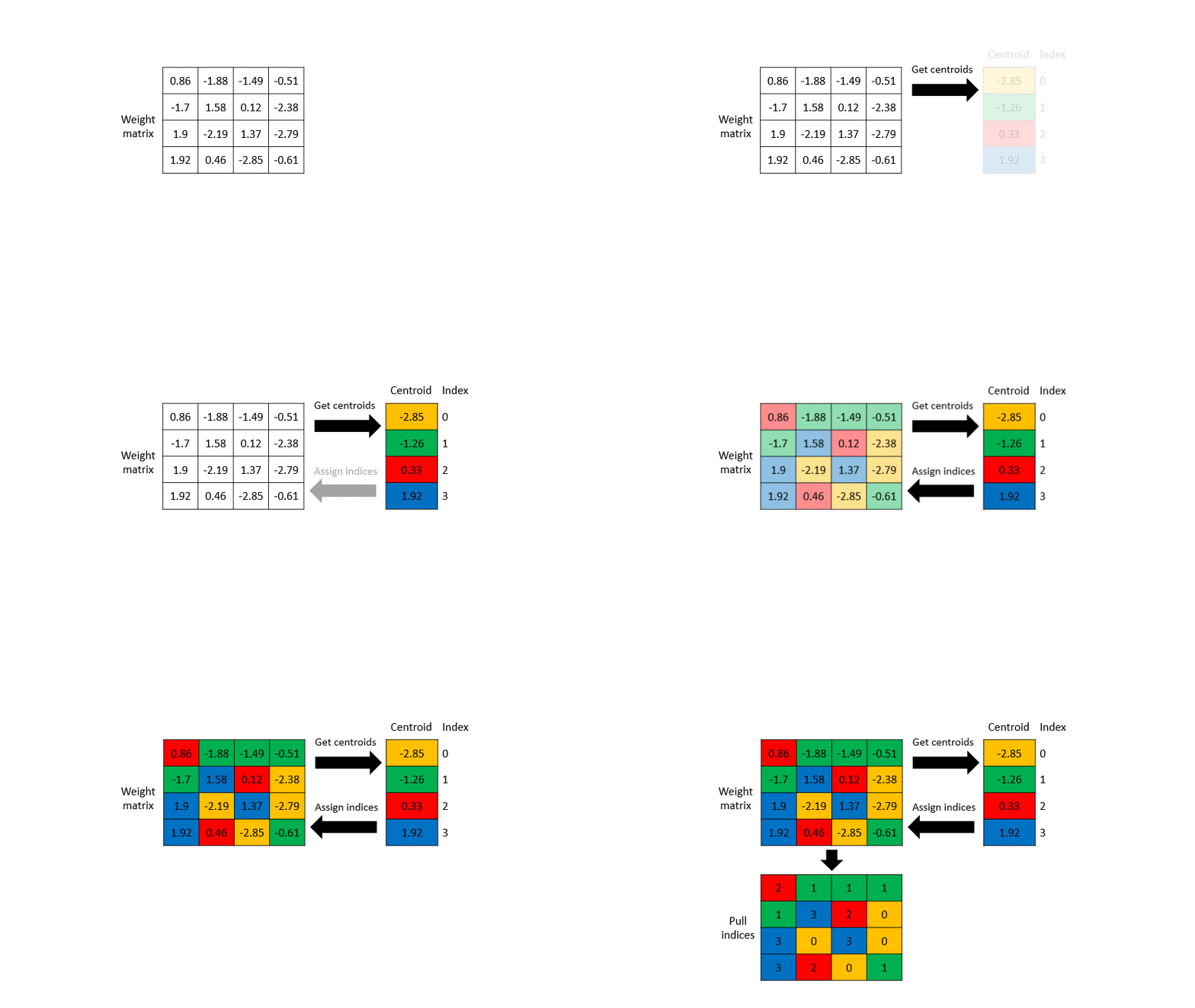
Weight clustering is an optimization algorithm to reduce the storage and network transfer size of your model. The idea in a nutshell is explained in the diagram below.

Here’s an explanation of the diagram. Imagine, for example, that a layer in your model contains a 4×4 matrix of weights (represented by the “weight matrix” above). Each weight is stored using a float32 value. When you save the model, you are storing 16 unique float32 values to disk.

Weight clustering reduces the size of your model by replacing similar weights in a layer with the same value. These values are found by running a clustering algorithm over the model’s trained weights. The user can specify the number of clusters (in this case, 4). This step is shown in “Get centroids” in the diagram above, and the 4 centroid values are shown in the “Centroid” table. Each centroid value has an index (0-3).

Next, each weight in the weight matrix is replaced with its centroid’s index. This step is shown in “Assign indices”. Now, instead of storing the original weight matrix, the weight clustering algorithm can store the modified matrix shown in “Pull indices” (containing the index of the centroid values), and the centroid values themselves.

In this case, we have reduced the size from 16 unique floats, to 4 floats and 16 2-bit indices. The savings increase with larger matrix sizes.

Note that even if we still stored 16 floats, they now have just 4 distinct values. Common compression tools (like zip) can now take advantage of the redundancy in the data to achieve higher compression.

The technical implementation of clustering is derived from Deep Compression: Compressing Deep Neural Networks with Pruning, Trained Quantization and Huffman Coding. See the paper for additional details on the gradient update and weight retrieval.

Clustering is available through a simple Keras API, in which any Keras model (or layer) can be wrapped and fine-tuned. See usage examples below.

Advantages of weight clustering

Weight clustering has an immediate advantage in reducing model storage and transfer size across serialization formats, as a model with shared parameters has a much higher compression rate than one without. This is similar to a sparse (pruned) model, except that the compression benefit is achieved through reducing the number of unique weights, while pruning achieves it through setting weights below a certain threshold to zero. Once a Keras model is clustered, the benefit of the reduced size is available by passing it through any common compression tool.

To further unlock the improvements in memory usage and speed at inference time associated with clustering, specialized run-time or compiler software and dedicated machine learning hardware is required. Examples include the Arm ML Ethos-N driver stack for the Ethos-N processor and the Ethos-U Vela compiler for the Ethos-U processor. Both examples currently require quantizing and converting optimized Keras models to TensorFlow Lite first.

Clustering can be done on its own or as part of a cascaded Deep Compression optimization pipeline to achieve further size reduction and inference speed.

Compression and accuracy results

Experiments were run on several popular models, demonstrating compression benefits of weight clustering. More aggressive optimizations can be applied, but at the cost of accuracy. Though the table below includes measurements for TensorFlow Lite models, similar benefits are observed for other serialization formats such as SavedModel.

The table below demonstrates how clustering was configured to achieve the results. Some models were more prone to accuracy degradation from aggressive clustering, in which case selective clustering was used on layers that are more robust to optimization.

Clustering a model

The clustering API is available in the TensorFlow Model Optimization Toolkit starting from release v0.4.0. To cluster a model, it needs to be fully trained first before passing it to the clustering API. A snippet of full model clustering is shown below.

import tensorflow_model_optimization as tfmot
cluster_weights = tfmot.clustering.keras.cluster_weights


pretrained_model = pretrained_model()

clustering_params = {
'number_of_clusters': 32,
'cluster_centroids_init': tfmot.clustering.keras.CentroidInitialization.LINEAR
}

clustered_model = cluster_weights(pretrained_model, **clustering_params)

# Fine-tune
clustered_model.fit(...)


# Prepare model for serving by removing training-only variables.
model_for_serving = tfmot.clustering.keras.strip_clustering(clustered_model)

...

To cluster select layers in a model, you can apply the same clustering method to those layers when constructing a model.

clustered_model = tf.keras.Sequential([
Dense(...),
cluster_weights(Dense(...,
kernel_initializer=pretrained_weights,
bias_initializer=pretrained_bias),
**clustering_params),
Dense(...)
])

When selectively clustering a layer, it still needs to have been fully trained; therefore, we use the layer’s kernel_initializer parameter to initialize the weights. Using tf.keras.models.clone_model is another option.

Documentation

To learn more about how to use the API, you can try this simple end-to-end clustering example colab to start. A more comprehensive guide with additional tips can be found here.

Acknowledgments

The feature and results presented in this post are the work of many people including the Arm ML Tooling team and our collaborators in Google’s TensorFlow Model Optimization Toolkit team.

From Arm – Anton Kachatkou, Aron Virginas-Tar, Ruomei Yan, Konstantin Sofeikov, Saoirse Stewart, Peng Sun, Elena Zhelezina, Gergely Nagy, Les Bell, Matteo Martincigh, Grant Watson, Diego Russo, Benjamin Klimczak, Thibaut Goetghebuer-Planchon.

From Google – Alan Chiao, Raziel Alvarez
Read More

Efficient PyTorch I/O library for Large Datasets, Many Files, Many GPUs

Efficient PyTorch I/O library for Large Datasets, Many Files, Many GPUs

Data sets are growing bigger every day and GPUs are getting faster. This means there are more data sets for deep learning researchers and engineers to train and validate their models.

  • Many datasets for research in still image recognition are becoming available with 10 million or more images, including OpenImages and Places.
  • million YouTube videos (YouTube 8M) consume about 300 TB in 720p, used for research in object recognition, video analytics, and action recognition.
  • The Tobacco Corpus consists of about 20 million scanned HD pages, useful for OCR and text analytics research.

Although the most commonly encountered big data sets right now involve images and videos, big datasets occur in many other domains and involve many other kinds of data types: web pages, financial transactions, network traces, brain scans, etc.

However, working with the large amount of data sets presents a number of challenges:

  • Dataset Size: datasets often exceed the capacity of node-local disk storage, requiring distributed storage systems and efficient network access.
  • Number of Files: datasets often consist of billions of files with uniformly random access patterns, something that often overwhelms both local and network file systems.
  • Data Rates: training jobs on large datasets often use many GPUs, requiring aggregate I/O bandwidths to the dataset of many GBytes/s; these can only be satisfied by massively parallel I/O systems.
  • Shuffling and Augmentation: training data needs to be shuffled and augmented prior to training.
  • Scalability: users often want to develop and test on small datasets and then rapidly scale up to large datasets.

Traditional local and network file systems, and even object storage servers, are not designed for these kinds of applications. The WebDataset I/O library for PyTorch, together with the optional AIStore server and Tensorcom RDMA libraries, provide an efficient, simple, and standards-based solution to all these problems. The library is simple enough for day-to-day use, is based on mature open source standards, and is easy to migrate to from existing file-based datasets.

Using WebDataset is simple and requires little effort, and it will let you scale up the same code from running local experiments to using hundreds of GPUs on clusters or in the cloud with linearly scalable performance. Even on small problems and on your desktop, it can speed up I/O tenfold and simplifies data management and processing of large datasets. The rest of this blog post tells you how to get started with WebDataset and how it works.

The WebDataset Library

The WebDataset library provides a simple solution to the challenges listed above. Currently, it is available as a separate library (github.com/tmbdev/webdataset), but it is on track for being incorporated into PyTorch (see RFC 38419). The WebDataset implementation is small (about 1500 LOC) and has no external dependencies.

Instead of inventing a new format, WebDataset represents large datasets as collections of POSIX tar archive files consisting of the original data files. The WebDataset library can use such tar archives directly for training, without the need for unpacking or local storage.

WebDataset scales perfectly from small, local datasets to petascale datasets and training on hundreds of GPUs and allows data to be stored on local disk, on web servers, or dedicated file servers. For container-based training, WebDataset eliminates the need for volume plugins or node-local storage. As an additional benefit, datasets need not be unpacked prior to training, simplifying the distribution and use of research data.

WebDataset implements PyTorch’s IterableDataset interface and can be used like existing DataLoader-based code. Since data is stored as files inside an archive, existing loading and data augmentation code usually requires minimal modification.

The WebDataset library is a complete solution for working with large datasets and distributed training in PyTorch (and also works with TensorFlow, Keras, and DALI via their Python APIs). Since POSIX tar archives are a standard, widely supported format, it is easy to write other tools for manipulating datasets in this format. E.g., the tarp command is written in Go and can shuffle and process training datasets.

Benefits

The use of sharded, sequentially readable formats is essential for very large datasets. In addition, it has benefits in many other environments. WebDataset provides a solution that scales well from small problems on a desktop machine to very large deep learning problems in clusters or in the cloud. The following table summarizes some of the benefits in different environments.

Environment Benefits of WebDataset
Local Cluster with AIStore AIStore can be deployed easily as K8s containers and offers linear scalability and near 100% utilization of network and I/O bandwidth. Suitable for petascale deep learning.
Cloud Computing WebDataset deep learning jobs can be trained directly against datasets stored in cloud buckets; no volume plugins required. Local and cloud jobs work identically. Suitable for petascale learning.
Local Cluster with existing distributed FS or object store WebDataset’s large sequential reads improve performance with existing distributed stores and eliminate the need for dedicated volume plugins.
Educational Environments WebDatasets can be stored on existing web servers and web caches, and can be accessed directly by students by URL
Training on Workstations from Local Drives Jobs can start training as the data still downloads. Data doesn’t need to be unpacked for training. Ten-fold improvements in I/O performance on hard drives over random access file-based datasets.
All Environments Datasets are represented in an archival format and contain metadata such as file types. Data is compressed in native formats (JPEG, MP4, etc.). Data management, ETL-style jobs, and data transformations and I/O are simplified and easily parallelized.

We will be adding more examples giving benchmarks and showing how to use WebDataset in these environments over the coming months.

High-Performance

For high-performance computation on local clusters, the companion open-source AIStore server provides full disk to GPU I/O bandwidth, subject only to hardware constraints. This Bigdata 2019 Paper contains detailed benchmarks and performance measurements. In addition to benchmarks, research projects at NVIDIA and Microsoft have used WebDataset for petascale datasets and billions of training samples.

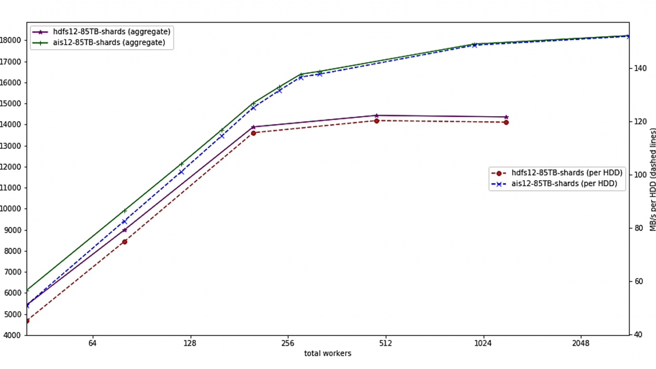
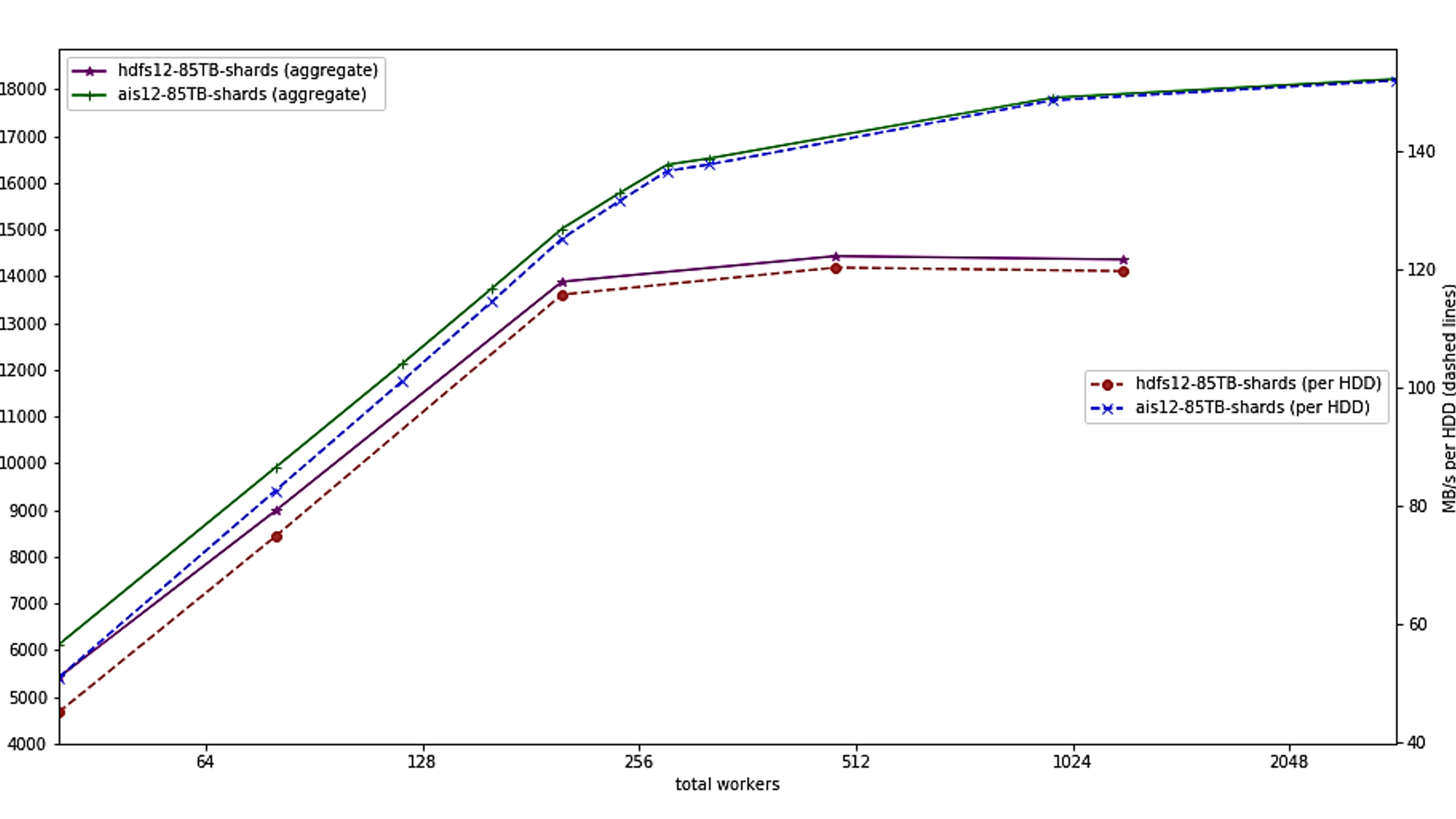
Below is a benchmark of AIStore with WebDataset clients using 10 server nodes and 120 rotational drives each.

The left axis shows the aggregate bandwidth from the cluster, while the right scale shows the measured per drive I/O bandwidth. WebDataset and AIStore scale linearly to about 300 clients, at which point they are increasingly limited by the maximum I/O bandwidth available from the rotational drives (about 150 MBytes/s per drive). For comparison, HDFS is shown. HDFS uses a similar approach to AIStore/WebDataset and also exhibits linear scaling up to about 192 clients; at that point, it hits a performance limit of about 120 MBytes/s per drive, and it failed when using more than 1024 clients. Unlike HDFS, the WebDataset-based code just uses standard URLs and HTTP to access data and works identically with local files, with files stored on web servers, and with AIStore. For comparison, NFS in similar experiments delivers about 10-20 MBytes/s per drive.

Storing Datasets in Tar Archives

The format used for WebDataset is standard POSIX tar archives, the same archives used for backup and data distribution. In order to use the format to store training samples for deep learning, we adopt some simple naming conventions:

  • datasets are POSIX tar archives
  • each training sample consists of adjacent files with the same basename
  • shards are numbered consecutively

For example, ImageNet is stored in 1282 separate 100 Mbyte shards with names pythonimagenet-train-000000.tar to imagenet-train-001281.tar, the contents of the first shard are:

-r--r--r-- bigdata/bigdata      3 2020-05-08 21:23 n03991062_24866.cls
-r--r--r-- bigdata/bigdata 108611 2020-05-08 21:23 n03991062_24866.jpg
-r--r--r-- bigdata/bigdata      3 2020-05-08 21:23 n07749582_9506.cls
-r--r--r-- bigdata/bigdata 129044 2020-05-08 21:23 n07749582_9506.jpg
-r--r--r-- bigdata/bigdata      3 2020-05-08 21:23 n03425413_23604.cls
-r--r--r-- bigdata/bigdata 106255 2020-05-08 21:23 n03425413_23604.jpg
-r--r--r-- bigdata/bigdata      3 2020-05-08 21:23 n02795169_27274.cls

WebDataset datasets can be used directly from local disk, from web servers (hence the name), from cloud storage and object stores, just by changing a URL. WebDataset datasets can be used for training without unpacking, and training can even be carried out on streaming data, with no local storage.

Shuffling during training is important for many deep learning applications, and WebDataset performs shuffling both at the shard level and at the sample level. Splitting of data across multiple workers is performed at the shard level using a user-provided shard_selection function that defaults to a function that splits based on get_worker_info. (WebDataset can be combined with the tensorcom library to offload decompression/data augmentation and provide RDMA and direct-to-GPU loading; see below.)

Code Sample

Here are some code snippets illustrating the use of WebDataset in a typical PyTorch deep learning application (you can find a full example at http://github.com/tmbdev/pytorch-imagenet-wds.

import webdataset as wds
import ...

sharedurl = "/imagenet/imagenet-train-{000000..001281}.tar"

normalize = transforms.Normalize(
  mean=[0.485, 0.456, 0.406],
  std=[0.229, 0.224, 0.225])

preproc = transforms.Compose([
  transforms.RandomResizedCrop(224),
  transforms.RandomHorizontalFlip(),
  transforms.ToTensor(),
  normalize,
])

dataset = (
  wds.Dataset(sharedurl)
  .shuffle(1000)
  .decode("pil")
  .rename(image="jpg;png", data="json")
  .map_dict(image=preproc)
  .to_tuple("image", "data")
)

loader = torch.utils.data.DataLoader(dataset, batch_size=64, num_workers=8)

for inputs, targets in loader:
  ...

This code is nearly identical to the file-based I/O pipeline found in the PyTorch Imagenet example: it creates a preprocessing/augmentation pipeline, instantiates a dataset using that pipeline and a data source location, and then constructs a DataLoader instance from the dataset.

WebDataset uses a fluent API for a configuration that internally builds up a processing pipeline. Without any added processing stages, In this example, WebDataset is used with the PyTorch DataLoader class, which replicates DataSet instances across multiple threads and performs both parallel I/O and parallel data augmentation.

WebDataset instances themselves just iterate through each training sample as a dictionary:

# load from a web server using a separate client process
sharedurl = "pipe:curl -s http://server/imagenet/imagenet-train-{000000..001281}.tar"

dataset = wds.Dataset(sharedurl)

for sample in dataset:
  # sample["jpg"] contains the raw image data
  # sample["cls"] contains the class
  ...

For a general introduction to how we handle large scale training with WebDataset, see these YouTube videos.

Related Software

  • AIStore is an open-source object store capable of full-bandwidth disk-to-GPU data delivery (meaning that if you have 1000 rotational drives with 200 MB/s read speed, AIStore actually delivers an aggregate bandwidth of 200 GB/s to the GPUs). AIStore is fully compatible with WebDataset as a client, and in addition understands the WebDataset format, permitting it to perform shuffling, sorting, ETL, and some map-reduce operations directly in the storage system. AIStore can be thought of as a remix of a distributed object store, a network file system, a distributed database, and a GPU-accelerated map-reduce implementation.

  • tarp is a small command-line program for splitting, merging, shuffling, and processing tar archives and WebDataset datasets.

  • tensorcom is a library supporting distributed data augmentation and RDMA to GPU.

  • webdataset-examples contains an example (and soon more examples) of how to use WebDataset in practice.

  • Bigdata 2019 Paper with Benchmarks

Check out the library and provide your feedback for RFC 38419.

Read More

Data systems that learn to be better

Big data has gotten really, really big: By 2025, all the world’s data will add up to an estimated 175 trillion gigabytes. For a visual, if you stored that amount of data on DVDs, it would stack up tall enough to circle the Earth 222 times. 

One of the biggest challenges in computing is handling this onslaught of information while still being able to efficiently store and process it. A team from MIT’s Computer Science and Artificial Intelligence Laboratory (CSAIL) believe that the answer rests with something called “instance-optimized systems.”  

Traditional storage and database systems are designed to work for a wide range of applications because of how long it can take to build them — months or, often, several years. As a result, for any given workload such systems provide performance that is good, but usually not the best. Even worse, they sometimes require administrators to painstakingly tune the system by hand to provide even reasonable performance. 

In contrast, the goal of instance-optimized systems is to build systems that optimize and partially re-organize themselves for the data they store and the workload they serve. 

“It’s like building a database system for every application from scratch, which is not economically feasible with traditional system designs,” says MIT Professor Tim Kraska. 

As a first step toward this vision, Kraska and colleagues developed Tsunami and Bao. Tsunami uses machine learning to automatically re-organize a dataset’s storage layout based on the types of queries that its users make. Tests show that it can run queries up to 10 times faster than state-of-the-art systems. What’s more, its datasets can be organized via a series of “learned indexes” that are up to 100 times smaller than the indexes used in traditional systems. 

Kraska has been exploring the topic of learned indexes for several years, going back to his influential work with colleagues at Google in 2017. 

Harvard University Professor Stratos Idreos, who was not involved in the Tsunami project, says that a unique advantage of learned indexes is their small size, which, in addition to space savings, brings substantial performance improvements.

“I think this line of work is a paradigm shift that’s going to impact system design long-term,” says Idreos. “I expect approaches based on models will be one of the core components at the heart of a new wave of adaptive systems.”

Bao, meanwhile, focuses on improving the efficiency of query optimization through machine learning. A query optimizer rewrites a high-level declarative query to a query plan, which can actually be executed over the data to compute the result to the query. However, often there exists more than one query plan to answer any query; picking the wrong one can cause a query to take days to compute the answer, rather than seconds. 

Traditional query optimizers take years to build, are very hard to maintain, and, most importantly, do not learn from their mistakes. Bao is the first learning-based approach to query optimization that has been fully integrated into the popular database management system PostgreSQL. Lead author Ryan Marcus, a postdoc in Kraska’s group, says that Bao produces query plans that run up to 50 percent faster than those created by the PostgreSQL optimizer, meaning that it could help to significantly reduce the cost of cloud services, like Amazon’s Redshift, that are based on PostgreSQL.

By fusing the two systems together, Kraska hopes to build the first instance-optimized database system that can provide the best possible performance for each individual application without any manual tuning. 

The goal is to not only relieve developers from the daunting and laborious process of tuning database systems, but to also provide performance and cost benefits that are not possible with traditional systems.

Traditionally, the systems we use to store data are limited to only a few storage options and, because of it, they cannot provide the best possible performance for a given application. What Tsunami can do is dynamically change the structure of the data storage based on the kinds of queries that it receives and create new ways to store data, which are not feasible with more traditional approaches.

Johannes Gehrke, a managing director at Microsoft Research who also heads up machine learning efforts for Microsoft Teams, says that his work opens up many interesting applications, such as doing so-called “multidimensional queries” in main-memory data warehouses. Harvard’s Idreos also expects the project to spur further work on how to maintain the good performance of such systems when new data and new kinds of queries arrive.

Bao is short for “bandit optimizer,” a play on words related to the so-called “multi-armed bandit” analogy where a gambler tries to maximize their winnings at multiple slot machines that have different rates of return. The multi-armed bandit problem is commonly found in any situation that has tradeoffs between exploring multiple different options, versus exploiting a single option — from risk optimization to A/B testing.

“Query optimizers have been around for years, but they often make mistakes, and usually they don’t learn from them,” says Kraska. “That’s where we feel that our system can make key breakthroughs, as it can quickly learn for the given data and workload what query plans to use and which ones to avoid.”

Kraska says that in contrast to other learning-based approaches to query optimization, Bao learns much faster and can outperform open-source and commercial optimizers with as little as one hour of training time.In the future, his team aims to integrate Bao into cloud systems to improve resource utilization in environments where disk, RAM, and CPU time are scarce resources.

“Our hope is that a system like this will enable much faster query times, and that people will be able to answer questions they hadn’t been able to answer before,” says Kraska.

A related paper about Tsunami was co-written by Kraska, PhD students Jialin Ding and Vikram Nathan, and MIT Professor Mohammad Alizadeh. A paper about Bao was co-written by Kraska, Marcus, PhD students Parimarjan Negi and Hongzi Mao, visiting scientist Nesime Tatbul, and Alizadeh.

The work was done as part of the Data System and AI Lab (DSAIL@CSAIL), which is sponsored by Intel, Google, Microsoft, and the U.S. National Science Foundation. 

Read More

Layerwise learning for Quantum Neural Networks

Layerwise learning for Quantum Neural Networks

Posted by Andrea Skolik, Volkswagen AG and Leiden University

In early March, Google released TensorFlow Quantum (TFQ) together with the University of Waterloo and Volkswagen AG. TensorFlow Quantum is a software framework for quantum machine learning (QML) which allows researchers to jointly use functionality from Cirq and TensorFlow. Both Cirq and TFQ are aimed at simulating noisy intermediate-scale quantum (NISQ) devices that are currently available, but are still in an experimental stage and therefore come without error correction and suffer from noisy outputs.

In this article, we introduce a training strategy that addresses vanishing gradients in quantum neural networks (QNNs), and makes better use of the resources provided by a NISQ device. If you’d like to play with the code for this example yourself, check out the notebook on layerwise learning in the TFQ research repository, where we train a QNN on a simulated quantum computer!

Quantum Neural Networks

Training a QNN is not that much different from training a classical neural network, just that instead of optimizing network weights, we optimize the parameters of a quantum circuit. A quantum circuit looks like the following:
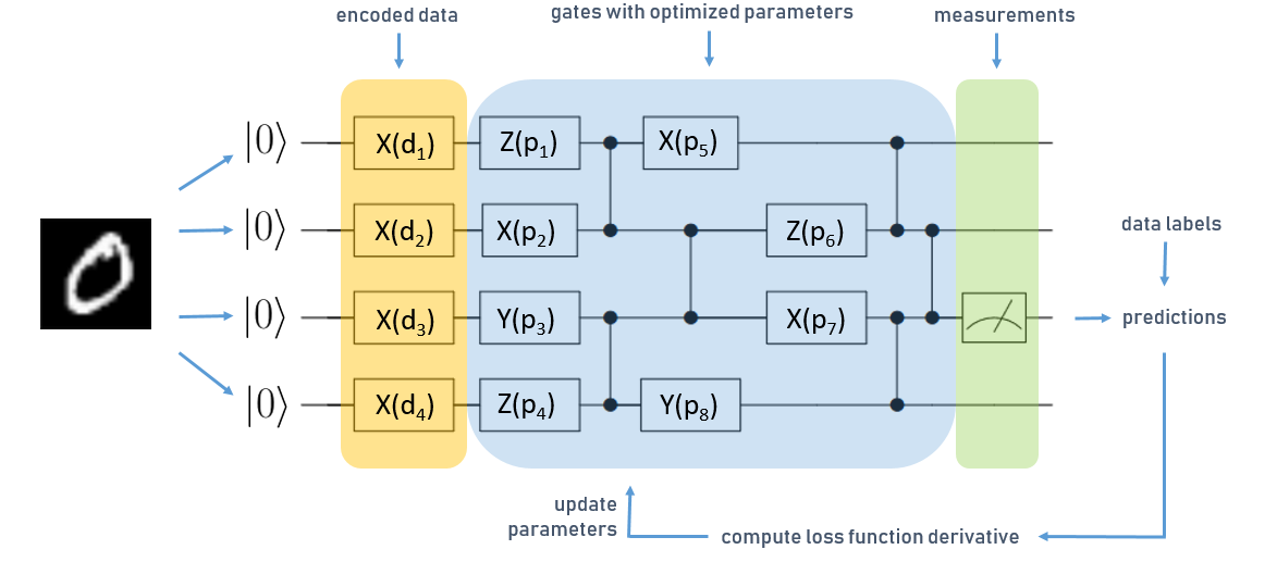
Simplified QNN for a classification task with four qubits

The circuit is read from left to right, and each horizontal line corresponds to one qubit in the register of the quantum computer, each initialized in the zero state. The boxes denote parametrized operations (or “gates”) on qubits which are executed sequentially. In this case we have three different types of operations, X, Y, and Z. Vertical lines denote two-qubit gates, which can be used to generate entanglement in the QNN – one of the resources that lets quantum computers outperform their classical counterparts. We denote one layer as one operation on each qubit, followed by a sequence of gates that connect pairs of qubits to generate entanglement.

The figure above shows a simplified QNN for learning classification of MNIST digits.

First, we have to encode the data set into quantum states. We do this by using a data encoding layer, marked orange in the figure above. In this case, we transform our input data into a vector, and use the vector values as parameters d for the data encoding layers’ operations. Based on this input, we execute the part of the circuit marked in blue, which represents the trainable gates of our QNN, denoted by p.

The last operation in the quantum circuit is a measurement. During computation, the quantum device performs operations on superpositions of classical bitstrings. When we perform a readout on the circuit, the superposition state collapses to one classical bitstring, which is the output of the computation that we get. The so-called collapse of the quantum state is probabilistic, to get a deterministic outcome we average over multiple measurement outcomes.

In the above picture, marked in green, we perform measurements on the third qubit and use these to predict labels for our MNIST examples. We compare this to the true data label and compute gradients of a loss function just like in a classical NN. These types of QNNs are called “hybrid quantum-classical”, as the parameter optimization is handled by a classical computer, using e.g. the Adam optimizer.

Vanishing gradients, aka barren plateaus

It turns out that QNNs also suffer from vanishing gradients, just like classical NNs. Since the reason for vanishing gradients in QNNs is fundamentally different from classical NNs, a new term has been adopted for them: barren plateaus. Covering all details of this important phenomenon is out of the scope of this article, so we refer the interested reader to the paper that first introduced barren plateaus in QNN training landscapes or this tutorial on barren plateaus on the TFQ site for a hands-on example.

In short, barren plateaus occur when quantum circuits are initialized randomly – in the circuit illustrated above this means picking operations and their parameters at random. This is a fundamental problem for training parametrized quantum circuits, and gets worse as the number of qubits and the number of layers in a circuit grows, as we can see in the figure below.
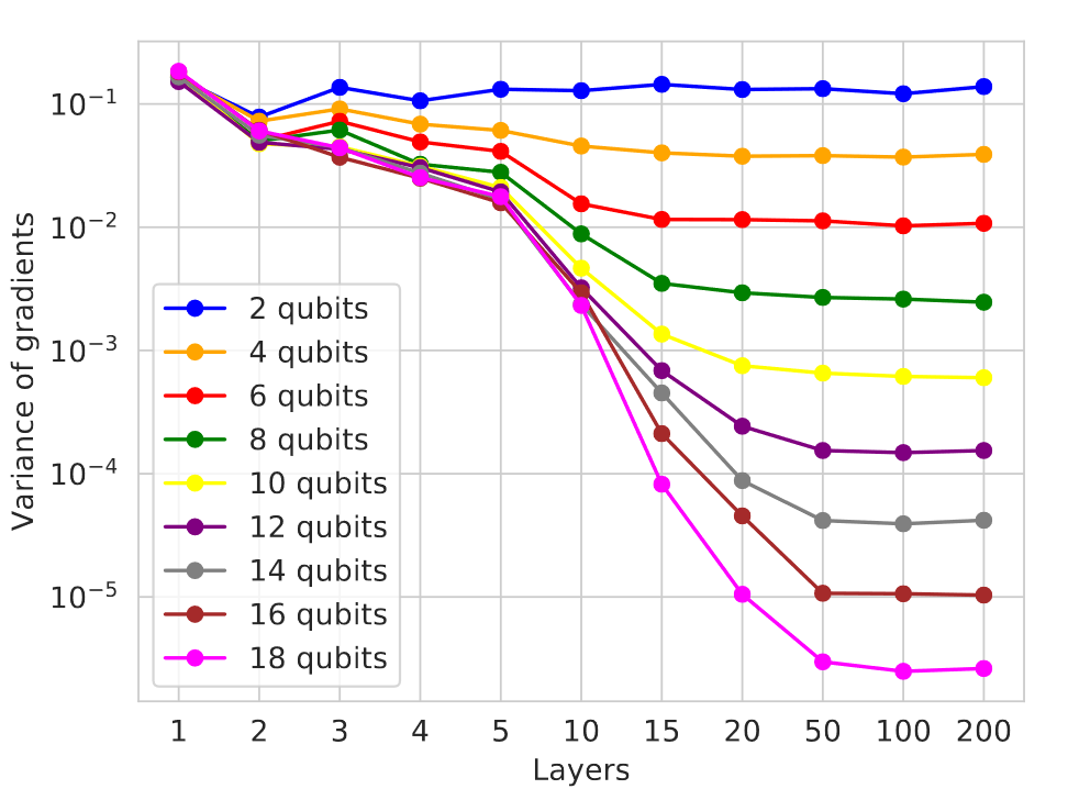
Variance of gradients decays as a function of the number of qubits and layers in a random circuit

For the algorithm we introduce below, the key thing to understand here is that the more layers we add to a circuit, the smaller the variance in gradients will get. On the other hand, similarly to classical NNs, the QNN’s representational capacity also increases with its depth. The problem here is that in addition, the optimization landscape flattens in many places as we increase the circuit’s size, so it gets harder to find even a local minimum.

Remember that for QNNs, outputs are estimated from taking the average over a number of measurements. The smaller the quantity we want to estimate, the more measurements we will need to get an accurate result. If these quantities are much smaller compared to the effects caused by measurement uncertainty or hardware noise, they can’t be reliably determined and the circuit optimization will basically turn into a random walk.

To successfully train a QNN, we have to avoid random initialization of the parameters, and also have to stop the QNN from randomizing during training as its gradients get smaller, for example when it approaches a local minimum. For this, we can either limit the architecture of the QNN (e.g. by picking certain gate configurations, which requires tuning the architecture to the task at hand), or control the updates to parameters such that they won’t become random.

Layerwise learning

In our paper Layerwise learning for quantum neural networks, which is joint work by the Volkswagen Data:Lab (Andrea Skolik, Patrick van der Smagt, Martin Leib) and Google AI Quantum (Jarrod R. McClean, Masoud Mohseni), we introduce an approach to avoid initialization on a plateau as well as the network ending up on a plateau during training. Let’s look at an example of layerwise learning (LL) in action, on the learning task of binary classification of MNIST digits. First, we need to define the structure of the layers we want to stack. As we make no assumptions about the learning task at hand, we choose the same layout for our layers as in the figure above: one layer consists of random gates on each qubit initialized with zero, and two-qubit gates which connect qubits to enable generation of entanglement.

We designate a number of start layers, in this case only one, which will always stay active during training, and specify the number of epochs to train each set of layers. Two other hyperparameters are the number of new layers we add in each step, and the number of layers that are maximally trained at once. Here we choose a configuration where we add two layers in each step, and freeze the parameters of all previous layers, except the start layer, such that we only train three layers in each step. We train each set of layers for 10 epochs, and repeat this procedure ten times until our circuit consists of 21 layers overall. By doing this, we utilize the fact that shallow circuits produce larger gradients compared to deeper ones, and with this avoid initializing on a plateau.

This provides us with a good starting point in the optimization landscape to continue training larger contiguous sets of layers. As another hyperparameter, we define the percentage of layers we train together in the second phase of the algorithm. Here, we choose to split the circuit in half, and alternatingly train both parts, where the parameters of the inactive parts are always frozen. We call one training sequence where all partitions have been trained once a sweep, and we perform sweeps over this circuit until the loss converges. When the full set of parameters is always trained, which we will refer to as “complete depth learning” (CDL), one bad update step can affect the whole circuit and lead it into a random configuration and therefore a barren plateau, from which it cannot escape anymore.

Let’s compare our training strategy to CDL, which is one of the standard techniques used to train QNNs. To get a fair comparison, we use exactly the same circuit architecture as the one generated by the LL strategy before, but now update all parameters simultaneously in each step. To give CDL a chance to train, we optimize the parameters with zero instead of randomly. As we don’t have access to a real quantum computer yet, we simulate the probabilistic outputs of the QNN, and choose a relatively low value for the number of measurements that we use to estimate each prediction the QNN makes – which is 10 in this case. Assuming a 10kHZ sampling rate on a real quantum computer, we can estimate the experimental wall-clock time of our training runs as shown below:
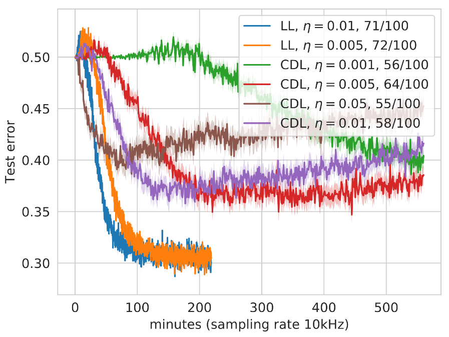
Comparison of layerwise- and complete depth learning with different learning rates η. We trained 100 circuits for each configuration, and averaged over those that achieved a final test error lower than 0.5 (number of succeeding runs in legend).

With this small number of measurements, we can investigate the effects of the different gradient magnitudes of the LL and CDL approaches: if gradient values are larger, we get more information out of 10 measurements than for smaller values. The less information we have to perform our parameter updates, the higher the variance in the loss, and the risk to perform an erroneous update that will randomize the updated parameters and lead the QNN onto a plateau. This variance can be lowered by choosing a smaller learning rate, so we compare LL and CDL strategies with different learning rates in the figure above.

Notably, the test error of CDL runs increases with the runtime, which might look like overfitting at first. However, each curve in this figure is averaged over many runs, and what is actually happening here is that more and more CDL runs randomize during training, unable to recover. In the legend we show that a much larger fraction of LL runs achieved a classification error on the test set lower than 0.5 compared to CDL, and also did it in less time.

In summary, layerwise learning increases the probability of successfully training a QNN with overall better generalization error in less training time, which is especially valuable on NISQ devices. For more details on the implementation and theory of layerwise learning, check out our recent paper!

If you’d like to learn more about quantum computing and quantum machine learning in general, there are some additional resources below:

Read More

Machine learning best practices in financial services

Machine learning best practices in financial services

We recently published a new whitepaper, Machine Learning Best Practices in Financial Services, that outlines security and model governance considerations for financial institutions building machine learning (ML) workflows. The whitepaper discusses common security and compliance considerations and aims to accompany a hands-on demo and workshop that walks you through an end-to-end example. Although the whitepaper focuses on financial services considerations, much of the information around authentication and access management, data and model security, and ML operationalization (MLOps) best practices may be applicable to other regulated industries, such as healthcare.

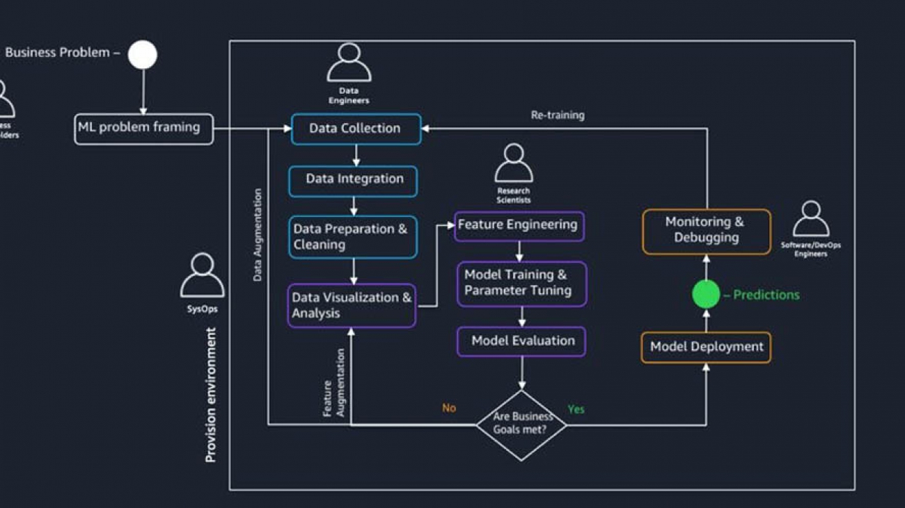
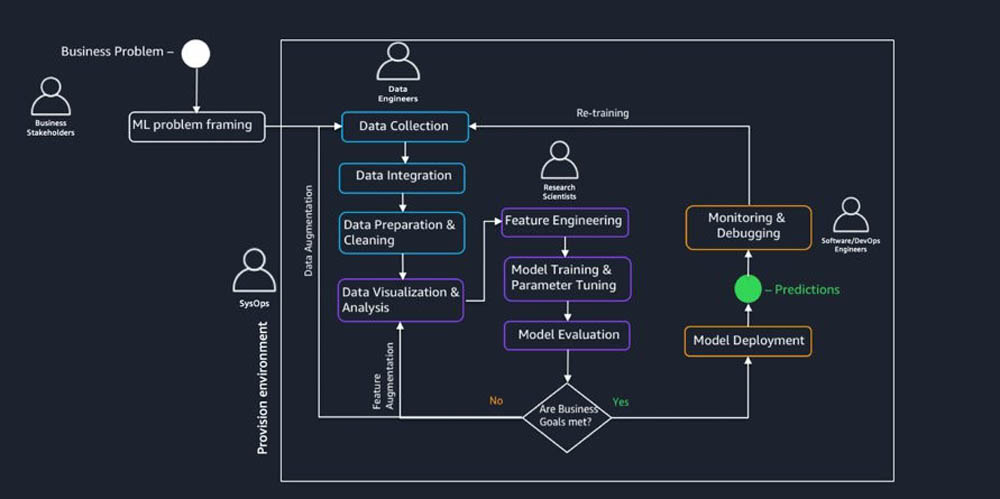
A typical ML workflow, as shown in the following diagram, involves multiple stakeholders. To successfully govern and operationalize this workflow, you should collaborate across multiple teams, including business stakeholders, sysops administrators, data engineers, and software and devops engineers.

In the whitepaper, we discuss considerations for each team and also provide examples and illustrations of how you can use Amazon SageMaker and other AWS services to build, train, and deploy ML workloads. More specifically, based on feedback from customers running workloads in regulated environments, we cover the following topics:

  • Provisioning a secure ML environment – This includes the following:
    • Compute and network isolation – How to deploy Amazon SageMaker in a customer’s private network, with no internet connectivity.
    • Authentication and authorization – How to authenticate users in a controlled fashion and authorize these users based on their AWS Identity and Access Management (IAM) permissions, with no multi-tenancy.
    • Data protection – How to encrypt data in transit and at rest with customer-provided encryption keys.
    • Auditability – How to audit, prevent, and detect who did what at any given point in time to help identify and protect against malicious activities.
  • Establishing ML governance – This includes the following:
    • Traceability – Methods to trace ML model lineage from data preparation, model development, and training iterations, and how to audit who did what at any given point in time.
    • Explainability and interpretability –Methods that may help explain and interpret the trained model and obtain feature importance.
    • Model monitoring – How to monitor your model in production to protect against data drift, and automatically react to rules that you define.
    • Reproducibility – How to reproduce the ML model based on model lineage and the stored artifacts.
  • Operationalizing ML workloads – This includes the following:
    • Model development workload – How to build automated and manual review processes in the dev environment.
    • Preproduction workload – How to build automated CI/CD pipelines using the AWS CodeStar suite and AWS Step Functions.
    • Production and continuous monitoring workload – How to combine continuous deployment and automated model monitoring.
    • Tracking and alerting – How to track model metrics (operational and statistical) and alert appropriate users if anomalies are detected.

Provisioning a secure ML environment

A well-governed and secure ML workflow begins with establishing a private and isolated compute and network environment. This may be especially important in regulated industries, particularly when dealing with PII data for model building or training. The Amazon Virtual Private Cloud (VPC) that hosts Amazon SageMaker and its associated components, such as Jupyter notebooks, training instances, and hosting instances, should be deployed in a private network with no internet connectivity.

Furthermore, you can associate these Amazon SageMaker resources with your VPC environment, which allows you to apply network-level controls, such as security groups to govern access to Amazon SageMaker resources and control ingress and egress of data into and out of the environment. You can establish connectivity between Amazon SageMaker and other AWS services, such as Amazon Simple Storage Service (Amazon S3), using VPC endpoints or AWS PrivateLink. The following diagram illustrates a suggested reference architecture of a secure Amazon SageMaker deployment.

The next step is to ensure that only authorized users can access the appropriate AWS services. IAM can help you create preventive controls for many aspects of your ML environment, including access to Amazon SageMaker resources, your data in Amazon S3, and API endpoints. You can access AWS services using a RESTful API, and every API call is authorized by IAM. You grant explicit permissions through IAM policy documents, which specify the principal (who), the actions (API calls), and the resources (such as Amazon S3 objects) that are allowed, as well as the conditions under which the access is granted. For a deeper dive into building secure environments for financial services as well as other well-architected pillars, also refer to this whitepaper.

In addition, as ML environments may contain sensitive data and intellectual property, the third consideration for a secure ML environment is data encryption. We recommend that you enable data encryption both at rest and in transit with your own encryption keys. And lastly, another consideration for a well-governed and secure ML environment is a robust and transparent audit trail that logs all access and changes to the data and models, such as a change in the model configuration or the hyperparameters. More details on all those fronts are included in the whitepaper.

To enable self-service provisioning and automation, administrators can use tools such as the AWS Service Catalog to create these secure environments in a repeatable manner for their data scientists. This way, data scientists can simply log in to a secure portal using AWS Single Sign-On, and create a secure Jupyter notebook environment provisioned for their use with appropriate security guardrails in place.

Establishing ML governance

In this section of the whitepaper, we discuss the considerations around ML governance, which includes four key aspects: traceability, explainability, real-time model monitoring, and reproducibility. The financial services industry has various compliance and regulatory obligations that may touch on these aspects of ML governance. You should review and understand those obligations with your legal counsel, compliance personnel, and other stakeholders involved in the ML process.

As an example, if Jane Smith is denied a bank loan, the lender may be required to explain how that decision was made in order to comply with regulatory requirements. If the financial services industry customer is using ML as part of the loan review process, the prediction made by the ML model may need to be interpreted or explained in order to meet these requirements. Generally, an ML model’s interpretability or explainability refers to people’s ability to understand and explain the processes that the model uses to arrive at its predictions. It is also important to note that many ML models make predictions of a likely answer, rather than the answer itself. Therefore, it may be appropriate to have human review of predictions made by ML models before any action is taken. The model may also need to be monitored, so that if the underlying data changes, the model is periodically retrained on new data. Finally, the ML model may need to be reproducible, such that if the steps leading to the model’s output are retraced, the model outputs don’t change.

Operationalizing ML workloads

In the final section, we discuss some best practices around operationalizing ML workloads. We begin with a high-level discussion and then dive deeper into a specific architecture that uses AWS native tools and services. In addition to the process of deploying models, or what in traditional software deployments is referred to as CI/CD (continuous integration/deployment), deploying ML models into production for regulated industries may have additional implications from an implementation perspective.

The following diagram captures some of the high-level requirements that an enterprise ML platform might have to address guidelines around governance, auditing, logging, and reporting:

  • A data lake for managing raw data and associated metadata
  • A feature store for managing ML features and associated metadata (mapping from raw data to generated features such as one-hot encodings or scaling transformations)
  • A model and container registry containing trained model artifacts and associated metadata (such as hyperparameters, training times, and dependencies)
  • A code repository (such as Git, AWS CodeCommit, or Artifactory) for maintaining and versioning source code
  • A pipeline registry to version and maintain training and deployment pipelines
  • Logging tools for maintaining access logs
  • Production monitoring and performance logs
  • Tools for auditing and reporting

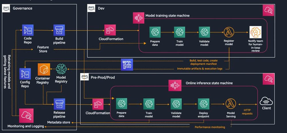
The following diagram illustrates a specific implementation that uses AWS native tools and services. Although several scheduling and orchestration tools are on the market, such as Airflow or Jenkins, for concreteness, we focus predominantly on Step Functions.

In the whitepaper, we dive deeper into each part of the preceding diagram, and more specifically into the following workloads:

  • Model development
  • Pre-production
  • Production and continuous monitoring

Summary

The Machine Learning Best Practices in Financial Services whitepaper is available here. Start using it today to help illustrate how you can build secure and well-governed ML workflows and feel free to reach out to the authors if you have any questions. As you progress on your journey, also refer to this whitepaper for a lens on the AWS well-architected principles applied to machine learning workloads. You can also use the video demo walkthrough, and the following two workshops:


About the authors

Stefan Natu is a Sr. Machine Learning Specialist at Amazon Web Services. He is focused on helping financial services customers build and operationalize end-to-end machine learning solutions on AWS. His academic background is in theoretical physics, and in the past, he worked on a number of data science problems in retail and energy verticals. In his spare time, he enjoys reading machine learning blogs, traveling, playing the guitar, and exploring the food scene in New York City.


Kosti Vasilakakis is a Sr. Business Development Manager for Amazon SageMaker, the AWS fully managed service for end-to-end machine learning, and he focuses on helping financial services and technology companies achieve more with ML. He spearheads curated workshops, hands-on guidance sessions, and pre-packaged open-source solutions to ensure that customers build better ML models quicker and safer. Outside of work, he enjoys traveling the world, philosophizing, and playing tennis.


Alvin Huang is a Capital Markets Specialist for Worldwide Financial Services Business Development at Amazon Web Services with a focus on data lakes and analytics, and artificial intelligence and machine learning. Alvin has over 19 years of experience in the financial services industry, and prior to joining AWS, he was an Executive Director at J.P. Morgan Chase & Co, where he managed the North America and Latin America trade surveillance teams and led the development of global trade surveillance. Alvin also teaches a Quantitative Risk Management course at Rutgers University and serves on the Rutgers Mathematical Finance Master’s program (MSMF) Advisory Board.


David Ping is a Principal Machine Learning Architect and Sr. Manager of AI/ML Solutions Architecture at Amazon Web Services. He helps enterprise customers build and operate machine learning solutions on AWS. David enjoys hiking and following the latest machine learning advancement.
 

Read More

Mass General’s Martinos Center Adopts AI for COVID, Radiology Research

Mass General’s Martinos Center Adopts AI for COVID, Radiology Research

Academic medical centers worldwide are building new AI tools to battle COVID-19 —  including at Mass General, where one center is adopting NVIDIA DGX A100 AI systems to accelerate its work.

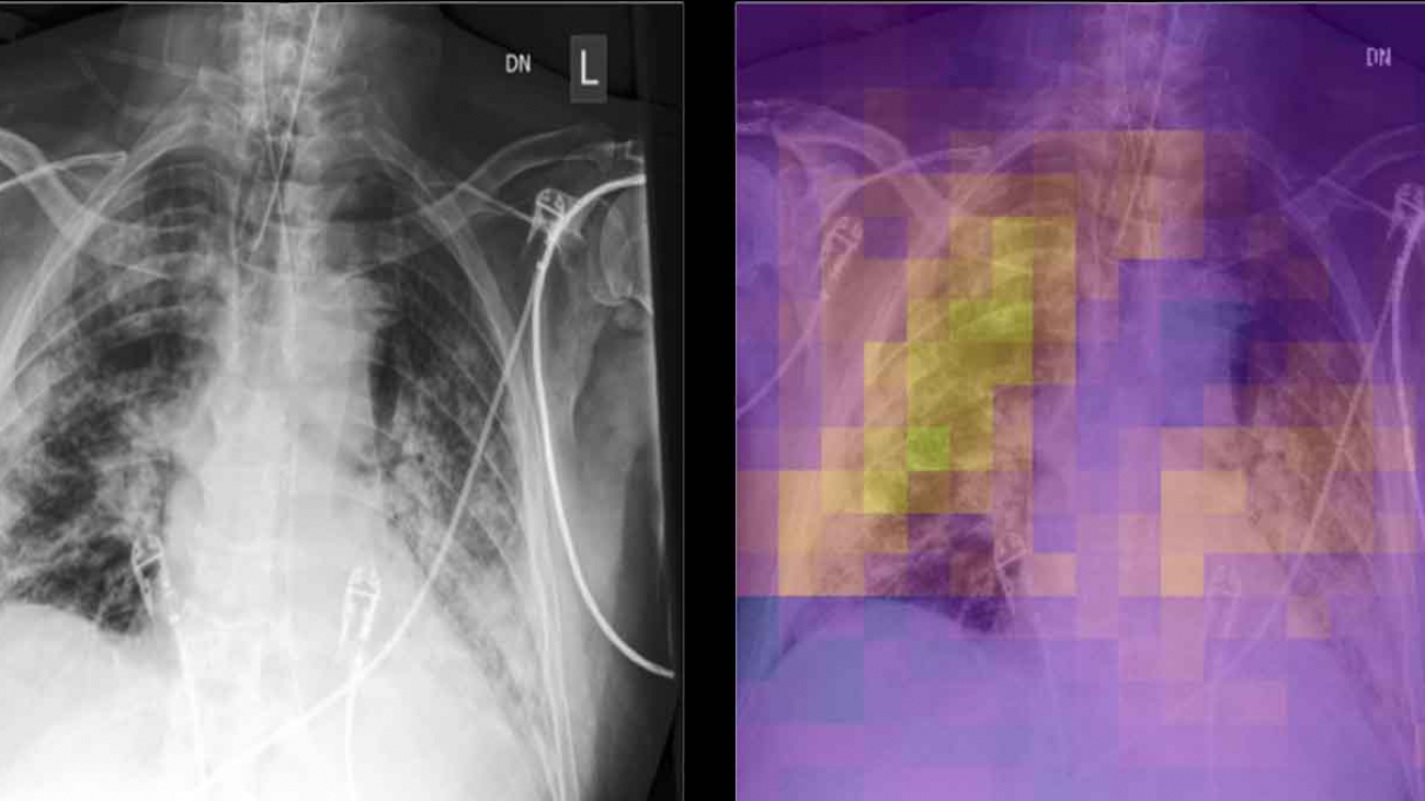
Researchers at the hospital’s Athinoula A. Martinos Center for Biomedical Imaging are working on models to segment and align multiple chest scans, calculate lung disease severity from X-ray images, and combine radiology data with other clinical variables to predict outcomes in COVID patients.

Built and tested using Mass General Brigham data, these models, once validated, could be used together in a hospital setting during and beyond the pandemic to bring radiology insights closer to the clinicians tracking patient progress and making treatment decisions.

“While helping hospitalists on the COVID-19 inpatient service, I realized that there’s a lot of information in radiologic images that’s not readily available to the folks making clinical decisions,” said Matthew D. Li, a radiology resident at Mass General and member of the Martinos Center’s QTIM Lab. “Using deep learning, we developed an algorithm to extract a lung disease severity score from chest X-rays that’s reproducible and scalable — something clinicians can track over time, along with other lab values like vital signs, pulse oximetry data and blood test results.”

The Martinos Center uses a variety of NVIDIA AI systems, including NVIDIA DGX-1, to accelerate its research. This summer, the center will install NVIDIA DGX A100 systems, each built with eight NVIDIA A100 Tensor Core GPUs and delivering 5 petaflops of AI performance.

“When we started working on COVID model development, it was all hands on deck. The quicker we could develop a model, the more immediately useful it would be,” said Jayashree Kalpathy-Cramer, director of the QTIM lab and the Center for Machine Learning at the Martinos Center. “If we didn’t have access to the sufficient computational resources, it would’ve been impossible to do.”

Comparing Notes: AI for Chest Imaging

COVID patients often get imaging studies — usually CT scans in Europe, and X-rays in the U.S. — to check for the disease’s impact on the lungs. Comparing a patient’s initial study with follow-ups can be a useful way to understand whether a patient is getting better or worse.

But segmenting and lining up two scans that have been taken in different body positions or from different angles, with distracting elements like wires in the image, is no easy feat.

Bruce Fischl, director of the Martinos Center’s Laboratory for Computational Neuroimaging, and Adrian Dalca, assistant professor in radiology at Harvard Medical School, took the underlying technology behind Dalca’s MRI comparison AI and applied it to chest X-rays, training the model on an NVIDIA DGX system.

“Radiologists spend a lot of time assessing if there is change or no change between two studies. This general technique can help with that,” Fischl said. “Our model labels 20 structures in a high-resolution X-ray and aligns them between two studies, taking less than a second for inference.”

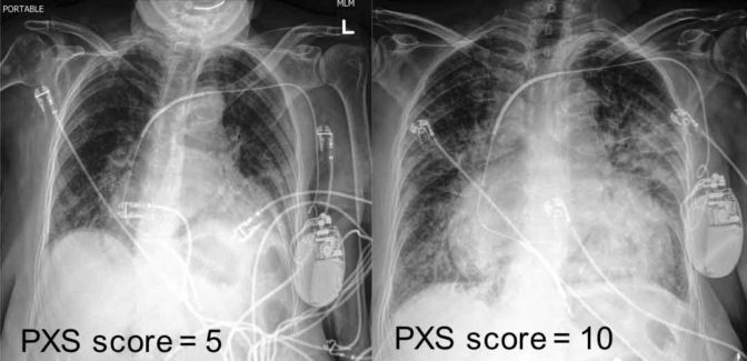
This tool can be used in concert with Li and Kalpathy-Cramer’s research: a risk assessment model that analyzes a chest X-ray to assign a score for lung disease severity. The model can provide clinicians, researchers and infectious disease experts with a consistent, quantitative metric for lung impact, which is described subjectively in typical radiology reports.

Trained on a public dataset of over 150,000 chest X-rays, as well as a few hundred COVID-positive X-rays from Mass General, the severity score AI is being used for testing by four research groups at the hospital using the NVIDIA Clara Deploy SDK. Beyond the pandemic, the team plans to expand the model’s use to more conditions, like pulmonary edema, or wet lung.

Comparing the AI lung disease severity score, or PXS, between images taken at different stages can help clinicians track changes in a patient’s disease over time. (Image from the researchers’ paper in Radiology: Artificial Intelligence, available under open access.)

Foreseeing the Need for Ventilators

Chest imaging is just one variable in a COVID patient’s health. For the broader picture, the Martinos Center team is working with Brandon Westover, executive director of Mass General Brigham’s Clinical Data Animation Center.

Westover is developing AI models that predict clinical outcomes for both admitted patients and outpatient COVID cases, and Kalpathy-Cramer’s lung disease severity score could be integrated as one of the clinical variables for this tool.

The outpatient model analyzes 30 variables to create a risk score for each of hundreds of patients screened at the hospital network’s respiratory infection clinics — predicting the likelihood a patient will end up needing critical care or dying from COVID.

For patients already admitted to the hospital, a neural network predicts the hourly risk that a patient will require artificial breathing support in the next 12 hours, using variables including vital signs, age, pulse oximetry data and respiratory rate.

“These variables can be very subtle, but in combination can provide a pretty strong indication that a patient is getting worse,” Westover said. Running on an NVIDIA Quadro RTX 8000 GPU, the model is accessible through a front-end portal clinicians can use to see who’s most at risk, and which variables are contributing most to the risk score.

Better, Faster, Stronger: Research on NVIDIA DGX

Fischl says NVIDIA DGX systems help Martinos Center researchers more quickly iterate, experimenting with different ways to improve their AI algorithms. DGX A100, with NVIDIA A100 GPUs based on the NVIDIA Ampere architecture, will further speed the team’s work with third-generation Tensor Core technology.

“Quantitative differences make a qualitative difference,” he said. “I can imagine five ways to improve our algorithm, each of which would take seven hours of training. If I can turn those seven hours into just an hour, it makes the development cycle so much more efficient.”

The Martinos Center will use NVIDIA Mellanox switches and VAST Data storage infrastructure, enabling its developers to use NVIDIA GPUDirect technology to bypass the CPU and move data directly into or out of GPU memory, achieving better performance and faster AI training.

“Having access to this high-capacity, high-speed storage will allow us to to analyze raw multimodal data from our research MRI, PET and MEG scanners,” said Matthew Rosen, assistant professor in radiology at Harvard Medical School, who co-directs the Center for Machine Learning at the Martinos Center. “The VAST storage system, when linked with the new A100 GPUs, is going to offer an amazing opportunity to set a new standard for the future of intelligent imaging.”

To learn more about how AI and accelerated computing are helping healthcare institutions fight the pandemic, visit our COVID page.

Main image shows chest x-ray and corresponding heat map, highlighting areas with lung disease. Image from the researchers’ paper in Radiology: Artificial Intelligence, available under open access.

The post Mass General’s Martinos Center Adopts AI for COVID, Radiology Research appeared first on The Official NVIDIA Blog.

Read More

Nerd Watching: GPU-Powered AI Helps Researchers Identify Individual Birds

Nerd Watching: GPU-Powered AI Helps Researchers Identify Individual Birds

Anyone can tell an eagle from an ostrich. It takes a skilled birdwatcher to tell a chipping sparrow from a house sparrow from an American tree sparrow.

Now researchers are using AI to take this to the next level — identifying individual birds.

André Ferreira, a Ph.D. student at France’s Centre for Functional and Evolutionary Ecology, harnessed an NVIDIA GeForce RTX 2070 to train a powerful AI that identifies individual birds within the same species.

It’s the latest example of how deep learning has become a powerful tool for wildlife biologists studying a wide range of animals.

Marine biologists with the U.S. National Oceanic and Atmospheric Research Organization use deep learning to identify and track the endangered North Atlantic Right Whale. Zoologist Dan Rubenstein uses deep learning to distinguish between individuals in herds of Grevy’s Zebras.

The sociable weaver isn’t endangered. But understanding the role of an individual in a group is key to understanding how the birds, native to Southern Africa, work together to build their nests.

The problem: it’s hard to tell the small, rust-colored birds apart, especially when trying to capture their activities in the wild.

In a paper released last week, Ferreira detailed how he and a team of researchers trained a convolutional neural network to identify individual birds.

Ferreira built his model using Keras, a popular open-source neural network library, running on a GeForce RTX 2070 GPU.

He then teamed up with researchers at Germany’s Max Planck Institute of Animal Behavior. Together, they adapted the model to identify wild great tits and captive zebra finches, two other widely studied bird species.

To train their models — a crucial step towards building any modern deep-learning-based AI — researchers made feeders equipped with cameras.

The researchers fitted birds with electronic tags, which triggered sensors in the feeders alerting researchers to the bird’s identity.

This data gave the model a “ground truth” that it could check against for accuracy.

The team’s AI was able to identify individual sociable weavers and wild great tits more than 90 percent of the time. And it identified captive zebra finches 87 percent of the time.

For bird researchers, the work promises several key benefits.

Using cameras and other sensors to track birds allows researchers to study bird behavior much less invasively.

With less need to put researchers in the field, the technique allows researchers to track bird behavior over more extended periods.

Next: Ferreira and his colleagues are working to build AI that can recognize individual birds it has never seen before, and better track groups of birds.

Birdwatching may never be the same.

Featured image credit: Bernard DuPont, some rights reserved.

The post Nerd Watching: GPU-Powered AI Helps Researchers Identify Individual Birds appeared first on The Official NVIDIA Blog.

Read More