The post Introducing the new Facebook Reality Labs, plus save the date for Facebook Connect on September 16 appeared first on Facebook Research.
Rewriting the past: Assessing the field through the lens of language generation
ACL 2020 keynote presentation given by Amazon Scholar and Columbia University professor Kathleen McKeown.Read More

Introducing Danfo.js, a Pandas-like Library in JavaScript
A guest post by Rising Odegua, Independent Researcher; Stephen Oni, Data Science Nigeria
Danfo.js is an open-source JavaScript library that provides high-performance, intuitive, and easy-to-use data structures for manipulating and processing structured data. Danfo.js is heavily inspired by the Python Pandas library and provides a similar interface/API. This means that users familiar with the Pandas API and know JavaScript can easily pick it up.  One of the main goals of Danfo.js is to bring data processing, machine learning and AI tools to JavaScript developers. This is in line with our vision and essentially the vision of the TensorFlow.js team, which is to bring ML to the web. Open-source libraries like Numpy and Pandas revolutionise the ease of manipulating data in Python and lots of tools were built around them, thus driving the bubbling ecosystem of ML in Python.
Danfo.js is built on TensorFlow.js. That is, as Numpy powers Pandas arithmetic operations, we leverage TensorFlow.js to power our low-level arithmetic operations.
Some of the main features of Danfo.js
Danfo.js is fast. It is built on TensorFlow.js, and supports tensors out of the box. This means you can load Tensors in Danfo and also convert Danfo data structure to Tensors. Leveraging these two libraries, you have a data processing library on one hand (Danfo.js), and a powerful ML library on the other hand (TensorFlow.js).
In the example below, we show you how to create a Danfo DataFrame from a tensor object:
const dfd = require("danfojs-node")
const tf = require("@tensorflow/tfjs-node")

let data = tf.tensor2d([[20,30,40], [23,90, 28]])
let df = new dfd.DataFrame(data)
let tf_tensor = df.tensor
console.log(tf_tensor);
tf_tensor.print()
Output:
Tensor {
  kept: false,
  isDisposedInternal: false,
  shape: [ 2, 3 ],
  dtype: 'float32',
  size: 6,
  strides: [ 3 ],
  dataId: {},
  id: 3,
  rankType: '2'
}
Tensor
    [[20, 30, 40],
     [23, 90, 28]]
You can easily convert Arrays, JSONs, or Objects to DataFrame objects for manipulation.
JSON object to DataFrame:
const dfd = require("danfojs-node")
json_data = [{ A: 0.4612, B: 4.28283, C: -1.509, D: -1.1352 },
            { A: 0.5112, B: -0.22863, C: -3.39059, D: 1.1632 },
            { A: 0.6911, B: -0.82863, C: -1.5059, D: 2.1352 },
            { A: 0.4692, B: -1.28863, C: 4.5059, D: 4.1632 }]
df = new dfd.DataFrame(json_data)
df.print()
Output:
Object array with column labels to DataFrame:
const dfd = require("danfojs-node")
obj_data = {'A': [“A1”, “A2”, “A3”, “A4”],
            'B': ["bval1", "bval2", "bval3", "bval4"],
            'C': [10, 20, 30, 40],
            'D': [1.2, 3.45, 60.1, 45],
            'E': ["test", "train", "test", "train"]
            }
df = new dfd.DataFrame(obj_data)
df.print()
Output:
You can easily handle missing data (represented as NaN) in floating point as well as non-floating point data:
const dfd = require("danfojs-node")
let data = {"Name":["Apples", "Mango", "Banana", undefined],
            "Count": [NaN, 5, NaN, 10],
            "Price": [200, 300, 40, 250]}
let df = new dfd.DataFrame(data)
let df_filled = df.fillna({columns: ["Name", "Count"], values: ["Apples",
df["Count"].mean()]})
df_filled.print()
Output: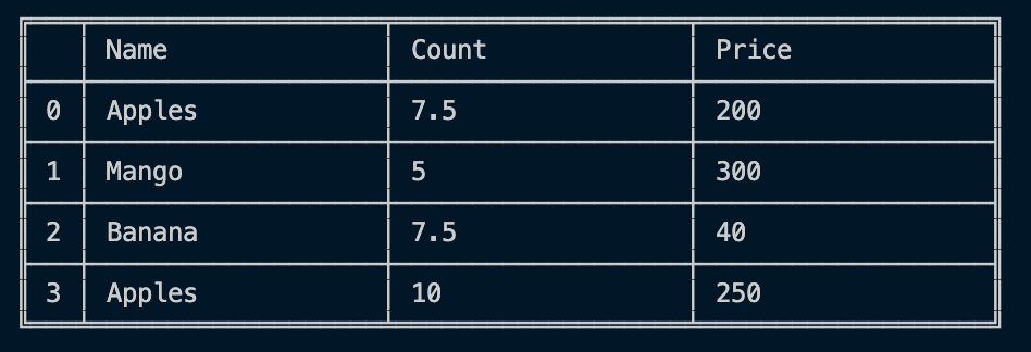
Intelligent label-based slicing, fancy indexing, and querying of large data sets:
const dfd = require("danfojs-node")
let data = { "Name": ["Apples", "Mango", "Banana", "Pear"] ,
            "Count": [21, 5, 30, 10],
             "Price": [200, 300, 40, 250] }

let df = new dfd.DataFrame(data)
let sub_df = df.loc({ rows: ["0:2"], columns: ["Name", "Price"] })
sub_df.print()
Output: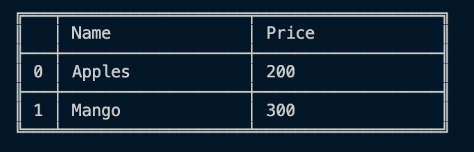
Robust IO tools for loading data from flat-files (CSV and delimited). Both in full and chunks:
const dfd = require("danfojs-node")
//read the first 10000 rows
dfd.read_csv("file:///home/Desktop/bigdata.csv", chunk=10000)
  .then(df => {
    df.tail().print()
  }).catch(err=>{
       console.log(err);
  })
Robust data preprocessing functions like OneHotEncoders, LabelEncoders, and scalers like StandardScaler and MinMaxScaler are supported on DataFrame and Series:
const dfd = require("danfojs-node")
let data = ["dog","cat","man","dog","cat","man","man","cat"]
let series = new dfd.Series(data)
let encode = new dfd.LabelEncoder()
encode.fit(series)
let sf_enc = encode.transform(series)
let new_sf = encode.transform(["dog","man"])
Output: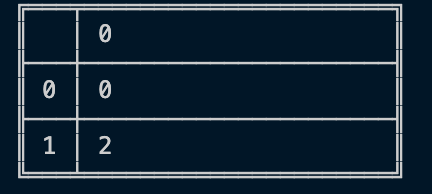
Interactive, flexible and intuitive API for plotting DataFrames and Series in the browser:
<!DOCTYPE html>
<html lang="en">
<head>
    <meta charset="UTF-8">
    <meta name="viewport" content="width=device-width, initial-scale=1.0">
    <script src="https://cdn.jsdelivr.net/npm/danfojs@0.1.1/dist/index.min.js"></script>
    <title>Document</title>
</head>
<body>
    <div id="plot_div"></div>
    <script>
         dfd.read_csv("https://raw.githubusercontent.com/plotly/datasets/master/finance-charts-apple.csv")

            .then(df => {
                var layout = {
                    title: 'A financial charts',
                    xaxis: {title: 'Date'},
                    yaxis: {title: 'Count'}
                }
    new_df = df.set_index({ key: "Date" })
   new_df.plot("plot_div").line({ columns: ["AAPL.Open", "AAPL.High"], layout: layout
})
            }).catch(err => {
                console.log(err);
            })
    </script>
</body>
</html>
Output: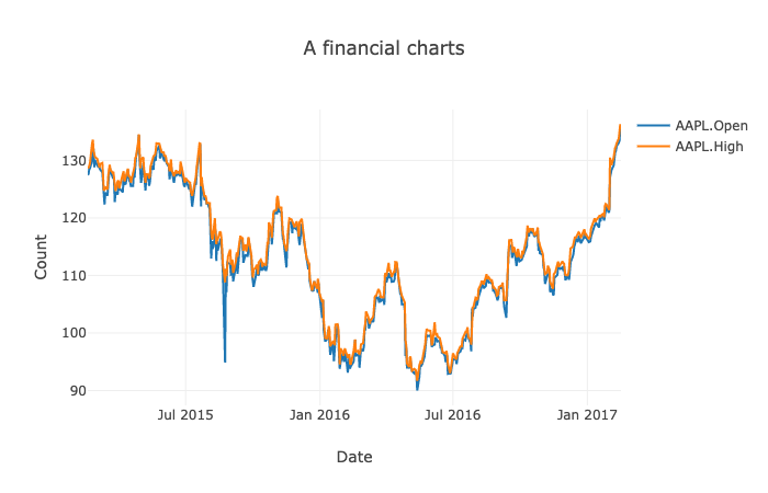
Titanic Survival Prediction using Danfo.js and Tensorflow.js
Below we show a simple end-to-end classification task using Danfo.js and TensorFlow.js. We use Danfo for data loading, manipulating and preprocessing of the dataset, and then export the tensor object.
const dfd = require("danfojs-node")
const tf = require("@tensorflow/tfjs-node")

async function load_process_data() {
    let df = await dfd.read_csv("https://web.stanford.edu/class/archive/cs/cs109/cs109.1166/stuff/titanic.csv")

    //A feature engineering: Extract all titles from names columns
    let title = df['Name'].apply((x) => { return x.split(".")[0] }).values
    //replace in df
    df.addColumn({ column: "Name", value: title })

    //label Encode Name feature
    let encoder = new dfd.LabelEncoder()
    let cols = ["Sex", "Name"]
    cols.forEach(col => {
        encoder.fit(df[col])
        enc_val = encoder.transform(df[col])
        df.addColumn({ column: col, value: enc_val })
    })

    let Xtrain,ytrain;
    Xtrain = df.iloc({ columns: [`1:`] })
    ytrain = df['Survived']

    // Standardize the data with MinMaxScaler
    let scaler = new dfd.MinMaxScaler()
    scaler.fit(Xtrain)
    Xtrain = scaler.transform(Xtrain)

    return [Xtrain.tensor, ytrain.tensor] //return the data as tensors
}
Next, we create a simple neural network using TensorFlow.js.
function get_model() {
    const model = tf.sequential();
    model.add(tf.layers.dense({ inputShape: [7], units: 124, activation: 'relu', kernelInitializer: 'leCunNormal' }));
    model.add(tf.layers.dense({ units: 64, activation: 'relu' }));
    model.add(tf.layers.dense({ units: 32, activation: 'relu' }));
    model.add(tf.layers.dense({ units: 1, activation: "sigmoid" }))
    model.summary();
    return model
}
Finally, we perform training, by first loading the model and the processed data as tensors. This can be fed directly to the neural network.
async function train() {
    const model = await get_model()
    const data = await load_process_data()
    const Xtrain = data[0]
    const ytrain = data[1]

    model.compile({
        optimizer: "rmsprop",
        loss: 'binaryCrossentropy',
        metrics: ['accuracy'],
    });

    console.log("Training started....")
    await model.fit(Xtrain, ytrain,{
        batchSize: 32,
        epochs: 15,
        validationSplit: 0.2,
        callbacks:{
            onEpochEnd: async(epoch, logs)=>{
                console.log(`EPOCH (${epoch + 1}): Train Accuracy: ${(logs.acc * 100).toFixed(2)},
                                                     Val Accuracy:  ${(logs.val_acc * 100).toFixed(2)}n`);
            }
        }
    });
};

train()
The reader will notice that the API of Danfo is very similar to Pandas, and a non-Javascript programmer can easily read and understand the code. You can find the full source code of the demo above here (https://gist.github.com/risenW/f54e4e5b6d92e7b1b9b1f30e884ca83c).
Closing Remarks
As web-based machine learning has matured, it is imperative to have efficient data science tools built specifically for it. Tools like Danfo.js will enable web-based applications to easily support ML features, thus opening the space to an ecosystem of exciting applications. TensorFlow.js started the revolution by providing ML capabilities available in Python, and we hope to see Danfo.js as an efficient partner in this journey. We can’t wait to see what Danfo.js grows into! Hopefully, it becomes indispensable to the web community as well.
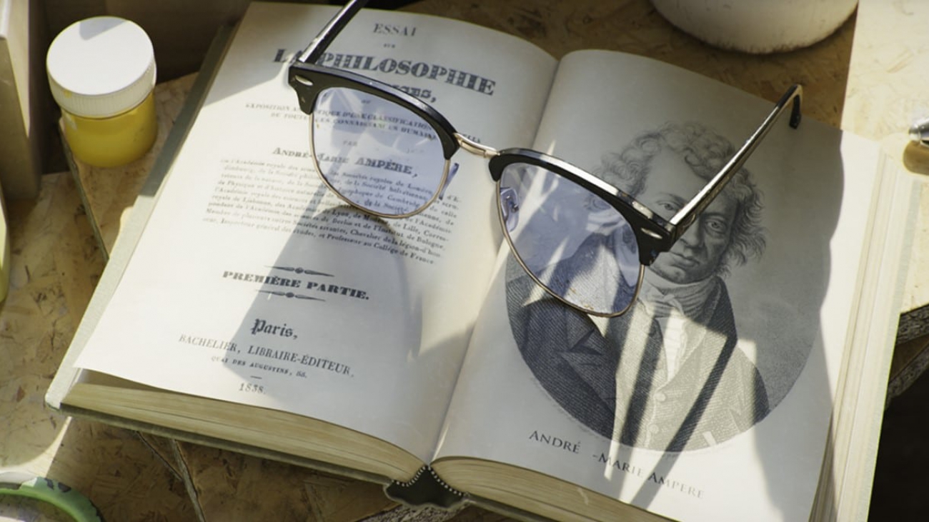
Real-Time Ray Tracing Realized: RTX Brings the Future of Graphics to Millions
Only a dream just a few years ago, real-time ray tracing has become the new reality in graphics because of NVIDIA RTX — and it’s just getting started.
The world’s top gaming franchises, the most popular gaming engines and scores of creative applications across industries are all onboard for real-time ray tracing.
Leading studios, design firms and industry luminaries are using real-time ray tracing to advance content creation and drive new possibilities in graphics, including virtual productions for television, interactive virtual reality experiences, and realistic digital humans and animations.
The Future Group and Riot Games used NVIDIA RTX to deliver the world’s first ray-traced broadcast. Rob Legato, the VFX supervisor for Disney’s recent remake of The Lion King, referred to real-time rendering with GPUs serving as the future of creativity. And developers have adopted real-time techniques to create cinematic video game graphics, like ray-traced reflections in Battlefield V, ray-traced shadows in Shadow of the Tomb Raider and path-traced lighting in Minecraft.
These are just a few of many examples.
In early 2018, ILMxLAB, Epic Games and NVIDIA released a cinematic called Star Wars: Reflections. We revealed that the demo was rendered in real time using ray-traced reflections, area light shadows and ambient occlusion — all on a $70,000 NVIDIA DGX workstation packed with four NVIDIA Volta GPUs. This major advancement captured global attention, as real-time ray tracing with this level of fidelity could only be done offline on gigantic server farms.

Fast forward to August 2018, when we announced the GeForce RTX 2080 Ti at Gamescom and showed Reflections running on just one $1,200 GeForce RTX GPU, with the NVIDIA Turing architecture’s RT Cores accelerating ray tracing performance in real time.
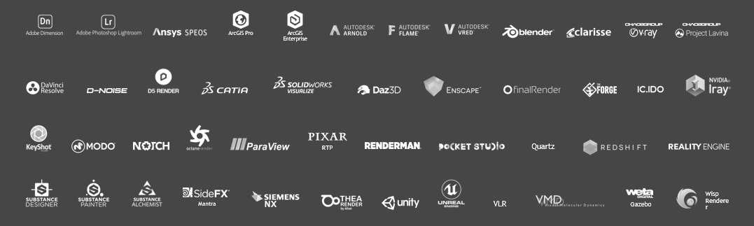
Today, over 50 content creation and design applications, including 20 of the leading commercial renderers, have added support for NVIDIA RTX. Real-time ray tracing is more widely available, allowing professionals to have more time for iterating designs and capturing accurate lighting, shadows, reflections, translucence, scattering and ambient occlusion in their images.
RTX Ray Tracing Continues to Change the Game
From product and building designs to visual effects and animation, real-time ray tracing is revolutionizing content creation. RTX allows creative decisions to be made sooner, as designers no longer need to play the waiting game for renders to complete.

What was once considered impossible just two years ago has now become a reality for anyone with an RTX GPU — NVIDIA’s Turing architecture delivers new capabilities that made real-time ray tracing achievable. Its RT Cores accelerate two of the most computationally intensive tasks: bounding volume hierarchy traversal and ray-triangle intersection testing. This allows the streaming multiprocessors, which perform the computations, to improve programmable shading instead of spending thousands of instruction slots for each ray cast.
Turing’s Tensor Cores enable users to leverage and enhance AI denoising for generating clean images quickly. All of these new features combined are what make real-time ray tracing possible. Creative teams can render images faster, complete more iterations and finish projects with cinematic, photorealistic graphics.
“Ray tracing, especially real-time ray tracing, brings the ground truth to an image and allows the viewer to make immediate, sometimes subconscious decisions about the information,” said Jon Peddie, president of Jon Peddie Research. “If it’s entertainment, the viewer is not distracted and taken out of the story by artifacts and nagging suspension of belief. If it’s engineering, the user knows the results are accurate and can move closer and more quickly to a solution.”

Artists can now use a single GPU for real-time ray tracing to create high-quality imagery, and they can harness the power of RTX through numerous ways. Popular game engines Unity and Unreal Engine are leveraging RTX. GPU renderers like V-Ray, Redshift and Octane are adopting OptiX for RTX acceleration. And workstation vendors like BOXX, Dell, HP, Lenovo and Supermicro offer real-time ray tracing-capable systems, allowing users to harness the power of RTX in a single, flexible desktop or mobile workstation.
RTX GPUs also provide the memory required for handling massive datasets, whether it’s complex geometry or large numbers of high-resolution textures. The NVIDIA Quadro RTX 8000 GPU provides a 48GB frame buffer, and with NVLink high-speed interconnect technology doubling that capacity, users can easily manipulate massive, complex scenes without spending time constantly decimating or optimizing their datasets.
“DNEG’s virtual production department has taken on an ever increasing amount of work, particularly over recent months where practical shoots have become more difficult,” said Stephen Willey, head of technology at DNEG. “NVIDIA’s RTX and Quadro Sync solutions, coupled with Epic’s Unreal Engine, have allowed us to create far larger and more realistic real-time scenes and assets. These advances help us offer exciting new possibilities to our clients.”
More recently, NVIDIA introduced techniques to further improve ray tracing and rendering. With Deep Learning Super Sampling, users can enhance real-time rendering through AI-based super resolution. NVIDIA DLSS allows them to render fewer pixels and use AI to construct sharp, higher-resolution images.
At SIGGRAPH this month, one of our research papers dives deep into how to render dynamic direct lighting and shadows from millions of area lights in real time using a new technique called reservoir-based spatiotemporal importance resampling, or ReSTIR.

Real-Time Ray Tracing Opens New Possibilities for Graphics
RTX ray tracing is transforming design across industries today.
In gaming, the quality of RTX ray tracing creates new dynamics and environments in gameplay, allowing players to use reflective surfaces strategically. For virtual reality, RTX ray tracing brings new levels of realism and immersiveness for professionals in healthcare, AEC and automotive design. And in animation, ray tracing is changing the pipeline completely, enabling artists to easily manage and manipulate light geometry in real time.
Real-time ray tracing is also paving the way for virtual productions and believable digital humans in film, television and immersive experiences like VR and AR.
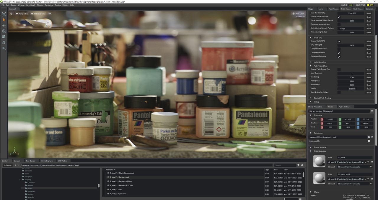
And with NVIDIA Omniverse — the first real-time ray tracer that can scale to any number of GPUs — creatives can simplify collaborative studio workflows with their favorite applications like Unreal Engine, Autodesk Maya and 3ds Max, Substance Painter by Adobe, Unity, SideFX Houdini, and many others. Omniverse is pushing ray tracing forward, enabling users to create visual effects, architectural visualizations and manufacturing designs with dynamic lighting and physically based materials.
Explore the Latest in Ray Tracing and Graphics
Join us at the SIGGRAPH virtual conference to learn more about the latest advances in graphics, and get an exclusive look at some of our most exciting work.
Be part of the NVIDIA community and show us what you can create by participating in our real-time ray tracing contest. The selected winner will receive the latest Quadro RTX graphics card and a free pass to discover what’s new in graphics at NVIDIA GTC, October 5-9.
The post Real-Time Ray Tracing Realized: RTX Brings the Future of Graphics to Millions appeared first on The Official NVIDIA Blog.

AI in Action: NVIDIA Showcases New Research, Enhanced Tools for Creators at SIGGRAPH
The future of graphics is here, and AI is leading the way.
At the SIGGRAPH 2020 virtual conference, NVIDIA is showcasing advanced AI technologies that allow artists to elevate storytelling and create stunning, photorealistic environments like never before.
NVIDIA tools and software are behind the many AI-enhanced features being added to creative tools and applications, powering denoising capabilities, accelerating 8K editing workflows, enhancing material creation and more.
Get an exclusive look at some of our most exciting work, including the new NanoVDB library that boosts workflows for visual effects. And check out our groundbreaking research, AI-powered demos, and speaking sessions to explore the newest possibilities in real-time ray tracing and AI.
NVIDIA Extends OpenVDB with New NanoVDB
OpenVDB is the industry-standard library used by VFX studios for simulating water, fire, smoke, clouds and other effects. As part of its collaborative effort to advance open source software in the motion picture and media industries, the Academy Software Foundation (ASWF) recently announced GPU-acceleration in OpenVDB with the new NanoVDB for faster performance and easier development.
OpenVDB provides a hierarchical data structure and related functions to help with calculating volumetric effects in graphic applications. NanoVDB adds GPU support for the native VDB data structure, which is the foundation for OpenVDB.
With NanoVBD, users can leverage GPUs to accelerate workflows such as ray tracing, filtering and collision detection while maintaining compatibility with OpenVDB. NanoVDB is a bridge between an existing OpenVDB workflow and GPU-accelerated rendering or simulation involving static sparse volumes.

Hear what some partners have been saying about NanoVDB.
“With NanoVDB being added to the upcoming Houdini 18.5 release, we’ve moved the static collisions of our Vellum Solver and the sourcing of our Pyro Solver over to the GPU, giving artists the performance and more fluid experience they crave,” said Jeff Lait, senior mathematician at SideFX.
“ILM has been an early adopter of GPU technology in simulating and rendering dense volumes,” said Dan Bailey, senior software engineer at ILM. “We are excited that the ASWF is going to be the custodian of NanoVDB and now that it offers an efficient sparse volume implementation on the GPU. We can’t wait to try this out in production.”
“After spending just a few days integrating NanoVDB into an unoptimized ray marching prototype of our next generation renderer, it still delivered an order of magnitude improvement on the GPU versus our current CPU-based RenderMan/RIS OpenVDB reference,” said Julian Fong, principal software engineer at Pixar. “We anticipate that NanoVDB will be part of the GPU-acceleration pipeline in our next generation multi-device renderer, RenderMan XPU.”
Learn more about NanoVDB.
Research Takes the Spotlight
During the SIGGRAPH conference, NVIDIA Research and collaborators will share advanced techniques in real-time ray tracing, along with other breakthroughs in graphics and design.
Learn about a new algorithm that allows artists to efficiently render direct lighting from millions of dynamic light sources. Explore a new world of color through nonlinear color triads, which are an extension of gradients that enable artists to enhance image editing and compression.
And hear from leading experts across the industry as they share insights about the future of design:
- Omniverse: Get the latest updates on NVIDIA Omniverse, a computer graphics and simulation platform that lets artists work seamlessly in real time across popular content-creation applications.
- RTX-accelerated ray tracing with OptiX 7: Learn about the general concepts behind OptiX and how to fully optimize your application to get the most out of hardware ray-tracing cores of modern GPUs.
- Making Machine Learning Work: From Ideas to Production Tools: Experts from NVIDIA, Weta Digital, Ubisoft and more will discuss how machine learning is enhancing the production of computer graphics.
- Join a virtual round table with AWS or visit our virtual booth with Microsoft to learn more about Quadro virtual workstations and customer cases.
Check out all the groundbreaking research and presentations from NVIDIA.
Eye-Catching Demos You Can’t Miss
This year at SIGGRAPH, NVIDIA demos will showcase how AI-enhanced tools and GPU-powered simulations are leading a new era of content creation:
- Synthesized high-resolution images with StyleGAN2: Developed by NVIDIA Research, StyleGAN uses transfer learning to produce portraits in a variety of painting styles.
- Mars lander simulation: A high-resolution simulation of retropropulsion is used by NASA scientists to plan how to control the speed and orientation of vehicles under different landing conditions.
- AI denoising on Blender: RTX AI features like OptiX Denoiser enhances rendering to deliver an interactive ray-tracing experience.
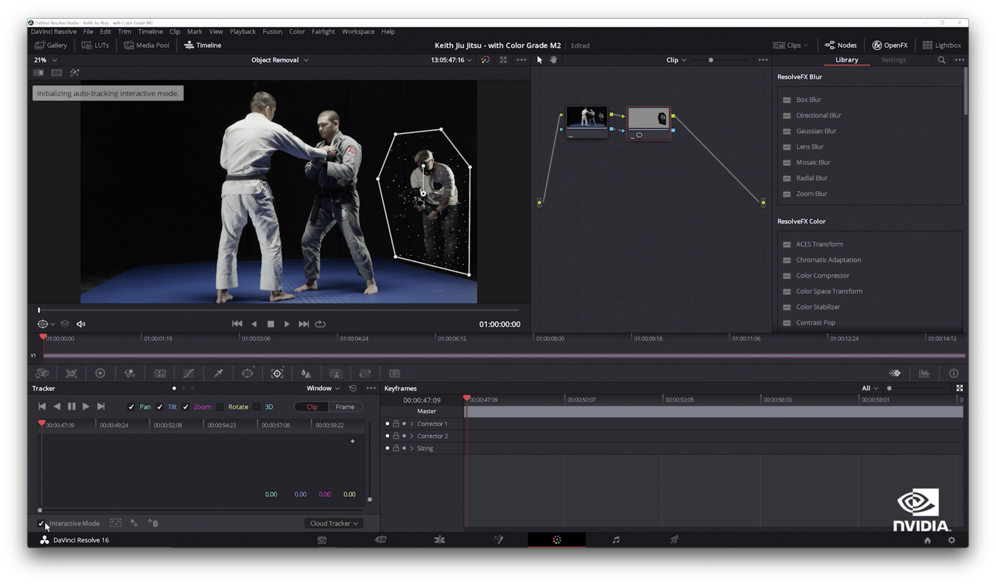
- 8K video editing on RTX Studio laptops: GPU acceleration for advanced video editing and visual effects, including AI-based features in DaVinci Resolve, helping editors produce high-quality video and iterate faster.
Check out all the NVIDIA demos and sessions at SIGGRAPH.
More Exciting Graphics News to Come at GTC
The breakthroughs and innovation doesn’t stop here. Register now to explore more of the latest NVIDIA tools and technologies at GTC, October 5-9.
The post AI in Action: NVIDIA Showcases New Research, Enhanced Tools for Creators at SIGGRAPH appeared first on The Official NVIDIA Blog.
Matthias Bethge: Amazon Scholar and self-proclaimed protopian
His research focuses on how computers can learn the same way as humans.Read More

Introducing TensorFlow Videos for a Global Audience: Japanese
Posted by the TensorFlow Team
When the TensorFlow YouTube channel launched in 2018, we had a vision to inform and inspire developers around the world about what was possible with Machine Learning. With series like Coding TensorFlow showing how you can use it, and Made with TensorFlow showing inspirational stories about what people have done with TensorFlow and much more, the channel has grown greatly. But we learned an important lesson: it’s a global phenomenon, and to reach the world effectively, we should provide content in multiple languages with native speakers presenting. Check out the popular Zero to Hero series in Japanese!
TensorFlow で機械学習ゼロからヒーローへ
最近は、インターネットや新聞、本などを閲覧していると、嫌でも機械学習や AI のようなバズワードが目に入ってくるようになりました。様々な分野で話題になっているおかげで、たくさんの情報が見つかるようになっています。ですが、デベロッパーの視点から見た機械学習とは、一体どういう物なのでしょうか?TensorFlow チームに所属するロレンス・モローニは、その疑問に応えるため、Google I/O 2019 でした好評だったスピーチをベースに、4 部に及ぶ動画シリーズ「機械学習: TensorFlow でゼロからヒーローへ」を作成しました。
第一部では、Java や C++ で作成された具体的なルールに従って動く従来のプログラムと、データからルール自体を推測するシステムである機械学習の違いを学ぶことができます。機械学習とは、どのようなコードで構成されているのか?などの質問に応えるため、シンプルな具体例を使って、機械学習モデルを作成する手順を解説します。ここで語られるいくつかのコンセプトは、第二部の、コンピュータ ビジョンの動画でも応用されています。
第二部では、機械学習を使った基本的なコンピュータ ビジョン(コンピューターに視覚的に確認させ、様々な対象をを認識させること)の仕組みを解説します。こちらのリンク先では、自らコードを実行してみることも可能です : https://goo.gle/34cHkDk
第三部では、なぜ畳み込みニューラル ネットワークがコンピュータ ビジョンの分野で優れているのかを解説します。畳み込みで使われるフィルタに画像を通すと、画像の類似点を明らかにする特徴を捉えてくれます。動画内では、実際に画像にフィルタを適用し、特徴を抽出するプロセスをご覧になっていただけます。
こちらのリンク先では、動画の内容をおさらいすることができます : http://bit.ly/2lGoC5f
第四部では、じゃんけん識別器の作り方を学びます。第一部では、じゃんけんの手を識別するコードを書くことの難しさについて説明しましたが、これまでの 3 つの動画で学んだことを総合し、画像のピクセルからパターンを探し出して、画像を分類し、畳み込みを使って特徴を抽出するニューラル ネットワークを作成するだけで、なんとじゃんけん識別器を自作できてしまいます。
Colab ノート : http://bit.ly/2lXXdw5
データセット : http://bit.ly/2kbV92O
動画シリーズはお楽しみいただけましたでしょうか?もっと知りたいと感じた方は、ぜひフィードバックで教えてください!Read More
Building a customized recommender system in Amazon SageMaker
Recommender systems help you tailor customer experiences on online platforms. Amazon Personalize is an artificial intelligence and machine learning service that specializes in developing recommender system solutions. It automatically examines the data, performs feature and algorithm selection, optimizes the model based on your data, and deploys and hosts the model for real-time recommendation inference. However, if you don’t have explicit user rating data or need to access trained models’ weights, you may need to build your recommender system from scratch. In this post, I show you how to train and deploy a customized recommender system in TensorFlow 2.0, using a Neural Collaborative Filtering (NCF) (He et al., 2017) model on Amazon SageMaker.
Understanding Neural Collaborative Filtering
A recommender system is a set of tools that helps provide users with a personalized experience by predicting user preference amongst a large number of options. Matrix factorization (MF) is a well-known approach to solving such a problem. Conventional MF solutions exploit explicit feedback in a linear fashion; explicit feedback consists of direct user preferences, such as ratings for movies on a five-star scale or binary preference on a product (like or not like). However, explicit feedback isn’t always present in datasets. NCF solves the absence of explicit feedback by only using implicit feedback, which is derived from user activity, such as clicks and views. In addition, NCF utilizes multi-layer perceptron to introduce non-linearity into the solution.
Architecture overview
An NCF model contains two intrinsic sets of network layers: embedding and NCF layers. You use these layers to build a neural matrix factorization solution with two separate network architectures, generalized matrix factorization (GMF) and multi-layer perceptron (MLP), whose outputs are then concatenated as input for the final output layer. The following diagram from the original paper illustrates this architecture.
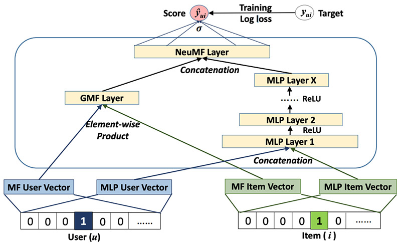
In this post, I walk you through building and deploying the NCF solution using the following steps:
- Prepare data for model training and testing.
- Code the NCF network in TensorFlow 2.0.
- Perform model training using Script Mode and deploy the trained model using Amazon SageMaker hosting services as an endpoint.
- Make a recommendation inference via the model endpoint.
You can find the complete code sample in the GitHub repo.
Preparing the data
For this post, I use the MovieLens dataset. MovieLens is a movie rating dataset provided by GroupLens, a research lab at the University of Minnesota.
First, I run the following code to download the dataset into the ml-latest-small directory:
%%bash
# delete the data directory if it already exists
rm -r ml-latest-small

# download movielens small dataset
curl -O http://files.grouplens.org/datasets/movielens/ml-latest-small.zip

# unzip into data directory
unzip ml-latest-small.zip
rm ml-latest-small.zip
I only use rating.csv, which contains explicit feedback data, as a proxy dataset to demonstrate the NCF solution. To fit this solution to your data, you need to determine the meaning of a user liking an item.
To perform a training and testing split, I take the latest 10 items each user rated as the testing set and keep the rest as the training set:
def train_test_split(df, holdout_num):
    """ perform training testing split

    @param df: dataframe
    @param holdhout_num: number of items to be held out per user as testing items

    @return df_train: training data
    @return df_test testing data

    """
    # first sort the data by time
    df = df.sort_values(['userId', 'timestamp'], ascending=[True, False])

    # perform deep copy to avoid modification on the original dataframe
    df_train = df.copy(deep=True)
    df_test = df.copy(deep=True)

    # get test set
    df_test = df_test.groupby(['userId']).head(holdout_num).reset_index()

    # get train set
    df_train = df_train.merge(
        df_test[['userId', 'movieId']].assign(remove=1),
        how='left'
    ).query('remove != 1').drop('remove', 1).reset_index(drop=True)

    # sanity check to make sure we're not duplicating/losing data
    assert len(df) == len(df_train) + len(df_test)

    return df_train, df_test
Because we’re performing a binary classification task and treating the positive label as if the user liked an item, we need to randomly sample the movies each user hasn’t rated and treat them as negative labels. This is called negative sampling. The following function implements the process:
def negative_sampling(user_ids, movie_ids, items, n_neg):
    """This function creates n_neg negative labels for every positive label

    @param user_ids: list of user ids
    @param movie_ids: list of movie ids
    @param items: unique list of movie ids
    @param n_neg: number of negative labels to sample

    @return df_neg: negative sample dataframe

    """

    neg = []
    ui_pairs = zip(user_ids, movie_ids)
    records = set(ui_pairs)

    # for every positive label case
    for (u, i) in records:
        # generate n_neg negative labels
        for _ in range(n_neg):
            j = np.random.choice(items)
            # resample if the movie already exists for that user
            While (u, j) in records:
                j = np.random.choice(items)
            neg.append([u, j, 0])

    # convert to pandas dataframe for concatenation later
    df_neg = pd.DataFrame(neg, columns=['userId', 'movieId', 'rating'])

    return df_neg
You can use the following code to perform the training and testing splits, negative sampling, and store the processed data in Amazon Simple Storage Service (Amazon S3):
import os
import boto3
import sagemaker
import numpy as np
import pandas as pd

# read rating data
fpath = './ml-latest-small/ratings.csv'
df = pd.read_csv(fpath)

# perform train test split
df_train, df_test = train_test_split(df, 10)

# create 5 negative samples per positive label for training set
neg_train = negative_sampling(
    user_ids=df_train.userId.values,
    movie_ids=df_train.movieId.values,
    items=df.movieId.unique(),
    n_neg=5
)

# create final training and testing sets
df_train = df_train[['userId', 'movieId']].assign(rating=1)
df_train = pd.concat([df_train, neg_train], ignore_index=True)

df_test = df_test[['userId', 'movieId']].assign(rating=1)

# save data locally first
dest = 'ml-latest-small/s3'
!mkdir {dest}
train_path = os.path.join(dest, 'train.npy')
test_path = os.path.join(dest, 'test.npy')
np.save(train_path, df_train.values)
np.save(test_path, df_test.values)

# store data in the default S3 bucket
sagemaker_session = sagemaker.Session()
bucket_name = sm_session.default_bucket()
print("the default bucket name is", bucket_name)

# upload to the default s3 bucket
sagemaker_session.upload_data(train_path, key_prefix='data')
sagemaker_session.upload_data(test_path, key_prefix='data')
I use the Amazon SageMaker session’s default bucket to store processed data. The format of the default bucket name is sagemaker-{region}–{aws-account-id}.
Coding the NCF network
In this section, I implement GMF and MLP separately. These two components’ input are both user and item embeddings. To define the embedding layers, we enter the following code:
def _get_user_embedding_layers(inputs, emb_dim):
    """ create user embeddings """
    user_gmf_emb = tf.keras.layers.Dense(emb_dim, activation='relu')(inputs)
    user_mlp_emb = tf.keras.layers.Dense(emb_dim, activation='relu')(inputs)
    return user_gmf_emb, user_mlp_emb

def _get_item_embedding_layers(inputs, emb_dim):
    """ create item embeddings """
    item_gmf_emb = tf.keras.layers.Dense(emb_dim, activation='relu')(inputs)
    item_mlp_emb = tf.keras.layers.Dense(emb_dim, activation='relu')(inputs)
    return item_gmf_emb, item_mlp_emb
To implement GMF, we multiply the user and item embeddings:
def _gmf(user_emb, item_emb):
    """ general matrix factorization branch """
    gmf_mat = tf.keras.layers.Multiply()([user_emb, item_emb])
    return gmf_mat
The authors of Neural Collaborative Filtering show that a four-layer MLP with 64-dimensional user and item latent factor performed the best across different experiments, so we implement this structure as our MLP:
def _mlp(user_emb, item_emb, dropout_rate):
    """ multi-layer perceptron branch """
    def add_layer(dim, input_layer, dropout_rate):
        hidden_layer = tf.keras.layers.Dense(dim, activation='relu')(input_layer)
        if dropout_rate:
            dropout_layer = tf.keras.layers.Dropout(dropout_rate)(hidden_layer)
            return dropout_layer
        return hidden_layer

    concat_layer = tf.keras.layers.Concatenate()([user_emb, item_emb])
    dropout_l1 = tf.keras.layers.Dropout(dropout_rate)(concat_layer)
    dense_layer_1 = add_layer(64, dropout_l1, dropout_rate)
    dense_layer_2 = add_layer(32, dense_layer_1, dropout_rate)
    dense_layer_3 = add_layer(16, dense_layer_2, None)
    dense_layer_4 = add_layer(8, dense_layer_3, None)
    return dense_layer_4
Lastly, to produce the final prediction, we concatenate the output of GMF and MLP as the following:
def _neuCF(gmf, mlp, dropout_rate):
    """ final output layer """
    concat_layer = tf.keras.layers.Concatenate()([gmf, mlp])
    output_layer = tf.keras.layers.Dense(1, activation='sigmoid')(concat_layer)
    return output_layer
To build the entire solution in one step, we create a graph building function:
def build_graph(user_dim, item_dim, dropout_rate=0.25):
    """ neural collaborative filtering model

    @param user_dim: one hot encoded user dimension
    @param item_dim: one hot encoded item dimension
    @param dropout_rate: drop out rate for dropout layers

    @return model: neural collaborative filtering model graph

    """

    user_input = tf.keras.Input(shape=(user_dim))
    item_input = tf.keras.Input(shape=(item_dim))

    # create embedding layers
    user_gmf_emb, user_mlp_emb = _get_user_embedding_layers(user_input, 32)
    item_gmf_emb, item_mlp_emb = _get_item_embedding_layers(item_input, 32)

    # general matrix factorization
    gmf = _gmf(user_gmf_emb, item_gmf_emb)

    # multi layer perceptron
    mlp = _mlp(user_mlp_emb, item_mlp_emb, dropout_rate)

    # output
    output = _neuCF(gmf, mlp, dropout_rate)

    # create the model
    model = tf.keras.Model(inputs=[user_input, item_input], outputs=output)

    return model
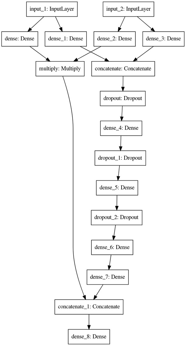
I use the Keras plot_model utility to verify the network architecture I just built is correct:
# build graph
ncf_model = build_graph(n_user, n_item)

# visualize and save to a local png file
tf.keras.utils.plot_model(ncf_model, to_file="neural_collaborative_filtering_model.png")
The output architecture should look like the following diagram.
Training and deploying the model
For instructions on deploying a model you trained using an instance on Amazon SageMaker, see Deploy trained Keras or TensorFlow models using Amazon SageMaker. For this post, I deploy this model using Script Mode.
We first need to create a Python script that contains the model training code. I compiled the model architecture code presented previously and added additional code required in the ncf.py, which you can use directly. I also implemented a function for you to load training data; to load testing data, the function is the same except the file name is changed to reflect the testing data destination. See the following code:
def _load_training_data(base_dir):
    """ load training data """
    df_train = np.load(os.path.join(base_dir, 'train.npy'))
    user_train, item_train, y_train = np.split(np.transpose(df_train).flatten(), 3)
    return user_train, item_train, y_train
After downloading the training script and storing it in the same directory as the model training notebook, we can initialize a TensorFlow estimator with the following code:
ncf_estimator = TensorFlow(
    entry_point='ncf.py',
    role=role,
    train_instance_count=1,
    train_instance_type='ml.c5.2xlarge',
    framework_version='2.1.0',
    py_version='py3',
    distributions={'parameter_server': {'enabled': True}},
    hyperparameters={'epochs': 3, 'batch_size': 256, 'n_user': n_user, 'n_item': n_item}
)
We fit the estimator to our training data to start the training job:
# specify the location of the training data
training_data_uri = os.path.join(f's3://{bucket_name}', 'data')
# kick off the training job
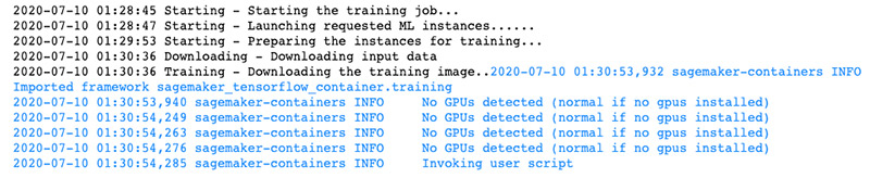
ncf_estimator.fit(training_data_uri)
When you see the output in the following screenshot, your model training job has started.
When the model training process is complete, we can deploy the model as an endpoint. See the following code:
predictor = ncf_estimator.deploy(initial_instance_count=1,
                                 instance_type='ml.c5.xlarge',
                                 endpoint_type='tensorflow-serving')
Performing model inference
To make inference using the endpoint on the testing set, we can invoke the model in the same way by using TensorFlow Serving:
# Define a function to read testing data
def _load_testing_data(base_dir):
    """ load testing data """
    df_test = np.load(os.path.join(base_dir, 'test.npy'))
    user_test, item_test, y_test = np.split(np.transpose(df_test).flatten(), 3)
    return user_test, item_test, y_test

# read testing data from local
user_test, item_test, test_labels = _load_testing_data('./ml-latest-small/s3/')

# one-hot encode the testing data for model input
with tf.Session() as tf_sess:
    test_user_data = tf_sess.run(tf.one_hot(user_test, depth=n_user)).tolist()
    test_item_data = tf_sess.run(tf.one_hot(item_test, depth=n_item)).tolist()

# make batch prediction
batch_size = 100
y_pred = []
for idx in range(0, len(test_user_data), batch_size):
    # reformat test samples into tensorflow serving acceptable format
    input_vals = {
     "instances": [
         {'input_1': u, 'input_2': i}
         for (u, i) in zip(test_user_data[idx:idx+batch_size], test_item_data[idx:idx+batch_size])
    ]}

    # invoke model endpoint to make inference
    pred = predictor.predict(input_vals)

    # store predictions
    y_pred.extend([i[0] for i in pred['predictions']])
The model output is a set of probabilities, ranging from 0 to 1, for each user-item pair that we specify for inference. To make final binary predictions, such as like or not like, we need to apply a threshold. For demonstration purposes, I use 0.5 as a threshold; if the predicted probability is equal or greater than 0.5, we say the model predicts the user will like the item, and vice versa.
# combine user id, movie id, and prediction in one dataframe
pred_df = pd.DataFrame([
user_test,
item_test,
(np.array(y_pred) >= 0.5).astype(int)],
).T
# assign column names to the dataframe
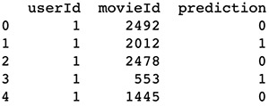
pred_df.columns = ['userId', 'movieId', 'prediction']
Finally, we can get a list of model predictions on whether a user will like a movie, as shown in the following screenshot.
Conclusion
Designing a recommender system can be a challenging task that sometimes requires model customization. In this post, I showed you how to implement, deploy, and invoke an NCF model from scratch in Amazon SageMaker. This work can serve as a foundation for you to start building more customized solutions with your own datasets.
For more information about using built-in Amazon SageMaker algorithms and Amazon Personalize to build recommender system solutions, see the following:
- Omnichannel personalization with Amazon Personalize
- Creating a recommendation engine using Amazon Personalize
- Extending Amazon SageMaker factorization machines algorithms to predict top x recommendations
- Build a movie recommender with factorization machines on Amazon SageMaker
To further customize the Neural Collaborative Filtering network, Deep Matrix Factorization (Xue et al., 2017) model can be an option. For more information, see Build a Recommendation Engine on AWS Today.
About the Author
 Taihua (Ray) Li is a data scientist with AWS Professional Services. He holds a M.S. in Predictive Analytics degree from DePaul University and has several years of experience building artificial intelligence powered applications for non-profit and enterprise organizations. At AWS, Ray helps customers to unlock business potentials and to drive actionable outcomes with machine learning. Outside of work, he enjoys fitness classes, biking, and traveling.
Announcing the winners of the Economic Impact of Digital Technologies request for proposals
In January 2020, Facebook announced a $1 million commitment in 2020 to fund projects measuring the impact of social media and digital technologies on the economy as well as on economic opportunity. The first round of grant awards, announced in early June, was focused broadly on the economic impact of digital tools for small- and medium-sized businesses.
As a continuation of this series, we announced the Economic Impact of Digital Technologies request for proposals in April 2020. Today, we are announcing the winners of this second round of research awards.
During our review of these proposals, the importance of this work has become all the more evident. The ongoing effects of the COVID-19 pandemic throughout the globe is leading many small- and medium-sized businesses to operate online as a way to adapt. To better understand these challenges and opportunities, our winning proposals reflect compelling work on myriad technologies being used by these businesses, examining pertinent topics such as digital ads, marketing, payments, and other touchstones of digital technologies.
We received 189 proposals from 39 countries. Winning proposals span research agendas, from examining ad strategies used by minority-owned businesses to reach consumers, to small businesses’ use of contactless payments. We believe these proposals will help paint a picture of economic recovery across sectors for these businesses.
Thank you to all the researchers who took the time to submit a proposal, and congratulations to the award recipients. We are excited about the insights these researchers will contribute, as well as the rigor and thoughtfulness with which they will advance our knowledge of how to help small businesses.
For more information about areas of interest, eligibility, requirements, and more, visit the application page.
Research award winners
Principal investigators are listed first unless otherwise noted.
Digital sales and inventory technology to assess SMBs’ creditworthiness
Sean Higgins (Northwestern University), Paul Gertler (University of California, Berkeley), Ulrike Malmendier (University of California, Berkeley), and Waldo Ojeda (City University of New York)
The impact of social media marketing on business growth in times of crisis
Laura Zimmermann (IE University), Naufel J. Vilcassin (London School of Economics), Pradeep K. Chintagunta (University of Chicago), and Stephen J. Anderson (University of Texas at Austin)
Impact of contactless payments for small business services
Sophia T. Anong and Joan Koonce (University of Georgia)
Comparing data-driven with contextual advertising for small restaurants
Xi Y. Leung and Jiyoung Kim (University of North Texas)
Business agility — the critical role of data-driven and digital advertising
Eko Agus Prasetio, Ayu Purwariyanti, Dedy Sushandoyo, Muhammad Irham Rahadhian, Naufal Al Labib Tisyadi, and Retna Ayu Mustikarini Kencanasari (Bandung Institute of Technology)
The post Announcing the winners of the Economic Impact of Digital Technologies request for proposals appeared first on Facebook Research.
Google at ECCV 2020
This week, the 16th European Conference on Computer Vision (ECCV2020) begins, a premier forum for the dissemination of research in computer vision and related fields. Being held virtually for the first time this year, Google is proud to be an ECCV2020 Platinum Partner and is excited to share our research with the community with nearly 50 accepted publications, alongside several tutorials and workshops.
If you are registered for ECCV this year, please visit our virtual booth in the Platinum Exhibition Hall to learn more about the research we’re presenting at ECCV 2020, including some demos and opportunities to connect with our researchers. You can also learn more about our contributions below (Google affiliations in bold).
Organizing Committee
General Chairs: Vittorio Ferrari, Bob Fisher, Cordelia Schmid, Emanuele TrucoAcademic Demonstrations Chair: Thomas Mensink
Accepted Publications
NeRF: Representing Scenes as Neural Radiance Fields for View Synthesis (Honorable Mention Award)
Ben Mildenhall, Pratul Srinivasan, Matthew Tancik, Jonathan T. Barron, Ravi Ramamoorthi, Ren Ng
Quaternion Equivariant Capsule Networks for 3D Point Clouds
Yongheng Zhao, Tolga Birdal, Jan Eric Lenssen, Emanuele Menegatti, Leonidas Guibas, Federico Tombari
SoftpoolNet: Shape Descriptor for Point Cloud Completion and Classification
Yida Wang, David Joseph Tan, Nassir Navab, Federico Tombari
Combining Implicit Function Learning and Parametric Models for 3D Human Reconstruction
Bharat Lal Bhatnagar, Cristian Sminchisescu, Christian Theobalt, Gerard Pons-Moll
CoReNet: Coherent 3D scene reconstruction from a single RGB image
Stefan Popov, Pablo Bauszat, Vittorio Ferrari
Adversarial Generative Grammars for Human Activity Prediction
AJ Piergiovanni, Anelia Angelova, Alexander Toshev, Michael S. Ryoo
Self6D: Self-Supervised Monocular 6D Object Pose Estimation
Gu Wang, Fabian Manhardt, Jianzhun Shao, Xiangyang Ji, Nassir Navab, Federico Tombari
Du2Net: Learning Depth Estimation from Dual-Cameras and Dual-Pixels
Yinda Zhang, Neal Wadhwa, Sergio Orts-Escolano, Christian Häne, Sean Fanello, Rahul Garg
What Matters in Unsupervised Optical Flow
Rico Jonschkowski, Austin Stone, Jonathan T. Barron, Ariel Gordon, Kurt Konolige, Anelia Angelova
Appearance Consensus Driven Self-Supervised Human Mesh Recovery
Jogendra N. Kundu, Mugalodi Rakesh, Varun Jampani, Rahul M. Venkatesh, R. Venkatesh Babu
Fashionpedia: Ontology, Segmentation, and an Attribute Localization Dataset
Menglin Jia, Mengyun Shi, Mikhail Sirotenko, Yin Cui, Claire Cardie, Bharath Hariharan, Hartwig Adam, Serge Belongie
PointMixup: Augmentation for Point Clouds
Yunlu Chen, Vincent Tao Hu, Efstratios Gavves, Thomas Mensink, Pascal Mettes1, Pengwan Yang, Cees Snoek
Connecting Vision and Language with Localized Narratives (see our blog post)
Jordi Pont-Tuset, Jasper Uijlings, Soravit Changpinyo, Radu Soricut, Vittorio Ferrari
Big Transfer (BiT): General Visual Representation Learning (see our blog post)
Alexander Kolesnikov, Lucas Beyer, Xiaohua Zhai, Joan Puigcerver, Jessica Yung, Sylvain Gelly, Neil Houlsby
View-Invariant Probabilistic Embedding for Human Pose
Jennifer J. Sun, Jiaping Zhao, Liang-Chieh Chen, Florian Schroff, Hartwig Adam, Ting Liu
Axial-DeepLab: Stand-Alone Axial-Attention for Panoptic Segmentation
Huiyu Wang, Yukun Zhu, Bradley Green, Hartwig Adam, Alan Yuille, Liang-Chieh Chen
Mask2CAD: 3D Shape Prediction by Learning to Segment and Retrieve
Weicheng Kuo, Anelia Angelova, Tsung-Yi Lin, Angela Dai
A Generalization of Otsu’s Method and Minimum Error Thresholding
Jonathan T. Barron
Learning to Factorize and Relight a City
Andrew Liu, Shiry Ginosar, Tinghui Zhou, Alexei A. Efros, Noah Snavely
Weakly Supervised 3D Human Pose and Shape Reconstruction with Normalizing Flows
Andrei Zanfir, Eduard Gabriel Bazavan, Hongyi Xu, Bill Freeman, Rahul Sukthankar, Cristian Sminchisescu
Multi-modal Transformer for Video Retrieval
Valentin Gabeur, Chen Sun, Karteek Alahari, Cordelia Schmid
Generative Latent Textured Proxies for Category-Level Object Modeling
Ricardo Martin Brualla, Sofien Bouaziz, Matthew Brown, Rohit Pandey, Dan B Goldman
Neural Design Network: Graphic Layout Generation with Constraints
Hsin-Ying Lee*, Lu Jiang, Irfan Essa, Phuong B Le, Haifeng Gong, Ming-Hsuan Yang, Weilong Yang
Neural Articulated Shape Approximation
Boyang Deng, Gerard Pons-Moll, Timothy Jeruzalski, JP Lewis, Geoffrey Hinton, Mohammad Norouzi, Andrea Tagliasacchi
Uncertainty-Aware Weakly Supervised Action Detection from Untrimmed Videos
Anurag Arnab, Arsha Nagrani, Chen Sun, Cordelia Schmid
Beyond Controlled Environments: 3D Camera Re-Localization in Changing Indoor Scenes
Johanna Wald, Torsten Sattler, Stuart Golodetz, Tommaso Cavallari, Federico Tombari
Consistency Guided Scene Flow Estimation
Yuhua Chen, Luc Van Gool, Cordelia Schmid, Cristian Sminchisescu
Continuous Adaptation for Interactive Object Segmentation by Learning from Corrections
Theodora Kontogianni*, Michael Gygli, Jasper Uijlings, Vittorio Ferrari
SimPose: Effectively Learning DensePose and Surface Normal of People from Simulated Data
Tyler Lixuan Zhu, Per Karlsson, Christoph Bregler
Learning Data Augmentation Strategies for Object Detection
Barret Zoph, Ekin Dogus Cubuk, Golnaz Ghiasi, Tsung-Yi Lin, Jonathon Shlens, Quoc V Le
Streaming Object Detection for 3-D Point Clouds
Wei Han, Zhengdong Zhang, Benjamin Caine, Brandon Yang, Christoph Sprunk, Ouais Alsharif, Jiquan Ngiam, Vijay Vasudevan, Jonathon Shlens, Zhifeng Chen
Improving 3D Object Detection through Progressive Population Based Augmentation
Shuyang Cheng, Zhaoqi Leng, Ekin Dogus Cubuk, Barret Zoph, Chunyan Bai, Jiquan Ngiam, Yang Song, Benjamin Caine, Vijay Vasudevan, Congcong Li, Quoc V. Le, Jonathon Shlens, Dragomir Anguelov
An LSTM Approach to Temporal 3D Object Detection in LiDAR Point Clouds
Rui Huang, Wanyue Zhang, Abhijit Kundu, Caroline Pantofaru, David A Ross, Thomas Funkhouser, Alireza Fathi
BigNAS: Scaling Up Neural Architecture Search with Big Single-Stage Models
Jiahui Yu, Pengchong Jin, Hanxiao Liu, Gabriel Bender, Pieter-Jan Kindermans, Mingxing Tan, Thomas Huang, Xiaodan Song, Ruoming Pang, Quoc Le
Memory-Efficient Incremental Learning Through Feature Adaptation
Ahmet Iscen, Jeffrey Zhang, Svetlana Lazebnik, Cordelia Schmid
Virtual Multi-view Fusion for 3D Semantic Segmentation
Abhijit Kundu, Xiaoqi Yin, Alireza Fathi, David A Ross, Brian E Brewington, Thomas Funkhouser, Caroline Pantofaru
Efficient Scale-permuted Backbone with Learned Resource Distribution
Xianzhi Du, Tsung-Yi Lin, Pengchong Jin, Yin Cui, Mingxing Tan, Quoc V Le, Xiaodan Song
RetrieveGAN: Image Synthesis via Differentiable Patch Retrieval
Hung-Yu Tseng*, Hsin-Ying Lee*, Lu Jiang, Ming-Hsuan Yang, Weilong Yang
Graph convolutional networks for learning with few clean and many noisy labels
Ahmet Iscen, Giorgos Tolias, Yannis Avrithis, Ondrej Chum, Cordelia Schmid
Deep Positional and Relational Feature Learning for Rotation-Invariant Point Cloud Analysis
Ruixuan Yu, Xin Wei, Federico Tombari, Jian Sun
Federated Visual Classification with Real-World Data Distribution
Tzu-Ming Harry Hsu, Hang Qi, Matthew Brown
Joint Bilateral Learning for Real-time Universal Photorealistic Style Transfer
Xide Xia, Meng Zhang, Tianfan Xue, Zheng Sun, Hui Fang, Brian Kulis, Jiawen Chen
AssembleNet++: Assembling Modality Representations via Attention Connections
Michael S. Ryoo, AJ Piergiovanni, Juhana Kangaspunta, Anelia Angelova
Naive-Student: Leveraging Semi-Supervised Learning in Video Sequences for Urban Scene Segmentation
Liang-Chieh Chen, Raphael Gontijo-Lopes, Bowen Cheng, Maxwell D. Collins, Ekin D. Cubuk, Barret Zoph, Hartwig Adam, Jonathon Shlens
AttentionNAS: Spatiotemporal Attention Cell Search for Video Classification
Xiaofang Wang, Xuehan Xiong, Maxim Neumann, AJ Piergiovanni, Michael S. Ryoo, Anelia Angelova, Kris M. Kitani, Wei Hua
Unifying Deep Local and Global Features for Image Search
Bingyi Cao, Andre Araujo, Jack Sim
Pillar-based Object Detection for Autonomous Driving
Yue Wang, Alireza Fathi, Abhijit Kundu, David Ross, Caroline Pantofaru, Tom Funkhouser, Justin Solomon
Improving Object Detection with Selective Self-supervised Self-training
Yandong Li, Di Huang, Danfeng Qin, Liqiang Wang, Boqing Gong
Environment-agnostic Multitask Learning for Natural Language Grounded NavigationXin Eric Wang*, Vihan Jain, Eugene Ie, William Yang Wang, Zornitsa Kozareva, Sujith Ravi
SimAug: Learning Robust Representations from Simulation for Trajectory Prediction
Junwei Liang, Lu Jiang, Alex Hauptmann
Tutorials
New Frontiers for Learning with Limited Labels or Data
Organizers: Shalini De Mello, Sifei Liu, Zhiding Yu, Pavlo Molchanov, Varun Jampani, Arash Vahdat, Animashree Anandkumar, Jan Kautz
Weakly Supervised Learning in Computer Vision
Organizers: Seong Joon Oh, Rodrigo Benenson, Hakan Bilen
Workshops
Joint COCO and LVIS Recognition Challenge
Organizers: Alexander Kirillov, Tsung-Yi Lin, Yin Cui, Matteo Ruggero Ronchi, Agrim Gupta, Ross Girshick, Piotr Dollar
4D Vision
Organizers: Anelia Angelova, Vincent Casser, Jürgen Sturm, Noah Snavely, Rahul Sukthankar
GigaVision: When Gigapixel Videography Meets Computer Vision
Organizers: Lu Fang, Shengjin Wang, David J. Brady, Feng Yang
Advances in Image Manipulation Workshop and Challenges
Organizers: Radu Timofte, Andrey Ignatov, Luc Van Gool, Wangmeng Zuo, Ming-Hsuan Yang, Kyoung Mu Lee, Liang Lin, Eli Shechtman, Kai Zhang, Dario Fuoli, Zhiwu Huang, Martin Danelljan, Shuhang Gu, Ming-Yu Liu, Seungjun Nah, Sanghyun Son, Jaerin Lee, Andres Romero, ETH Zurich, Hannan Lu, Ruofan Zhou, Majed El Helou, Sabine Süsstrunk, Roey Mechrez, BeyondMinds & Technion, Pengxu Wei, Evangelos Ntavelis, Siavash Bigdeli
Robust Vision Challenge 2020
Organizers:Oliver Zendel, Hassan Abu Alhaija, Rodrigo Benenson, Marius Cordts, Angela Dai, Xavier Puig Fernandez, Andreas Geiger, Niklas Hanselmann, Nicolas Jourdan, Vladlen Koltun, Peter Kontschider, Alina Kuznetsova, Yubin Kang, Tsung-Yi Lin, Claudio Michaelis, Gerhard Neuhold, Matthias Niessner, Marc Pollefeys, Rene Ranftl, Carsten Rother, Torsten Sattler, Daniel Scharstein, Hendrik Schilling, Nick Schneider, Jonas Uhrig, Xiu-Shen Wei, Jonas Wulff, Bolei Zhou
“Deep Internal Learning”: Training with no prior examples
Organizers: Michal Irani,Tomer Michaeli, Tali Dekel, Assaf Shocher, Tamar Rott Shaham
Instance-Level Recognition
Organizers: Andre Araujo, Cam Askew, Bingyi Cao, Ondrej Chum, Bohyung Han, Torsten Sattler, Jack Sim, Giorgos Tolias, Tobias Weyand, Xu Zhang
Women in Computer Vision Workshop (WiCV) (Platinum Sponsor)
Panel Participation: Dina Damen, Sanja Fiddler, Zeynep Akata, Grady Booch, Rahul Sukthankar
*Work performed while at Google
