Selecting the right metadata to build high-performing recommendation models with Amazon Personalize

Selecting the right metadata to build high-performing recommendation models with Amazon Personalize

In this post, we show you how to select the right metadata for your use case when building a recommendation engine using Amazon Personalize. The aim is to help you optimize your models to generate more user-relevant recommendations. We look at which metadata is most relevant to include for different use cases, and where you may get better results by excluding other metadata. We also highlight a specific use case from Pulselive, one of our customers that recently used Amazon Personalize to enhance the recommendation capabilities of their customer’s websites, resulting in a 20% increase in video consumption.

Introducing Amazon Personalize

Amazon Personalize is a managed service that enables you to improve customer engagement by powering personalized product and content recommendations, and targeted marketing promotions. Amazon Personalize uses machine learning (ML) to create high-quality recommendations that you can use to personalize your user experience across digital channels such as websites, applications, and email systems. You can get started without any prior ML experience using simple APIs to easily build sophisticated personalization capabilities in just a few clicks. Amazon Personalize automatically processes and examines your metadata, identifies what is meaningful, allows you to pick an ML algorithm, and trains and optimizes a custom model based on your metadata. All your data is encrypted to be private and secure, and is only used to create recommendations for your users.

Let’s dive into how important that metadata is to get a performant model.

The role metadata selection plays in recommendations

The goal of metadata selection in recommendation engines is to select the right data to aid the training algorithm to discover valuable information about the similarities in user preferences and behavior, in addition to the properties and similarity of the items you’re trying to recommend through the engine. The ultimate goal is to provide a personalized experience, uniquely tailored for each user, and present them with the items that are the most relevant to them.

Nowadays, there are so many sources of data that a company could potentially use to capture user behavior and understand which items to present to them that it has become challenging to accurately select which metadata to consider and which to ignore. Irrespective of the use case, a commercial website can use large amounts of data about every aspect of each user’s behavior on the website, such as which items they’re frequently interacting with (watching a video or ordering an item), how long they spend on each item’s page, or even how erratic or smooth the movement of their cursor is while scrolling through a page. All this information can reveal a lot about a user’s preferences and what would be the ideal items to recommend to them.

There are two main categories of approaches to recommendation engines: collaborative filtering and content-based filtering.

Collaborative filtering compares the behavior of the users with each other and tries to calculate the similarity between them to find shared interests. Therefore, the recommendation engine knows that if user A has very similar behavior to user B, then user A would likely be interested in some of the items that user B has interacted with, and vice versa.

Content-based filtering looks at the actual items the users interact with. If a user has interacted with items A and B, and product C is very similar to A and B, then item C will likely be of interest to the user.

We also have hybrid models that use both user behavior and item-related data to find the underlying patterns that reveal the ideal items to recommend to each user.

Each method requires a different approach to metadata selection because they require different types of data to be collected and used for the training. For example, building collaborative filtering engines requires data related to the behavior of users on the website, whereas building a content-based engine requires more data related to the items (item-specific metadata and which users interacted with which items). A hybrid solution requires data related to both the users and the items.

As a general rule, authenticated experiences are most optimal. When your users have personal accounts that they log in to, you can provide them with a more personalized experience tailored to their needs because you can easily track and record every aspect of their behavior (along with additional metadata), whereas it’s harder to track anonymous or guest users and map them to their previous sessions.

The problems that can occur if metadata selection isn’t done right

If metadata selection isn’t done correctly, it can potentially lead to poor recommendations that are either too generic (showing most users the most popular and commonly interacted products) or not relevant (showing items that are completely irrelevant to the unique user).

When too much information is included in training a recommendation model, it can lead to noise in the model. Metadata that has no correlation with user preferences but was included in training skews the model and makes it harder for the algorithm to find the valuable underlying patterns that allow for a successful recommender system.

This can also apply to the depth (amount of history) of the data that is used to train a model. Perhaps relevant metadata has been selected, but the freshness of the data in many cases is a stronger indicator of relevance—the most recent metadata is more relevant than historical data for the same kind of interactions. This is because user behavior and preferences vary over time and people’s interests can change rather quickly; therefore, presenting a user with a recommendation that was considered relevant to them a few months ago doesn’t guarantee that the recommendation is relevant to them today. This is why it’s important to keep your recommender system up to date with current user behavior.

Conversely, if too little information is included, the recommendation model under-performs. If you don’t include valuable information that can aid the performance of the model, the recommendation model makes suboptimal suggestions.

A wrong approach to metadata selection can make it harder for the algorithms to find the underlying patterns that connect users and items. This means that the recommendations that the users are presented with aren’t personalized as expected.

Terminology of recommendation engines

To introduce the topic further, let’s dive into some of the terminology associated with Amazon Personalize:

  • Datasets and dataset groupsDatasets contain the data used to train a recommendation model. You can use different dataset groups to serve different purposes. For example, separate applications, with their own users and items, can have their own dataset groups.
  • Recipes and solutions – Amazon Personalize uses recipes, which are the combination of the learning algorithm with the hyperparameters and datasets used. Training a model with different recipes leads to different results. The resultant models that are deployed are referred to as a solution version.
  • Campaigns – A deployed solution version is known as a campaign. A campaign allows Amazon Personalize to make recommendations for your users.

Metadata types are dictated in the datasets used to train a model. In the following section, we look at how to do that.

Selecting metadata

Amazon Personalize uses different recipes that are aimed towards either of the two main categories of recommendation engines—collaborative filtering and content-based filtering—and also the hybrid methods. For more information about pre-defined recipes, see Choosing a Recipe.

No matter which recipe you chose to work with, Amazon Personalize has three main types of datasets that it can use to build models (solutions), and each is related to one of the following categories:

  • Users
  • Items
  • Interactions

The users and items dataset types are known as metadata types, and are only used by certain recipes. As their names imply, their metadata has unique fields that describe each individual user or item. User metadata could be age, gender, and geography. Typical item metadata is color, category, shape, price (in the case of items) or content category, ratings, and genre, if the type of item we’re trying to recommend is a video or movie.

The interactions metadata is the direct interactions of a user with an item, which is usually the most revealing information for the relationship between users and items. Some examples of interactions data can be clicks (user A clicked on item X), purchases (user actually purchased an item), amount of time spent on an item’s webpage, the addition of an item to a user’s wishlist, or even the fact that the user hovered their cursor for a few milliseconds more than usual over a certain item.

The minimum number of interactions Amazon Personalize expects in order to start making recommendations is 1,000 interactions from a minimum of 25 users. User and item metadata datasets are optional, and their importance depends on your use case and the algorithm (recipe) you’re using.

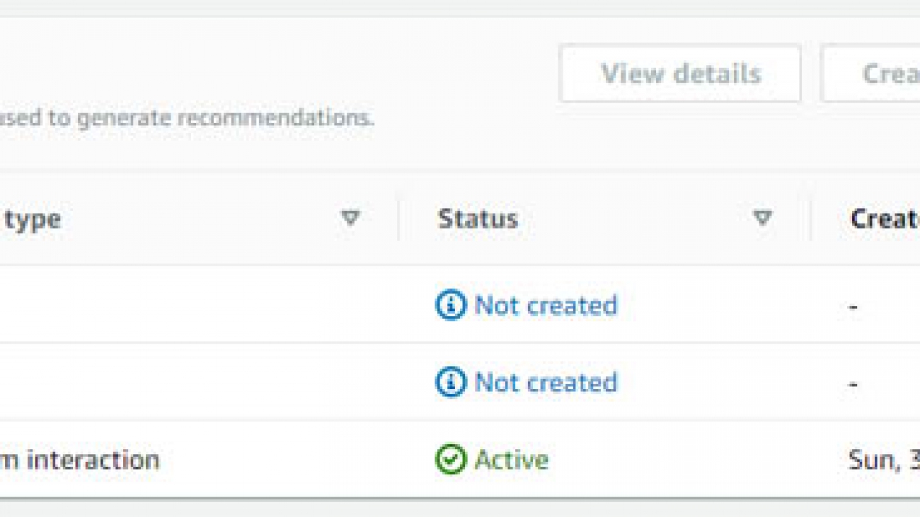
The following screenshot shows the Datasets page on the Amazon Personalize console.

What data types are supported by each category?

Each dataset has a set of required fields, reserved keywords, and required datatypes, as shown in the following table.

Dataset Type Required Fields Reserved Keywords
Users USER_ID (string)
one metadata field
Items ITEM_ID (string)
one metadata field
CREATION_TIMESTAMP (long)


Interactions USER_ID (string)
ITEM_ID (string)
TIMESTAMP (long)

EVENT_TYPE (string)

IMPRESSION (string)

EVENT_VALUE (float, null)


Before you add a dataset to Amazon Personalize, you must define a schema for that dataset. Each dataset type has specific requirements. Schemas in Amazon Personalize are defined in the Avro format.

The following example code shows an interactions schema. The EVENT_TYPE and EVENT_VALUE fields are optional, and are reserved keywords recognized by Amazon Personalize. LOCATION and DEVICE are optional contextual metadata fields.

{
  "type": "record",
  "name": "Interactions",
  "namespace": "com.amazonaws.personalize.schema",
  "fields": [
      {
          "name": "USER_ID",
          "type": "string"
      },
      {
          "name": "ITEM_ID",
          "type": "string"
      },
      {
          "name": "EVENT_TYPE",
          "type": "string"
      },
      {
          "name": "EVENT_VALUE",
          "type": "float"
      },
      {
          "name": "LOCATION",
          "type": "string",
          "categorical": true
      },
      {
          "name": "DEVICE",
          "type": "string",
          "categorical": true
      },
      {
          "name": "TIMESTAMP",
          "type": "long"
      }
  ],
  "version": "1.0"
}

Creating a schema using the AWS Python SDK

To create a schema using the AWS Python SDK, complete the following steps:

  1. Define the Avro format schema that you want to use.
  2. Save the schema in a JSON file in the default Python folder.
  3. Create the schema using the following code:
import boto3

personalize = boto3.client('personalize')

with open('schema.json') as f:
    createSchemaResponse = personalize.create_schema(
        name = 'YourSchema',
        schema = f.read()
    )

schema_arn = createSchemaResponse['schemaArn']

print('Schema ARN:' + schema_arn )

Amazon Personalize returns the ARN of the new schema.

  1. Store the ARN for later use.

Filtering your metadata

Amazon Personalize allows you to experiment with building different models (or solutions) based on different metadata by enabling you to filter records from your interactions dataset and set a threshold for each event type, or simply select and leave out certain event types. You can filter records from an interactions dataset in two ways:

  • Set a threshold to exclude records based on a specific value by specifying an event value in your recipe. If the records include a value that is associated with a specific event—for example, the price a user paid is associated with the purchase of an item—you can set a specific value in a recipe as a threshold to exclude records from training. The amount is called an event value.
  • Exclude records of a certain type by specifying an event type in your recipe. A dataset often includes specific types of activities, for example, purchase, click, or wishlisted. These are called event types. To include only records for specific event types in training, filter your dataset by event type in your recipe.

To filter your metadata, call the CreateSolution API. If you want to specify the event type, for example purchase, set it in the eventType parameter. If you want to specify an event value, for example 10, set it in the eventValueThreshold parameter. You can also specify an event type and an event value. You can specify an eventType, an eventType and eventValueThreshold, or neither. You can’t specify just eventValueThreshold alone. See the following code:

import boto3
 
personalize = boto3.client('personalize')

# Create the solution
create_solution_response = personalize.create_solution(
    name = "your-solution-name",
    datasetGroupArn = dataset_group_arn,
    recipeArn = recipe_arn,
    "eventType": "purchase",
    solutionConfig = {
        "eventValueThreshold": "10"
    }
)

# Store the solution ARN
solution_arn = create_solution_response['solutionArn']

# Use the solution ARN to get the solution status
solution_description = personalize.describe_solution(solutionArn = solution_arn)['solution']
print('Solution status: ' + solution_description['status'])

When selecting metadata for a recommendation engine, it’s helpful to ask the following questions to help guide your decisions:

  • What is likely to be the strongest indicator of a good recommendation—similar users, similar items, or their combined interactions? This can help determine which metadata to select and tag in the datasets. As described, the interactions dataset is the minimum that Amazon Personalize expects, so you have to choose wisely which types of interactions (or events) you want to capture. A combination of interactions and metadata is typically recommended, but choosing which types of interactions to record is important.
  • What is the temporal value of the data? Is old data less potent? How much less? How can you use real-time APIs with real-time data to get the most relevant recommendations that reflect the users’ change of preferences over time?
  • Which metrics best show whether the recommendation engine is working well? Can you align Amazon Personalize metrics with your own KPIs? Can you construct an A/B test with live customers?

The answers to these questions can be a good guide to improve the recommendation system.

Applying metadata selection: Pulselive use case

In a recent engagement with Pulselive, an AWS customer that builds and hosts solutions for large sports organizations, we were asked to aid them in prototyping a personalized recommendation engine for one of their customers, a renowned European football club, to suggest videos to the visitors of their website according to their preferences and past behavior. Their goal was to use all the data they could to provide the website’s visitors with a tailored, highly personalized experience by recommending videos relevant to each user to increase engagement with the content.

Our initial approach was to use some of their existing recorded historical data to extract the minimum required information needed to start building Amazon Personalize solutions that can recommend the right videos to the right users. Therefore, the metadata we initially selected was the simplest form of user-video interactions—clicks—from a historical dataset of which users had clicked on which videos and at what time. We started with 30,000 user interactions.

That allowed us to build a baseline solution that used that information to evaluate the relevance of each video to each user and considered it as our starting point. The next goal was to enrich the dataset by selecting the right metadata and observing the impact that the new models had on user engagement.

At this point, we have to mention that it’s somewhat challenging to predict how well the recommendation system will do when deployed into production. Amazon Personalize provides some standard out-of-the-box metrics when a model has finished training to give you an idea of how well it did at recommending the most relevant items higher on the recommendations list (such as having a high precision or coverage). But you can only evaluate the true impact on your customers when deploying the system into production.

Pulselive chose to do A/B testing, comparing the results of their existing recommendation methods to those produced from an Amazon Personalize campaign. They started with redirecting 5% of their traffic through the Amazon Personalize campaign. After seeing good results, they eventually rolled out to 50% of the traffic being redirected to Amazon Personalize. For more information, see Increasing engagement with personalized online sports content.

Regarding metadata selection, we quickly realized that the users and items in the initial historical dataset weren’t very recent, and most of their IDs didn’t correspond to users and items that had recent activity on their production website.

Luckily, apart from an initial historical dataset, Amazon Personalize can also enrich its models in real time by allowing you to feed in interaction data from your live website. Through the use of the Amazon Personalize PutEvents API, you can record any action users take on the website and feed it into Amazon Personalize in near-real time, updating the model with the most recent user behavior and preferences. This is an important capability because it’s natural for user preferences to change over time, and you don’t want to risk presenting them with items that are either out of date or not relevant to them anymore.

This also means that you can directly connect Amazon Personalize to your website, with no historical data or any models trained, and start feeding in events. After a while, Amazon Personalize has gathered enough data to start making accurate recommendations. For more information, see Recording Events.

We spent some time discussing what other relevant user behavior metadata we could capture, and decided to start recording some to observe whether these would result in a more accurate recommendation system that would impact user engagement on the site. Two simple measures for this were seeing if recommended videos were more frequently visited and watched for longer periods.

We started recording the source of the clicks (recommended list vs. other links in the website), the amount of time a user spent on a clicked video in seconds, and the percentage of the video that time represented (because it’s different for someone to spend 1 minute on a 20-minute video, compared to spending the same time on a 1-minute video to watch it in its entirety). These additions proved to be very important because after a while, user engagement started improving. We discussed and investigated providing more detailed information about user behavior on the website, but decided to pay more attention to the metadata.

Items metadata was important because it allowed Amazon Personalize to have more context on the nature of each video. This ranged from general and broad video categories, such as interviews and games, to more specific categories, such as “Leagues” and “Friendly games,” to more specific metadata, such as which players are featured in a video. Adding metadata about the content for each video significantly improved the personalized recommendations because the solution had a notion of context that helped determine what type on content each user preferred to watch.

Equally, on the user metadata side, more detailed information was provided, trying to capture the demographics and preferences of each user. Of course, in the case of the users, we had to deal with the cold-start problem (new users or guest users for which the system didn’t have any information yet). Luckily, the Amazon Personalize HRNN-Coldstart recipe has proved to be very sufficient in solving this problem by quickly linking the new user’s behavior to existing ones. The more time a guest or new user spends on the platform, the more Amazon Personalize understands about their preferences and adjusts its recommendations accordingly.

We had many options of what type of metadata to include in the interactions dataset, but it’s important to make sure we only use relevant metadata, and we had to pay attention to the balance between providing too much information to a model and providing too little.

For example, we considered recording the movement of each user’s cursors on the website and sending these as well to Amazon Personalize, which in theory could provide a marginal improvement to the performance of the recommendation system. But doing so proved to be expensive and tolling both on the front end (it impacted website performance) and the back end (the volume of data the system had to record, store, and send to Amazon Personalize significantly increased). Therefore, after careful consideration, we decided that cursor movement metadata wasn’t worth keeping.

After a few months, Pulselive rolled out the Amazon Personalize-based recommendation system to nearly half of their customer’s website visitors, and saw that that group’s engagement with their videos increased by 20%.

Conclusion

Recommendation engines can provide more pertinent results to users based on metadata about a user’s historical selections, or on the types of items of interest.

In this post, we looked at how to select the right metadata to get the best results when training a recommendation engine on Amazon Personalize by evaluating which metadata to include and which to exclude. We also looked at a specific use case and how an AWS customer, Pulselive, increased engagement with videos on their customer’s website by providing personalized recommendations to users.

For more information on creating recommendation engines with Amazon Personalize and metadata selection, see the following:


About the Authors

Andrew Hood is a Prototyping Engagement Manager at AWS.


Ion Kleopas is an ML Prototyping Architect at AWS.

Read More

Streamline modeling with Amazon SageMaker Studio and the Amazon Experiments SDK

Streamline modeling with Amazon SageMaker Studio and the Amazon Experiments SDK

The modeling phase is a highly iterative process in machine learning (ML) projects, where data scientists experiment with various data preprocessing and feature engineering strategies, intertwined with different model architectures, which are then trained with disparate sets of hyperparameter values. This highly iterative process with many moving parts can, over time, manifest into a tremendous headache in terms of keeping track of the design decisions applied in each iteration and how the training and evaluation metrics of each iteration compare to the previous versions of the model.

While your head may be spinning by now, fear not! Amazon SageMaker has a solution!

This post walks you through an end-to-end example of using Amazon SageMaker Studio and the Amazon SageMaker Experiments SDK to organize, track, visualize, and compare our iterative experimentation with a Keras model. Although this use case is specific to Keras framework, you can extend the same approach to other deep learning frameworks and ML algorithms.

Amazon SageMaker is a fully managed service, created with the goal of democratizing ML by empowering developers and data scientists to quickly and cost-effectively build, train, deploy, and monitor ML models.

What Is Amazon SageMaker Experiments?

Amazon SageMaker Experiments is a capability of Amazon SageMaker that lets you effortlessly organize, track, compare, and evaluate your ML experiments. Before we dive into the hands-on exercise, let’s first take a step back and review the building blocks of an experiment and their referential relationships. The following diagram illustrates these building blocks.

Figure 1. The building blocks of Amazon SageMaker Experiments

Amazon SageMaker Experiments is composed of the following components:

  • Experiment – An ML problem that we want to solve. Each experiment consists of a collection of trials.
  • Trial An iteration of a data science workflow related to an experiment. Each trial consists of several trial components.
  • Trial component – A stage in a given trial. For instance, as we see in our example, we create one trial component for the data preprocessing stage and one trial component for model training. In a similar fashion, we can also add a trial component for any data postprocessing.
  • Tracker – A mechanism that records various metadata about a particular trial component, including any parameters, inputs, outputs, artifacts, and metrics. A tracker can be linked to a particular training component to assign the collected metadata to it.

Now that we’ve set a rock-solid foundation on the key building blocks of the Amazon SageMaker Experiments SDK, let’s dive into the fun hands-on component.

Prerequisites

You should have an AWS account and a sufficient level of access to create resources in the following AWS services:

Solution overview

As part of this post, we walk through the following high-level steps:

  1. Environment setup
  2. Data preprocessing and feature engineering
  3. Modeling with Amazon SageMaker Experiments
  4. Training and evaluation metric exploration
  5. Environment cleanup

Setting up the environment

We can set up our environment in a few simple steps:

  1. Clone the source code from the GitHub repo, which contains the complete demo, into your Amazon SageMaker Studio environment.
  2. Open the included Jupyter notebook and choose the Python 3 (TensorFlow 2 CPU Optimized)
  3. When the kernel is ready, install sagemaker-experiments package, which enables us to work with the Amazon SageMaker Experiments SDK, and s3fs package, to enable our pandas dataframes to easily integrate with objects in Amazon S3.
  4. Import all required packages and initialize the variables.

The following screenshot shows the environment setup.

Figure 2. Environment Setup

Data preprocessing and feature engineering

Excellent! Now, let’s dive into data preprocessing and feature engineering. In our use case, we use the abalone dataset from the UCI Machine Learning Repository.

Run the steps in the provided Jupyter notebook to complete all data preprocessing and feature engineering. After your data is preprocessed, it’s time for us to seamlessly capture our preprocessing strategy! Let’s create an experiment with the following code:

sm = boto3.client('sagemaker') 
ts = datetime.now().strftime('%Y-%m-%d-%H-%M-%S-%f')

abalone_experiment = Experiment.create(
    experiment_name = 'predict-abalone-age-' + ts,
    description = 'Predicting the age of an abalone based on a set of features describing it',
    sagemaker_boto_client=sm)

Now, we can create a Tracker to describe the Pre-processing Trial Component, including the location of the artifacts:

with Tracker.create(display_name='Pre-processing', sagemaker_boto_client=sm, artifact_bucket=sm_bucket, artifact_prefix=artifacts_path) as tracker:
    tracker.log_parameters({
        'train_test_split': 0.8
    })
    tracker.log_input(name='raw data', media_type='s3/uri', value=source_url)
    tracker.log_output(name='preprocessed data', media_type='s3/uri', value=processed_data_path)
    tracker.log_artifact(name='preprocessors', media_type='s3/uri', file_path='preprocessors.pickle')
    
processing_component = tracker.trial_component

Fantastic! We now have our experiment ready and we’ve already done our due diligence to capture our data preprocessing strategy. Next, let’s dive into the modeling phase.

Modeling with Amazon SageMaker Experiments

Our Keras model has two fully connected hidden layers with a variable number of neurons and variable activation functions. This flexibility enables us to pass these values as arguments to a training job and quickly parallelize our experimentation with several model architectures.

We have mean squared logarithmic error defined as the loss function, and the model is using the Adam optimization algorithm. Finally, the model tracks mean squared logarithmic error as our metric, which automatically propagates into our training trial component in our experiment, as we see shortly:

def model(x_train, y_train, x_test, y_test, args):
    """Generate a simple model"""
    model = Sequential([
                Dense(args.l1_size, activation=args.l1_activation, kernel_initializer='normal'),
                Dense(args.l2_size, activation=args.l2_activation, kernel_initializer='normal'),
                Dense(1, activation='linear')
    ])

    model.compile(optimizer=Adam(learning_rate=args.learning_rate),
                  loss='mean_squared_logarithmic_error',
                  metrics=['mean_squared_logarithmic_error'])
    model.fit(x_train, y_train, batch_size=args.batch_size, epochs=args.epochs, verbose=1)
    model.evaluate(x_test,y_test,verbose=1)

    return model

Fantastic! Follow the steps in the provided notebook to define the hyperparameters for experimentation and instantiate the TensorFlow estimator. Finally, let’s start our training jobs and supply the names of our experiment and trial via the experiment_config dictionary:

abalone_estimator.fit(processed_data_path,
                        job_name=job_name,
                        wait=False,
                        experiment_config={
                                        'ExperimentName': abalone_experiment.experiment_name,
                                        'TrialName': abalone_trial.trial_name,
                                        'TrialComponentDisplayName': 'Training',
                                        })

Exploring the training and evaluation metrics

Upon completion of the training jobs, we can quickly visualize how different variations of the model compare in terms of the metrics collected during model training. For instance, let’s see how the loss has been decreasing by epoch for each variation of the model and observe the model architecture that is most effective in decreasing the loss:

  1. Choose the Amazon SageMaker Experiments List icon on the left sidebar.
  2. Choose your experiment to open it and press Shift to select all four trials.
  3. Choose any of the highlighted trials (right-click) and choose Open in trial component list.
  4. Press Shift to select the four trial components representing the training jobs and choose Add chart.
  5. Choose New chart and customize it to plot the collected metrics that you want to analyze. For our use case, choose the following:
    1. For Data type¸ choose Time series.
    2. For Chart type¸ choose Line.
    3. For X-axis dimension, choose epoch.
    4. For Y-axis, choose loss_TRAIN_last.

Figure 3. Generating plots based on the collected model training metrics

Wow! How quick and effortless was that?! I encourage you to further explore plotting various other metrics on your own. For instance, you can choose the Summary data type to generate a scatter plot and explore if there is a relationship between the size of the first hidden layer in your neural network and the mean squared logarithmic error. See the following screenshot.

Figure 4. Plot of the relationship between the size of the first hidden layer in the neural network and Mean-Squared Logarithmic Error during model evaluation

Next, let’s choose our best-performing trial (abalone-trial-0). As expected, we see two trial components. One represents our data Pre-processing, and the other reflects our model Training. When we open the Training trial component, we see that it contains all the hyperparameters, input data location, Amazon S3 location of this particular version of the model, and more.

Figure 5. Metadata about model training, automatically collected by Amazon SageMaker Experiments

Similarly, when we open the Pre-processing component, we see that it captures where the source data came from, where the processed data was stored in Amazon S3, and where we can easily find our trained encoder and scalers, which we’ve packaged into the preprocessors.pickle artifact.

Figure 6. Metadata about data pre-processing and feature engineering, automatically collected by Amazon SageMaker Experiments

Cleaning up

What a fun exploration this has been! Let’s now clean up after ourselves by running the cleanup function provided at the end of the notebook to hierarchically delete all elements of the experiment that we created in this post:

abalone_experiment.delete_all('--force')

Conclusion

You have now learned to seamlessly track the design decisions that you made during data preprocessing and model training, as well as rapidly compare and analyze the performance of various iterations of your model by using the tracked metrics of the trials in your experiment.

I hope that you enjoyed diving into the intricacies of the Amazon SageMaker Experiments SDK and exploring how Amazon SageMaker Studio smoothly integrates with it, enabling you to lose yourself in experimentation with your ML model without losing track of the hard work you’ve done! I highly encourage you to leverage the Amazon SageMaker Experiments Python SDK in your next ML engagement and I invite you to consider contributing to the further evolution of this open-sourced project.


About the Author

Ivan Kopas is a Machine Learning Engineer for AWS Professional Services, based out of the United States. Ivan is passionate about working closely with AWS customers from a variety of industries and helping them leverage AWS services to spearhead their toughest AI/ML challenges. In his spare time, he enjoys spending time with his family, working out, hanging out with friends and diving deep into the fascinating realms of economics, psychology and philosophy.


Read More

Robust market equilibria: How to model uncertain buyer preferences

Robust market equilibria: How to model uncertain buyer preferences

What we did

The research in our paper “Robust market equilibria with uncertain preferences,” published at AAAI 2020, is motivated by allocation problems in online markets. Real-world examples of online markets include the following:

  • Online advertising: How should ads be allocated to impressions?
  • Ride allocation: How should ride-sharing platforms allocate drivers to riders?
  • Recommendation systems: How should online recommendation systems (for example, Facebook Jobs, which is a jobs recommendation system) allocate job recommendations to viewers?

In all of these examples, the market consists of buyers (i.e., advertisers) and items (i.e., ad impressions). The buyers have preferences, which are captured by their utility functions. When the platform makes an allocation of an item to a buyer, the buyer receives some utility. In exchange, the buyer often makes a payment of a real or fictitious currency. The allocation rule (who gets what) and the payment rules (pricing of the items) involved are important design choices because they influence whether participants in the market find satisfaction by participating.

A rich body of work, originally by Eisenberg and Gale (1959) in economics and computer science, investigates questions like these. The main insight is the introduction of the notion of a market equilibrium — wherein allocations and prices are determined so that each buyer is “satisfied” with the outcome.

An important challenge within this context is that markets are highly uncertain. At large scales (think billions of buyers and items), it is practically impossible to know the preferences of each buyer perfectly. (This theme has been extensively investigated in “Computing large market equilibria using abstractions,“ and is in a sense a starting point for this work.) In practice, platforms will have machine learning models to predict these preferences from extremely sparse data. These machine learning models are imperfect and make errors in prediction. The challenge we seek to investigate is how do we make allocation and pricing decisions in the face of this uncertainty?

Ideally, we would like our allocation and pricing decisions to be robust against the uncertainty. That is to say, we would like it so that buyers remain “satisfied” when the platform makes decisions with uncertain data. To that end, the work described in our recent paper extends the notion of a market equilibrium to the notion of a robust market equilibrium (RME). The focus of the paper is developing computational tools for RME, as well as applications of the same on some real-world data sets.

How we did it

We start with the decades-old result by Eisenberg and Gale, which answers the question of how to compute market equilibria. (As a caveat, we exclusively work in the so-called divisible goods setting.) They propose doing so by solving a convex optimization program that involves maximizing the geometric mean of all agents’ utilities (also known as Nash Welfare) subject to resource constraints. The key intuition here is that maximizing the geometric mean ensures that allocations cannot be too biased against any individual agent. For example, if we allocate no items to any individual agent, the Nash Welfare is zero.

An analysis of the optimality conditions of the Eisenberg-Gale convex program immediately reveals a host of attractive properties, including the proof that the resulting solution is a market equilibrium.

In order to model uncertain markets, we view the parameters (i.e., the utilities) of agents participating in the market as uncertain. There are many different ways of modeling this uncertainty, resulting in different uncertainty models. We propose and investigate a few natural models in our paper.

We then bring in the main idea of the paper, i.e., the application of a technique called robust optimization to the Eisenberg-Gale convex program. Robust optimization, which is a fairly mature subarea within optimization, deals with solving uncertain optimization problems. In a typical robust optimization problem, the parameters of the problem (the cost function and constraints) are uncertain — or they could be adversarially chosen from a known set.

The technique of robust optimization then seeks to find a solution that produces the best outcome possible against the (worse-case) adversarial choice of parameters from the uncertainty set. Interestingly, many classes of robust optimization problems (including the EG program, as we show in our paper) can be reformulated as (vanilla, certain) optimization problems via convex duality.

After applying the technique of robust optimization, we show a few interesting economic properties of the “robustified” Eisenberg-Gale convex program. One such result is that the solution of the robust variant can be thought of as another market equilibrium where each individual buyer seeks to maximize their uncertain utilities robustly — or, in other words, gain as much utility as possible in the face of adversarial uncertainty. Robust counterparts of a number of other classical properties also follow.

Next, we’ll discuss the application of these ideas to a real-world data set that provides preference information in a recommendation system, namely the MovieLens data set. We perform a thought experiment where we have users choosing movies, with the MovieLens data set indicating how much utility a user would get by watching a particular movie. However, there is a limited supply of movies, so then we would like to allocate movies judiciously, which is using a market equilibrium.

Figure 1
Figure 1 shows the behavior of the Nash Welfare (y-axis) as the size of the uncertainty set (x-axis) grows. The blue line shows the Nash Welfare if we had ignored the uncertainty and simply used the equilibrium based on the Eisenberg-Gale program. The green line shows the Nash Welfare when using the robust solution. There are two trends to note: First, the performance degrades as uncertainty increases, as expected. Second, by a widening margin, the robust solution outperforms the uncertainty-agnostic solution.

Other aspects of the solution can also be investigated. As an example, we consider robust envy — which is a measure of how dissatisfied users are with their own allocation of movies, relative to others under preference uncertainty — can be compared in the uncertain market when using the robust against the vanilla solution.

Figure 2
In Figure 2, the green plot shows the distribution of users’ robust envy using the robust solution in comparison with the blue plot, which shows distribution of envy when using the uncertainty-agnostic solution. The robust envy is significantly lower.

In conclusion, the numerical results reaffirm that modeling uncertainty and accounting for the same when designing allocations result in better market allocations overall.

What’s next

One of our main follow-up questions is how to make such allocations in an online setting. Many practical applications of interest (such as recommender systems) make decisions online, where instead of seeing an entire view of the market and then making allocations, users and buyers arrive online and allocations must be made instantly. Further practical challenges include making allocation decisions within fractions of a second (very low latency), where solving convex optimization problems becomes infeasible.

In conclusion, our research shows that modeling and accounting for uncertainty in markets can dramatically impact the quality of allocations. We introduce the notion of an RME that is uncertainty-aware, show how to compute it numerically, and demonstrate that this uncertainty-aware allocation method is superior to more agnostic allocation methods.

The post Robust market equilibria: How to model uncertain buyer preferences appeared first on Facebook Research.

Read More

Provably exact artificial intelligence for nuclear and particle physics

The Standard Model of particle physics describes all the known elementary particles and three of the four fundamental forces governing the universe; everything except gravity. These three forces — electromagnetic, strong, and weak — govern how particles are formed, how they interact, and how the particles decay.

Studying particle and nuclear physics within this framework, however, is difficult, and relies on large-scale numerical studies. For example, many aspects of the strong force require numerically simulating the dynamics at the scale of 1/10th to 1/100th the size of a proton to answer fundamental questions about the properties of protons, neutrons, and nuclei.

“Ultimately, we are computationally limited in the study of proton and nuclear structure using lattice field theory,” says assistant professor of physics Phiala Shanahan. “There are a lot of interesting problems that we know how to address in principle, but we just don’t have enough compute, even though we run on the largest supercomputers in the world.”

To push past these limitations, Shanahan leads a group that combines theoretical physics with machine learning models. In their paper “Equivariant flow-based sampling for lattice gauge theory,” published this month in Physical Review Letters, they show how incorporating the symmetries of physics theories into machine learning and artificial intelligence architectures can provide much faster algorithms for theoretical physics. 

“We are using machine learning not to analyze large amounts of data, but to accelerate first-principles theory in a way which doesn’t compromise the rigor of the approach,” Shanahan says. “This particular work demonstrated that we can build machine learning architectures with some of the symmetries of the Standard Model of particle and nuclear physics built in, and accelerate the sampling problem we are targeting by orders of magnitude.” 

Shanahan launched the project with MIT graduate student Gurtej Kanwar and with Michael Albergo, who is now at NYU. The project expanded to include Center for Theoretical Physics postdocs Daniel Hackett and Denis Boyda, NYU Professor Kyle Cranmer, and physics-savvy machine-learning scientists at Google Deep Mind, Sébastien Racanière and Danilo Jimenez Rezende.

This month’s paper is one in a series aimed at enabling studies in theoretical physics that are currently computationally intractable. “Our aim is to develop new algorithms for a key component of numerical calculations in theoretical physics,” says Kanwar. “These calculations inform us about the inner workings of the Standard Model of particle physics, our most fundamental theory of matter. Such calculations are of vital importance to compare against results from particle physics experiments, such as the Large Hadron Collider at CERN, both to constrain the model more precisely and to discover where the model breaks down and must be extended to something even more fundamental.”

The only known systematically controllable method of studying the Standard Model of particle physics in the nonperturbative regime is based on a sampling of snapshots of quantum fluctuations in the vacuum. By measuring properties of these fluctuations, once can infer properties of the particles and collisions of interest.

This technique comes with challenges, Kanwar explains. “This sampling is expensive, and we are looking to use physics-inspired machine learning techniques to draw samples far more efficiently,” he says. “Machine learning has already made great strides on generating images, including, for example, recent work by NVIDIA to generate images of faces ‘dreamed up’ by neural networks. Thinking of these snapshots of the vacuum as images, we think it’s quite natural to turn to similar methods for our problem.”

Adds Shanahan, “In our approach to sampling these quantum snapshots, we optimize a model that takes us from a space that is easy to sample to the target space: given a trained model, sampling is then efficient since you just need to take independent samples in the easy-to-sample space, and transform them via the learned model.”

In particular, the group has introduced a framework for building machine-learning models that exactly respect a class of symmetries, called “gauge symmetries,” crucial for studying high-energy physics.

As a proof of principle, Shanahan and colleagues used their framework to train machine-learning models to simulate a theory in two dimensions, resulting in orders-of-magnitude efficiency gains over state-of-the-art techniques and more precise predictions from the theory. This paves the way for significantly accelerated research into the fundamental forces of nature using physics-informed machine learning.

The group’s first few papers as a collaboration discussed applying the machine-learning technique to a simple lattice field theory, and developed this class of approaches on compact, connected manifolds which describe the more complicated field theories of the Standard Model. Now they are working to scale the techniques to state-of-the-art calculations.

“I think we have shown over the past year that there is a lot of promise in combining physics knowledge with machine learning techniques,” says Kanwar. “We are actively thinking about how to tackle the remaining barriers in the way of performing full-scale simulations using our approach. I hope to see the first application of these methods to calculations at scale in the next couple of years. If we are able to overcome the last few obstacles, this promises to extend what we can do with limited resources, and I dream of performing calculations soon that give us novel insights into what lies beyond our best understanding of physics today.”

This idea of physics-informed machine learning is also known by the team as “ab-initio AI,” a key theme of the recently launched MIT-based National Science Foundation Institute for Artificial Intelligence and Fundamental Interactions (IAIFI), where Shanahan is research coordinator for physics theory.

Led by the Laboratory for Nuclear Science, the IAIFI is comprised of both physics and AI researchers at MIT and Harvard, Northeastern, and Tufts universities.

“Our collaboration is a great example of the spirit of IAIFI, with a team with diverse backgrounds coming together to advance AI and physics simultaneously” says Shanahan. As well as research like Shanahan’s targeting physics theory, IAIFI researchers are also working to use AI to enhance the scientific potential of various facilities, including the Large Hadron Collider and the Laser Interferometer Gravity Wave Observatory, and to advance AI itself. 

Read More

Expanding Amazon Lex conversational experiences with US Spanish and British English

Expanding Amazon Lex conversational experiences with US Spanish and British English

Amazon Lex provides the power of automatic speech recognition (ASR) for converting speech to text, along with natural language understanding (NLU) for recognizing user intents. This combination allows you to develop sophisticated conversational interfaces using both voice and text for chatbots, IVR bots, and voicebots.

This week, we’re announcing Amazon Lex support for British English and US Spanish. With British English, your conversational bots can be localized to understand the British English accent, while delivering responses in Amazon Polly voices designed to sound like UK English speakers. Brilliant!

With support for US Spanish, you can develop applications for the second-most widely spoken language in the United States. Amazon Lex can now accurately recognize written and spoken Spanish, while providing responses using Amazon Polly’s natural sounding US Spanish voices. Listo!

In this post, we consider a hypothetical appliance manufacturer in the United States. Customers calling into their service center to schedule or change a repair appointment may prefer to speak in English or Spanish. The application for this use case allows callers to select their preferred language by saying “English” or “Español” when prompted. You want to provide them with the best customer service experience, no matter whether it is their washing machine or their lavadora that needs repair.

We show you how to create an Amazon Connect call center experience that supports both US English and US Spanish. Customers can schedule, change, and cancel appointments, using a fully automated solution that converses with them in their preferred language.

Building a multi-language conversational experience

This post uses the following sample conversations:

Agent: Thank you for calling. To continue in English, say “English,” for Spanish, say “Español.”

US English

Agent: I can schedule or change a repair appointment. How can I help?

User: I want to get my dishwasher fixed.

Agent: What city are you in?

User: Philadelphia

Agent: I have technicians available next week. When would you prefer to have them visit?

User: September 24th at noon

Agent: OK, you are all set for your dishwasher repair in Philadelphia on the 24th of September at noon.

US Spanish

Agent: Puede reservar o cambiar una cita de reparación. ¿Cómo puedo ayudar?

User: Me gustaria programar una cita

Agent: Para qué tipo de aparato?

User: Refrigerador

Agent: En que ciudad estas?

User: Brooklyn

Agent: En que fecha te gustaria que vinieran?

User: 24 de Septiembre

Agent: Bien, ya está todo listo para la reparación de su refrigerador en 24 de Septiembre, 2020.

To support these conversation models, you need to create Lex bots with relevant user intents. In this post, we create intents for ScheduleAppointment, ModifyAppointment, and CancelAppointment (and in Spanish, ReservarCita, ModificarCita, CancelarCita).

Deploying the sample Lex bots

To create the sample bots, perform the following steps. For this post, you create two Amazon Lex bots: AppointmentBot_enUS for US English, and AppointmentBot_esUS for US Spanish. To follow along with this post, you can create these Lex bots yourself on the Amazon Lex console, or import them directly.

  1. To import the bots, download the US English bot and the US Spanish bot
  2. On the Amazon Lex console, choose
  3. Select the zip that you downloaded, and choose Import.
  4. When the import process is complete, choose AppointmentBot_enUS, and choose
  5. When the build it complete, go back to the Amazon Lex console main window, and choose Import.
  6. Select the zip that you downloaded, and choose Import.
  7. When the import process is complete, choose AppointmentBot_esUS, and choose

At this point, you should have two working Lex bots: one for US English, and one for US Spanish.

Creating your Amazon Connect instance

In this section, we integrate the bots with an Amazon Connect cloud-based call center instance. The first step is to create the Amazon Connect instance:

  1. On the AWS Management Console, choose Amazon Connect.
  2. If this is your first Amazon Connect instance, choose Get started; otherwise, choose Add an instance.
  3. For Identity management, choose Store users within Amazon Connect.
  4. Enter a URL prefix, such as appointment-bot-############, where ############ is your current AWS account number.
  5. Choose Next step.
  6. For Create an administrator, enter a name, password, and email address.
  7. Choose Next step.
  8. For Telephony Options, leave both call options selected by default.
  9. Choose Next step.
  10. For Data storage, choose Next step.
  11. Review the settings and choose Create instance.

Associating your bots with your Amazon Connect instance

Now that you have an Amazon Connect instance, you can claim a phone number, create a contact flow, and integrate your contact flow with the two Lex bots you created in the prior step. First, associate your bots with your Amazon Connect instance:

  1. On the Amazon Connect console, open your instance by choosing the Instance Alias
  2. Choose Contact flows.
  3. From the drop-down list, choose AppointmentBot_enUS. If you don’t see the bot in the list, make sure you have selected the same Region you used when you created your Lex bot.
  4. Choose + Add Lex Bot.
  5. From the drop-down list, choose AppointmentBot_esUS and choose + Add Lex Bot.

Configuring Amazon Connect to work with your bot

Now you can use your bots with Amazon Connect. First, claim a phone number for your Amazon Connect instance:

  1. On the Amazon Connect console, choose Overview.
  2. Choose the Amazon Connect
  3. Choose the Login URL link, and enter the user name and password you specified earlier.
  4. On the Amazon Connect console, for Step 1, Choose Begin.
  5. For your phone number, choose a country, Direct Dial or Toll Free, and a phone number.
  6. Choose Next.
  7. If you want to test your new phone number, try it on the next screen or choose Skip for now.

For this post, you can skip the hours of operation, creating queues, and creating prompts. For more information on these features, see the Amazon Connect Administrator Guide. Now let’s import the contact flow.

  1. Download and unzip the sample Amazon Connect contact flow for this post: manage_repairs.zip.
  2. On the Amazon Connect console, go to Step 5, Create contact flows, choose View contact flows.
  3. Choose Create contact flow.
  4. From the drop-down at the top right side of the page, choose Import flow (beta).
  5. Choose Select and select the manage-repairs.json file you downloaded, and select Import.
  6. Choose Save, and then Publish.

Your contact flow should look like the following screenshot.

  1. Choose the Routing icon from the side menu, and choose Phone numbers.
  2. Choose your phone number to edit it, and change the contact flow or IVR to the Manage Repairs contact flow you just created.
  3. Choose Save.

Your Amazon Connect instance is now configured to work with your Amazon Lex bots. Try calling the phone number to see how it works!

Conclusion

With the addition of British English and US Spanish language support, along with US English and Australian English, Amazon Lex allows you to create bots that can converse with users in their native language. You can combine Amazon Lex with Amazon Connect to create streamlined, multi-language call center user experiences in minutes. The additional language support in Amazon Lex is available at the same price, and in the same Regions, as US English. You can try these languages via the console, the AWS Command Line Interface (AWS CLI), and the AWS SDKs.


About the Authors

Claire Mitchell is a Design Consultant with the AWS Professional Services Conversational AI team. Occasionally she spends time exploring speculative design practices, textiles, and playing the drums.


Brian Yost is a Senior Consultant with the AWS Professional Services Conversational AI team. In his spare time, he enjoys mountain biking, home brewing, and tinkering with technology.


As a Product Manager on the Amazon Lex team, Harshal Pimpalkhute spends his time trying to get machines to engage (nicely) with humans.


Read More

Modeled Behavior: dSPACE Introduces High-Fidelity Vehicle Dynamics Simulation on NVIDIA DRIVE Sim

Modeled Behavior: dSPACE Introduces High-Fidelity Vehicle Dynamics Simulation on NVIDIA DRIVE Sim

When it comes to autonomous vehicle simulation testing, every detail must be on point.

With its high-fidelity automotive simulation model (ASM) on NVIDIA DRIVE Sim, global automotive supplier dSPACE is helping developers keep virtual self-driving true to the real world. By combining the modularity and openness of the DRIVE Sim simulation software platform with highly accurate vehicle models like dSPACE’s, every minor aspect of an AV can be thoroughly recreated, tested and validated.

The dSPACE ASM vehicle dynamics model makes it possible to simulate elements of the car — suspension, tires, brakes — all the way to the full vehicle powertrain and its interaction with the electronic control units that power actions such as steering, braking and acceleration.

As the world continues to work from home, simulation has become an even more crucial tool in autonomous vehicle development. However, to be effective, it must be able to translate to real-world driving.

dSPACE’s modeling capabilities are key to understanding vehicle behavior in diverse conditions, enabling the exhaustive and high-fidelity testing required for safe self-driving deployment.

Detailed Validation

High-fidelity simulation is more than just a realistic-looking car driving in a recreated traffic scenario. It means in any given situation, the simulated vehicle will behave just as a real vehicle driving in the real world would.

If an autonomous vehicle suddenly brakes on a wet road, there are a range of forces that affect how and where the vehicle stops. It could slide further than intended or fishtail, depending on the weather and road conditions. These possibilities require the ability to simulate dynamics such as friction and yaw, or the way the vehicle moves vertically.

The dSPACE ASM vehicle dynamics model includes these factors, which can then be compared with a real vehicle in the same scenario. It also tests how the same model acts in different simulation environments, ensuring consistency with both on-road driving and virtual fleet testing.

A Comprehensive and Diverse Platform

The NVIDIA DRIVE Sim platform taps into the computing horsepower of NVIDIA RTX GPUs to deliver a revolutionary, scalable, cloud-based computing platform, capable of generating billions of qualified miles for autonomous vehicle testing.

It’s open, meaning both users and partners can incorporate their own models in simulation for comprehensive and diverse driving scenarios.

dSPACE chose to integrate its vehicle dynamics ASM with DRIVE Sim due to its ability to scale for a wide range of testing conditions. When running on the NVIDIA DRIVE Constellation platform, it can perform both software-in-the-loop and hardware-in-the-loop testing, which includes the in-vehicle AV computer controlling the vehicle in the simulation process. dSPACE’s broad expertise and long track-record in hardware-in-the-loop simulation make for a seamless implementation of ASM on DRIVE Constellation.

Learn more about the dSPACE ASM vehicle dynamics in the DRIVE Sim platform at the company’s upcoming GTC sessionregister before Sept. 25 to receive Early Bird pricing.

The post Modeled Behavior: dSPACE Introduces High-Fidelity Vehicle Dynamics Simulation on NVIDIA DRIVE Sim appeared first on The Official NVIDIA Blog.

Read More