For many organizations, consolidating information assets and making them available to employees when needed remains a challenge. Commonly used technology like spreadsheets, relational databases, and NoSQL databases exacerbate this issue by creating more and more unconnected, unstructured data.
Knowledge graphs can provide easier access and understanding to this data by organizing this data and capturing dataset semantics, properties, and relationships. While some organizations use knowledge graphs like Amazon Neptune to add structure to their data, they still lack a targeted search engine that users can leverage to search this information.
Amazon Kendra is an intelligent search service powered by machine learning. Kendra reimagines enterprise search for your websites and applications so your employees and customers can easily find the content they are looking for, even when it’s scattered across multiple locations and content repositories within your organization.
This solution illustrates how to create an intelligent search engine on AWS using Amazon Kendra to search a knowledge graph stored in Amazon Neptune. We illustrate how you can provision a new Amazon Kendra index in just a few clicks – no prior Machine Learning (ML) experience required! We then show how an existing knowledge graph stored in Amazon Neptune can be connected to Amazon Kendra’s pipeline as metadata as well as into the knowledge panels to build a targeted search engine. Knowledge panels are information boxes that appear on search engines when you search for entities (people, places, organizations, things) that are contained in the knowledge graph. Finally, this solution provides you with a ranked list of the top notable entities that match certain criteria and finds more relevant search results extracted from the knowledge graph.
The following are several common use cases for integrating an enterprise search engine with a knowledge graph:
- Add a knowledge graph as metadata to Amazon Kendra to more relevant results
- Derive a ranked list of the top notable entities that match certain criteria
- Predictively complete entities in a search box
- Annotate or organize content using the knowledge graph entities by querying in Neptune
Required Services
In order to complete this solution, you will require the following:
Sample dataset
For this solution, we use a subset of the Arbitration Awards Online database, which is publicly available. Arbitration is an alternative to litigation or mediation when resolving a dispute. Arbitration panels are composed of one or three arbitrators who are selected by the parties. They read the pleadings filed by the parties, listen to the arguments, study the documentary and testimonial evidence, and render a decision.
The panel’s decision, called an award, is final and binding on all the parties. All parties must abide by the award, unless it’s successfully challenged in court within the statutory time period. Arbitration is generally confidential, and documents submitted in arbitration are not publicly available, unlike court-related filings.
However, if an award is issued at the conclusion of the case, the Financial Industry Regulatory Authority (FINRA) posts it in its Arbitration Awards Online database, which is publicly available. We use a subset of this dataset for our use case under FINRA licensing (©2020 FINRA. All rights reserved. FINRA is a registered trademark of the Financial Industry Regulatory Authority, Inc. Reprinted with permission from FINRA) to create a knowledge graph for awards.
Configuring your document repository
Before you can create an index in Amazon Kendra, you need to load documents into an S3 bucket. This section contains instructions to create an S3 bucket, get the files, and load them into the bucket. After completing all the steps in this section, you have a data source that Amazon Kendra can use.
- On the AWS Management Console, in the Region list, choose US East (N. Virginia) or any Region of your choice that Amazon Kendra is available in.
- Choose Services.
- Under Storage, choose S3.
- On the Amazon S3 console, choose Create bucket.
- Under General configuration, provide the following information:
- Bucket name –
enterprise-search-poc-ds-UNIQUE-SUFFIX
- Region – Choose the same Region that you use to deploy your Amazon Kendra index (this post uses US East (N. Virginia)
us-east-1)
- Under Bucket settings for Block Public Access, leave everything with the default values.
- Under Advanced settings, leave everything with the default values.
- Choose Create bucket.
- Download kendra-graph-blog-data and unzip the files.
- Upload the
index_data folder from the unzipped files.
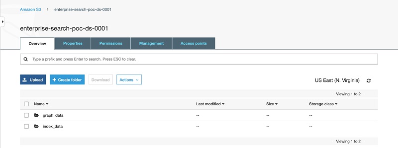
Inside your bucket, you should now see two folders: index_data (with 20 objects) and graph_data (with two objects).
The following screenshot shows the contents of enterprise-search-poc-ds-UNIQUE-SUFFIX.
The following screenshot shows the contents of index_data.
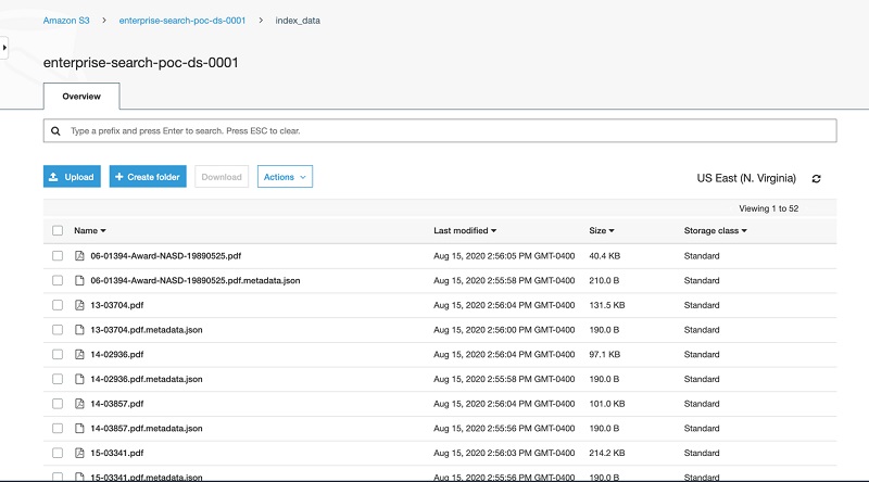
The index_data folder contains two files: an arbitration PDF file and arbitration metadata file.
The following code is an example for arbitration metadata. DocumentId is the arbitration case number, and we use this identifier to create a correlation between the Amazon Kendra index and a graph dataset that we load into Neptune.
{
  "DocumentId": "17-00486",
  "ContentType": "PDF",
  "Title": "17-00486",
  "Attributes": {
    "_source_uri": "https://www.finra.org/sites/default/files/aao_documents/17-00486.pdf"
  }
}
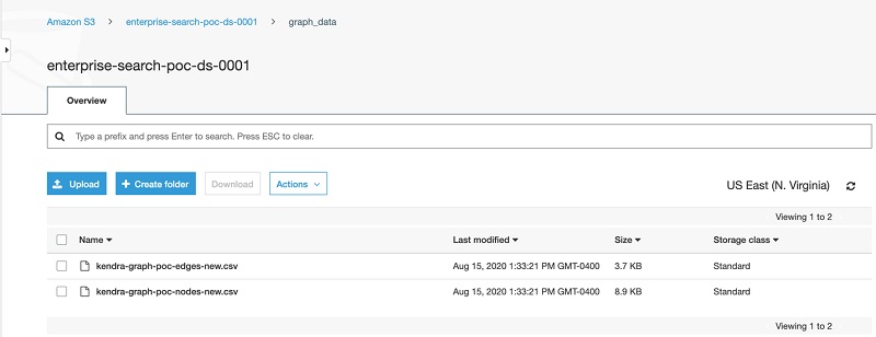
The following screenshot shows the contents of graph_data.
Setting up an Amazon Kendra index
In this section, we set up an Amazon Kendra index and configure an S3 bucket as the data source.
- Sign in to the console and confirm that you have set the Region to
us-east-1.
- Navigate to the Amazon Kendra service and choose Launch Amazon Kendra.
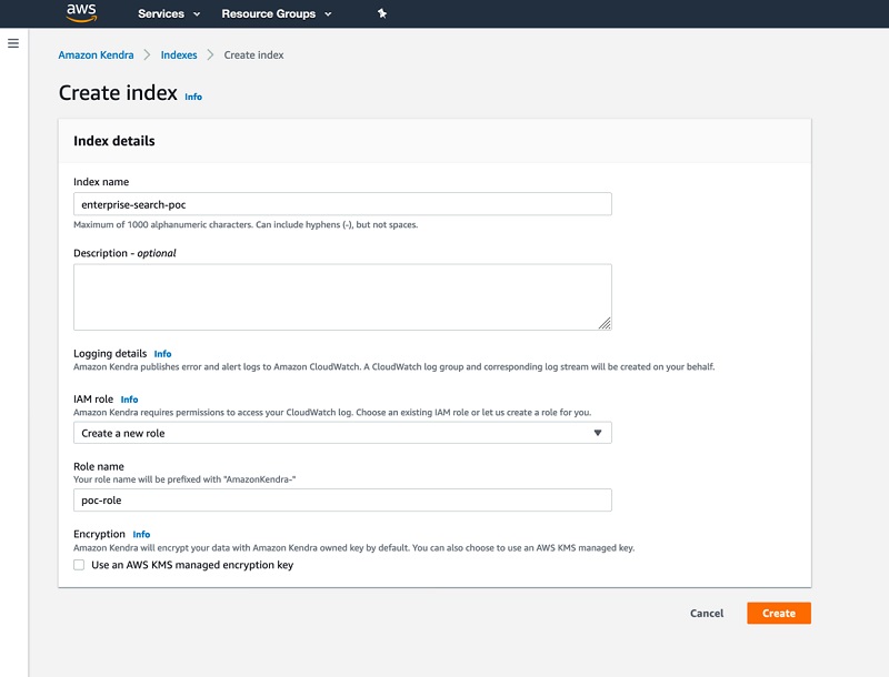
- For Index name, enter
enterprise-search-poc.
- For IAM role, choose Create a new role.
- For Role name, enter
poc-role.
- Leave Use an AWS KMS managed encryption key
- Choose Create.
The index creation may take some time. For more information about AWS Identity and Access Management (IAM) access roles, see IAM access roles for Amazon Kendra.
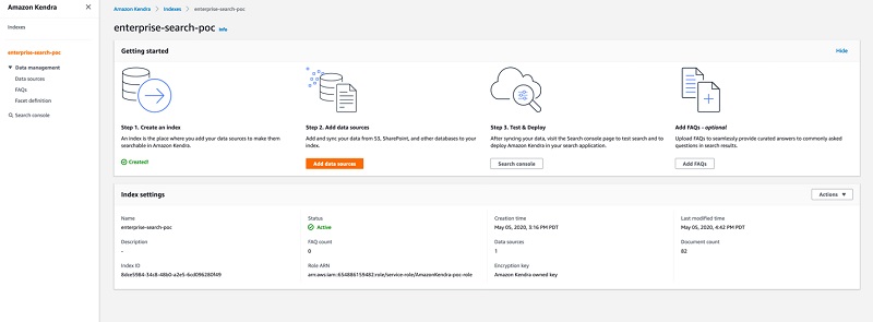
- When index creation is complete, on the Amazon Kendra console, choose your new index.
- In the Index settings section, locate the index ID.
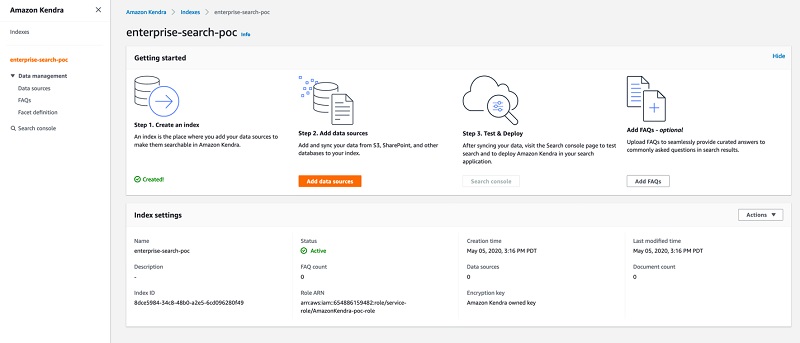
You use the index ID in a later step.
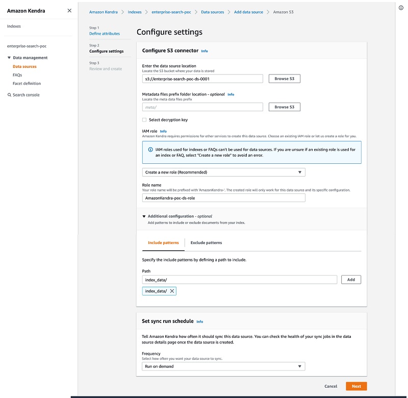
Adding a data source
To add your data source, complete the following steps:
- On the Amazon Kendra console, choose your index.
- Choose Add data source.
- For Select connector type for your data source, choose Add connector under Amazon S3.
- For Data source name, enter a name for your data source (for example,
ent-search-poc-ds-001).
- For Enter the data source location, choose Browse S3 and choose the bucket you created earlier.
- For IAM role, choose Create new role.
- For Role name, enter
poc-ds-role.
- In the Additional configuration section, on the Include pattern tab, add
index_data.
- In the Set sync run schedule section, choose Run on demand.
- Choose Next.
- Review your details and choose Create.
- In the details page of your data source, choose Sync now.
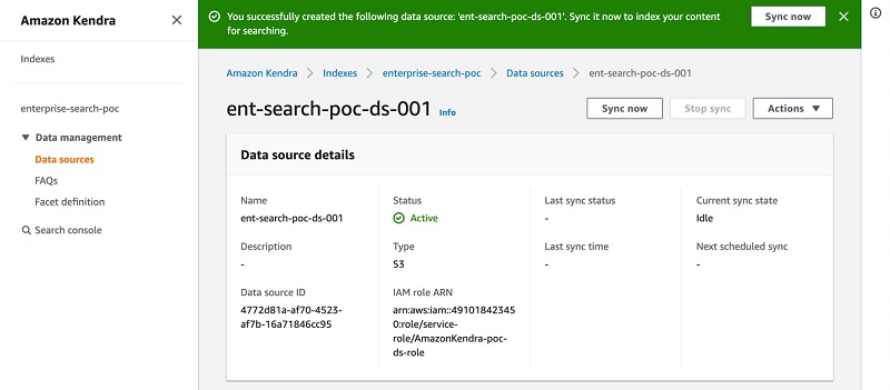
Kendra starts crawling and indexing the data source from Amazon S3 and prepares the index.
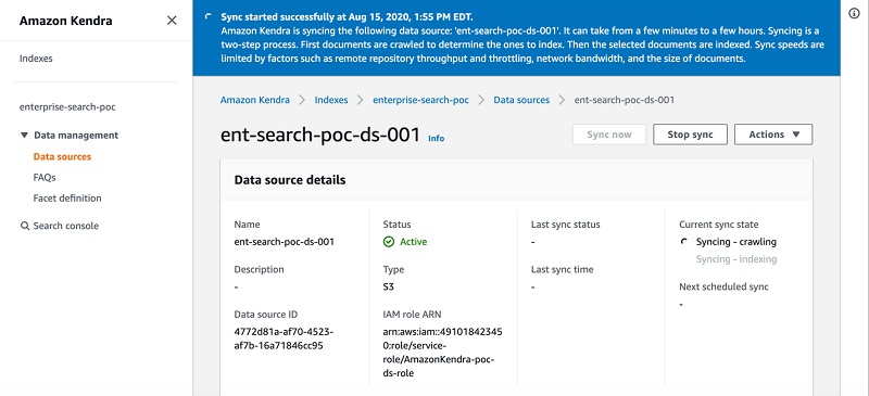
You can also monitor the process on Amazon CloudWatch.
Searching the ingested documents
To test the index, complete the following steps:
- On the Amazon Kendra console, navigate to your index.
- Choose Search console.
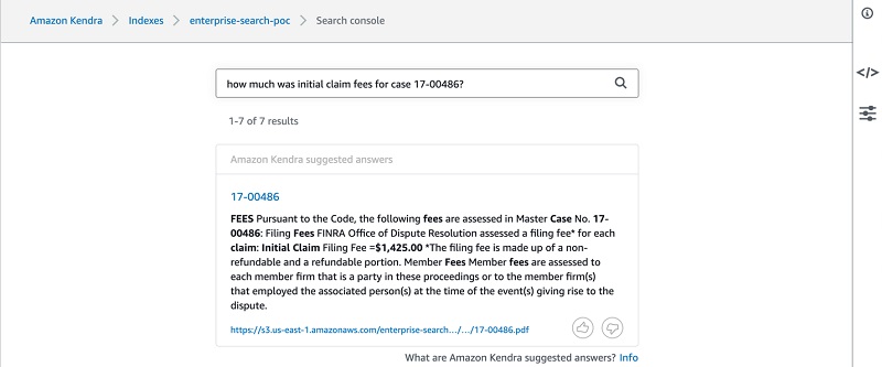
- Enter a question (for example, how much was initial claim fees for case 17-00486?).
The following screenshot shows your search results.
Knowledge graph
This section describes a knowledge graph of the entities and relationships that participate in arbitration panels. We use Apache TinkerPop Gremlin format to load the data to Neptune. For more information, see Gremlin Load Data Format.
To load Apache TinkerPop Gremlin data using the CSV format, you must specify the vertices and the edges in separate files. The loader can load from multiple vertex files and multiple edge files in a single load job.
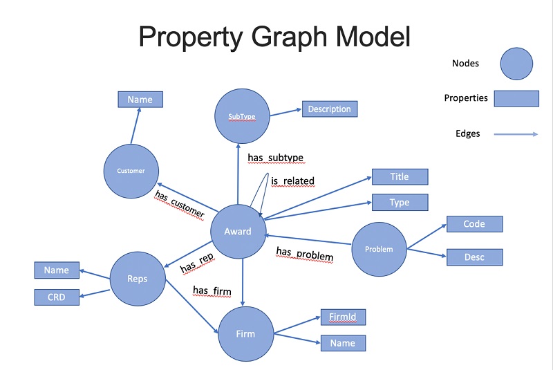
The following diagram shows the graph ontology. Each award has properties, such as Problem, Customer, Representative, Firm, and Subtype. The is_related edge shows relationships between awards.
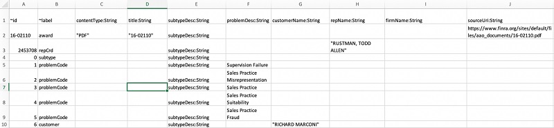
You can access the CSV files for both vertex and nodes in the enterprise-search-poc.zip file. The following screenshot shows a tabular view of the vertex file.
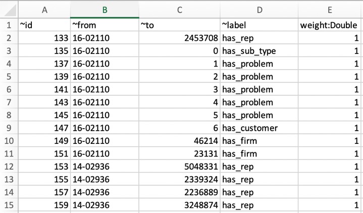
The following screenshot shows a tabular view of the edge file.
Launching the Neptune-SageMaker stack
You can launch the Neptune-SageMaker stack from the AWS CloudFormation console by choosing Launch Stack:
| Region |
View |
Launch |
US East 1
(N. Virginia) |
View |
 |
Acknowledge that AWS CloudFormation will create IAM resources, and choose Create.
The Neptune and Amazon SageMaker resources described here incur costs. With Amazon SageMaker hosted notebooks, you pay simply for the Amazon Elastic Compute Cloud (Amazon EC2) instance that hosts the notebook. For this post, we use an ml.t2.medium instance, which is eligible for the AWS free tier.
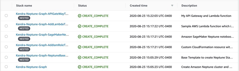
The solution creates five stacks, as shown in the following screenshot.
Browsing and running the content
After the stacks are created, you can browse your notebook instance and run the content.
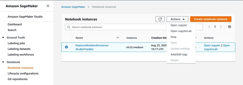
- On the Amazon SageMaker console, choose Notebook instances on the navigation pane.
- Select your instance and from the Actions menu, choose Open Jupyter.
- In the Jupyter window, in the Neptune directory, open the
Getting-Starteddirectory.
The Getting-Starteddirectory contains three notebooks:
01-Introduction.ipynb02-Labelled-Property-Graph.ipynb03-Graph-Recommendations.ipynb
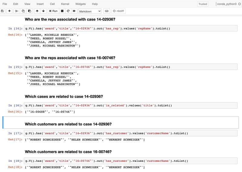
The first two introduce Neptune and the property graph data model. The third contains an runnable example of an arbitration knowledge graph recommendation engine. When you run the content, the notebook populates Neptune with a sample award dataset and issues several queries to generate related cases recommendations.
- To see this in action, open
03-Graph-Recommendations.ipynb.
- Change the
bulkLoad Amazon S3 location to your created Amazon S3 location (enterprise-search-poc-ds-UNIQUE-SUFFIX).
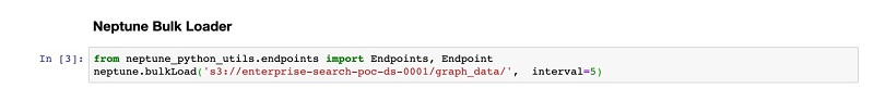
- Run each cell in turn, or choose Run All from the Cell drop-down menu.
You should see the results of each query printed below each query cell (as in the following screenshot).
Architecture overview
DocumentId in Amazon Kendra is the key for an Amazon Kendra index and knowledge graph data. DocumentId in an Amazon Kendra index should be the same as ~id in the graph node. This creates the association between the Amazon Kendra results and graph nodes. The following diagram shows the architecture for integrating Amazon Kendra and Neptune.
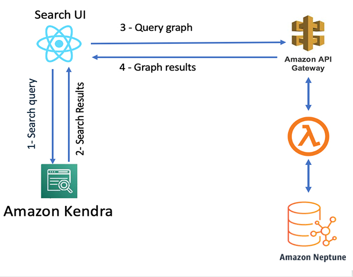
The architecture workflow includes the following steps:
- The search user interface (UI) sends the query to Amazon Kendra.
- Amazon Kendra returns results based on its best match.
- The UI component calls Neptune via Amazon API Gateway and AWS Lambda with the
docId as the request parameter.
- Neptune runs the query and returns all related cases with the requested
docId.
- The UI component renders the knowledge panel with the graph responses.
Testing Neptune via API Gateway
To test Neptune via API Gateway, complete the following steps:
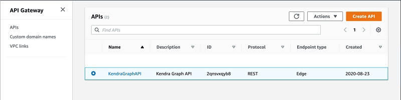
- On the API Gateway console, choose APIs.
- Choose KendraGraphAPI to open the API page.
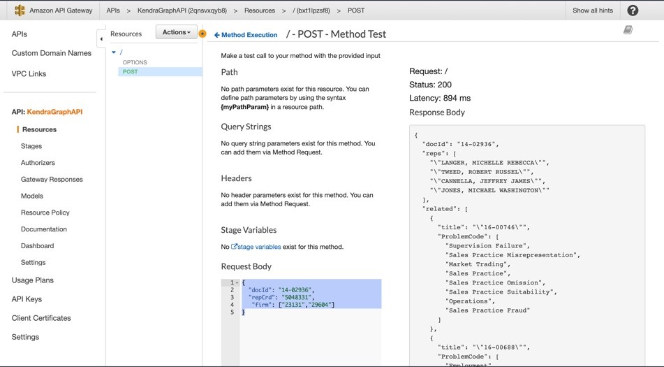
- Select the POST method and choose Test.
- Enter the following sample event data:
{
  "docId": "14-02936",
  "repCrd": "5048331",
  "firm": ["23131","29604"]
}
- Choose Test.
This sends an HTTP POST request to the endpoint, using the sample event data in the request body. In the following screenshot, the response shows the related cases for award 14-02936.
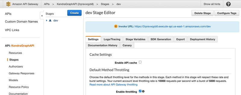
- On the navigation name, choose Stages.
- Choose dev.
- Copy the Invoke URL value and save it to use in the next step.
- To test the HTTP, enter the following CURL command. Replace the endpoint with your API Gateway invoke URL.
curl --location --request POST 'REPLACE_WITH_API_GATEWAY_ENDPOINT'
--header 'Content-Type: application/json'
--data-raw '{
"docId": "14-02936",
"repCrd": "5048331",
"firm": ["23131","29604"]
}'
Testing Neptune via Lambda
Another way to test Neptune is with a Lambda function. This section outlines how to invoke the Lambda function using the sample event data provided.
- On the Lambda console, choose Kendra-Neptune-Graph-AddLamb-NeptuneLambdaFunction.
- Choose Test.
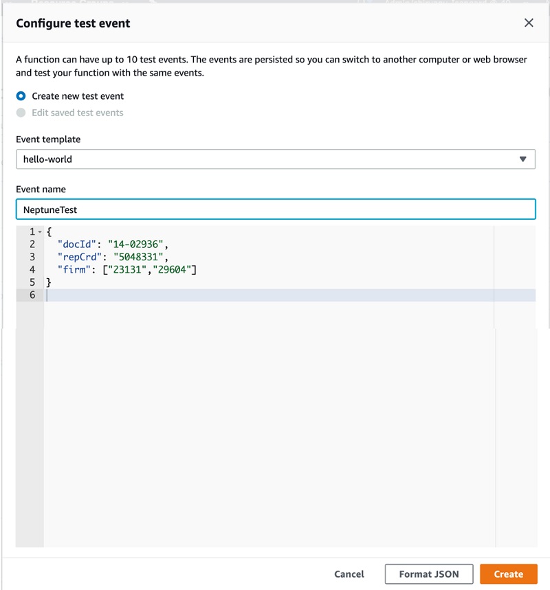
- In the Configure test event page, choose Create new test event.
- For Event template, choose the default Hello World
- For Event name, enter a name and note the following sample event template:
{
  "docId": "14-02936",
  "repCrd": "5048331",
  "firm": ["23131","29604"]
}
- Choose Create.
- Choose Test.
Each user can create up to 10 test events per function. Those test events aren’t available to other users.
Lambda runs your function on your behalf. The handler in your Lambda function receives and processes the sample event.
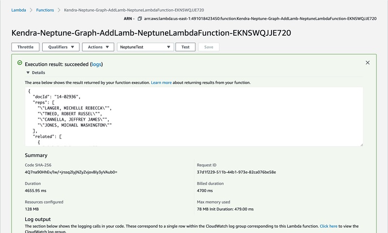
- After the function runs successfully, view the results on the Lambda console.
The results have the following sections:
- Execution result – Shows the run status as succeeded and also shows the function run results, returned by the return statement.
- Summary – Shows the key information reported in the Log output section (the
REPORT line in the run log).
- Log output – Shows the log Lambda generates for each run. These are the logs written to CloudWatch by the Lambda function. The Lambda console shows these logs for your convenience. The Click here link shows the logs on the CloudWatch console. The function then adds logs to CloudWatch in the log group that corresponds to the Lambda function.
Developing the web app
In this section, we develop a web app with a search interface to search the documents. We use AWS Cloud9 as our integrated development environment (IDE) and Amplify to build and deploy the web app.
AWS Cloud9 is a cloud-based IDE that lets you write, run, and debug your code with just a browser. It includes a code editor, debugger, and a terminal. AWS Cloud9 comes prepackaged with essential tools for popular programming languages, including JavaScript, Python, PHP, and more, so you don’t need to install files or configure your development machine to start new projects.
The AWS Cloud9 workspace should be built by an IAM user with administrator privileges, not the root account user. Please ensure you’re logged in as an IAM user, not the root account user.
Ad blockers, JavaScript disablers, and tracking blockers should be disabled for the AWS Cloud9 domain, otherwise connecting to the workspace might be impacted.
Creating a new environment
To create your environment, complete the following steps:
- On the AWS Cloud9 console, make sure you’re using one of the following Regions:
- US East (N. Virginia)
- US West (Oregon)
- Asia Pacific (Singapore)
- Europe (Ireland)
- Choose Create environment.
- Name the environment
kendrapoc.
- Choose Next step.
- Choose Create a new instance for environment (EC2) and choose small.
- Leave all the environment settings as their defaults and choose Next step.
- Choose Create environment.
Preparing the environment
To prepare your environment, make sure you’re in the default directory in an AWS Cloud9 terminal window (~/environment) before completing the following steps:
- Enter the following code to download the code for the Amazon Kendra sample app and extract it in a temporary directory:
mkdir tmp
cd tmp
aws s3 cp s3://aws-ml-blog/artifacts/Incorporating-your-enterprise-knowledge-graph-into-Amazon-Kendra/kendra-graph-blog-data/kendrasgraphsampleui.zip .
unzip kendrasgraphsampleui.zip
rm kendrasgraphsampleui.zip
cd ..
- We build our app in ReactJS with the following code:
echo fs.inotify.max_user_watches=524288 | sudo tee -a /etc/sysctl.conf && sudo sysctl -p
npx create-react-app kendra-poc
- Change the working directory to
kendra-poc and ensure that you’re in the /home/ec2-
user/environment/kendra-poc directory:
- Install a few prerequisites with the following code:
npm install --save node-sass typescript bootstrap react-bootstrap @types/lodash aws-sdk
npm install --save semantic-ui-react
npm install aws-amplify @aws-amplify/ui-react
npm install -g @aws-amplify/cli
- Copy the source code to the src directory:
cp -r ../tmp/kendrasgraphsampleui/* src/
Initializing Amplify
To initialize Amplify, complete the following steps:
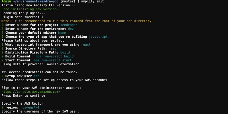
- On the command line, in the kendra-poc directory, enter the following code:
- Choose Enter.
- Accept the default project name
kendrapoc.
- Enter dev for the environment name.
- Choose None for the default editor (we use AWS Cloud9).
- Choose JavaScript and React when prompted.
- Accept the default values for paths and build commands.
- Choose the default profile when prompted.
Your run should look like the following screenshot.
Adding authentication
To add authentication to the app, complete the following steps:
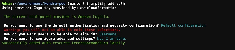
- Enter the following code:
- Choose Default Configuration when asked if you want to use the default authentication and security configuration.
- Choose Username when asked how you want users to sign in.
- Choose No, I am done. when asked about advanced settings.
This session should look like the following screenshot.
- To create these changes in the cloud, enter:
- Confirm you want Amplify to make changes in the cloud for you.
Provisioning takes a few minutes to complete. The Amplify CLI takes care of provisioning the appropriate cloud resources and updates src/aws-exports.js with all the configuration data we need to use the cloud resources in our app.
Amazon Cognito lets you add user sign-up, sign-in, and access control to your web and mobile apps quickly and easily. We made a user pool, which is a secure user directory that lets our users sign in with the user name and password pair they create during registration. Amazon Cognito (and the Amplify CLI) also supports configuring sign-in with social identity providers, such as Facebook, Google, and Amazon, and enterprise identity providers via SAML 2.0. For more information, see Amazon Cognito Developer and Amplify Authentication documentations
Configuring an IAM role for authenticated users
To configure your IAM role for authenticated users, complete the following steps:
- In the AWS Cloud9 IDE, in the left panel, browse to the file
kendra-poc/amplify/team-provider-info.json and open it (double-click).
- Note the value of
AuthRoleName.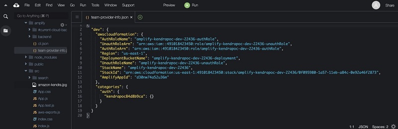
- On the IAM console, choose Roles.
- Search for the
AuthRole using the value from the previous step and open that role.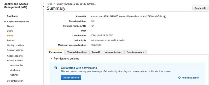
- Choose Add inline policy.
- Choose JSON and replace the contents with the following policy. Replace
enterprise-search-poc-ds-UNIQUE-SUFFIX with the name of the S3 bucket that is configured as the data source (leave the * after the bucket name, which allows the policy to access any object in the bucket). Replace ACCOUNT-NUMBER with the AWS account number and KENDRA-INDEX-ID with the index ID of your index.
{
    "Version": "2012-10-17",
    "Statement": [
        {
            "Sid": "VisualEditor0",
            "Effect": "Allow",
            "Action": "kendra:ListIndices",
            "Resource": "*"
        },
        {
            "Sid": "VisualEditor1",
            "Effect": "Allow",
            "Action": [
                "kendra:Query",
                "s3:ListBucket",
                "s3:GetObject",
                "kendra:ListFaqs",
                "kendra:ListDataSources",
                "kendra:DescribeIndex",
                "kendra:DescribeFaq",
                "kendra:DescribeDataSource"
            ],
            "Resource": [
                "arn:aws:s3:::enterprise-search-poc-ds-UNIQUE-SUFFIX*",
                "arn:aws:kendra:us-east-1:ACCOUNT-NUMBER:index/KENDRA-INDEX-ID"
            ]
        }
    ]
}
- Choose Review policy.
- Enter a policy name, such as
my-kendra-poc-policy.
- Choose Create policy.
- Browse back to the role and confirm that
my-kendra-poc-policy is present.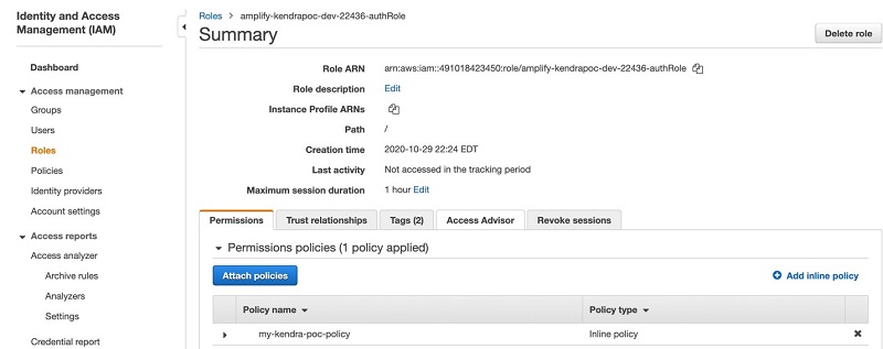
- Create a user (
poctester - customer) and add to the corresponding groups by entering the following at the command prompt:
USER_POOL_ID=`grep user_pools_id src/aws-exports.js| awk 'BEGIN {FS =""" } {print $4}'`
aws cognito-idp create-group --group-name customer --user-pool-id $USER_POOL_ID
aws cognito-idp admin-create-user --user-pool-id $USER_POOL_ID --username poctester --temporary-password AmazonKendra
aws cognito-idp admin-add-user-to-group --user-pool-id $USER_POOL_ID --username poctester --group-name customer
Configuring the application
You’re now ready to configure the application.
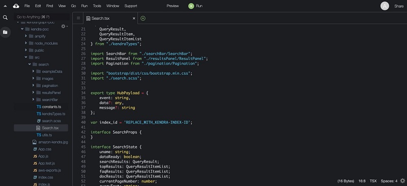
- In the AWS Cloud9 environment, browse to the file
kendra-poc/src/search/Search.tsx and open it for editing.
A new window opens.
- Replace REPLACE_WITH_KENDRA-INDEX-ID with your index ID.
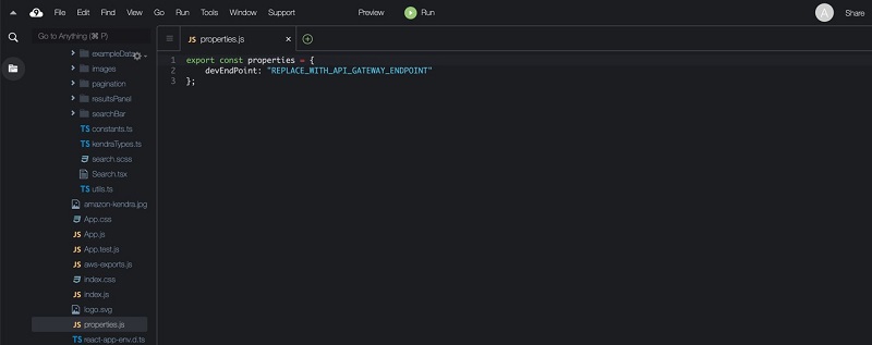
- In the AWS Cloud9 environment, browse to the file
kendra-poc/src/properties.js and open it for editing.
- In the new window that opens, replace REPLACE_WITH_API_GATEWAY_ENDPOINT with the PI Gateway invoke URL value from earlier.
- Start the application in the AWS Cloud9 environment by entering the following code in the command window in the
~/environment/kendra-poc directory:
Compiling the code and starting takes a few minutes.
- Preview the running application by choosing Preview on the AWS Cloud9 menu bar.
- From the drop-down menu, choose Preview Running Application.
A new browser window opens.
- Log in with any of the users we configured earlier (
poctester) with the temporary password AmazonKendra.
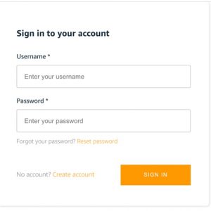
Amazon Cognito forces a password reset upon first login.
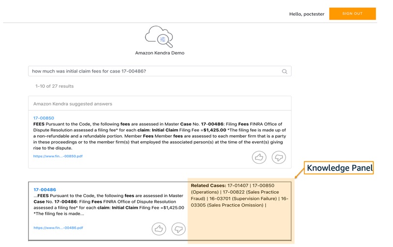
Using the application
Now we can try out the app we developed by making a few search queries, such as “how much was initial claim fees for case 17-00486?”
The following screenshot shows the Amazon Kendra results and the knowledge panel, which shows the related cases for each result. The knowledge panel details on the left is populated from the graph database and shows all the related cases for each search item.
Conclusion
This post demonstrated how to build a targeted and flexible cognitive search engine with a knowledge graph stored in Neptune and integrated with Amazon Kendra. You can enable rapid search for your documents and graph data using natural language, without any previous AI or ML experience. Finally, you can create an ensemble of other content types, including any combination of structured and unstructured documents, to make your archives indexable and searchable for harvesting knowledge and gaining insight. For more information about Amazon Kendra, see AWS re:Invent 2019 – Keynote with Andy Jassy on YouTube, Amazon Kendra FAQs, and What is Amazon Kendra?
About the Authors
 Dr. Yazdan Shirvany is all 12 AWS-certified Senior Solution Architect with deep experience in AI/ML, IOT and big data technologies including NLP, Knowledge Graph, applications reengineering, and optimizing software to leverage the cloud. Dr. Shirvany has 20+ scientific publications, and several issued patents in AI/ML field. Dr. Shirvany holds a M.S and Ph.D. in Computer Science from Chalmers University of Technology.
 Dipto Chakravarty is a leader in Amazon’s Alexa engineering group and heads up the Personal Mobility team in HQ2 utilizing AI, ML and IoT to solve local search analytics challenges. He has 12 patents issued to date and has authored two best-selling books on computer architecture and operating systems published by McGraw-Hill and Wiley. Dipto holds a B.S and M.S in Computer Science and Electrical Engineering from U. of Maryland, an EMBA from Wharton School, U. Penn, and a GMP from Harvard Business School.
 Mohit Mehta is a leader in the AWS Professional Services Organization with expertise in AI/ML and Big Data technologies. Mohit holds a M.S in Computer Science, all 12 AWS certifications, MBA from College of William and Mary and GMP from Michigan Ross School of Business.
Read More


 Kashif Imran is a Principal Solutions Architect at Amazon Web Services. He works with some of the largest AWS customers who are taking advantage of AI/ML to solve complex business problems. He provides technical guidance and design advice to implement computer vision applications at scale. His expertise spans application architecture, serverless, containers, NoSQL and machine learning.
 Peter M. O’Donnell is an AWS Principal Solutions Architect, specializing in security, risk, and compliance with the Strategic Accounts team. Formerly dedicated to a major US commercial bank customer, Peter now supports some of AWS’s largest and most complex strategic customers in security and security-related topics, including data protection, cryptography, incident response, and CISO engagement.
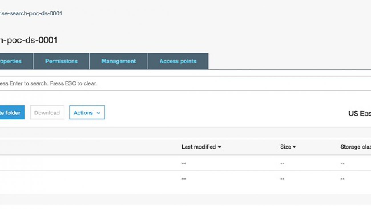


