AI models exceed human performance on public data sets; modified training and testing could help ensure that they aren’t exploiting short cuts.Read More

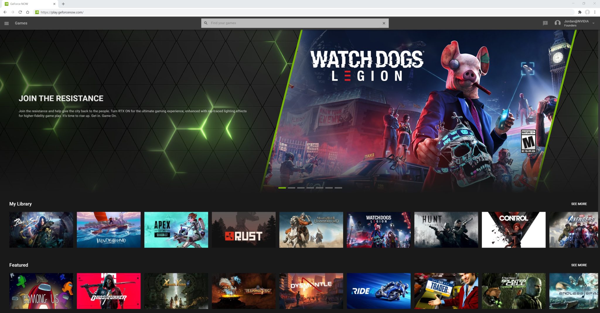
GeForce NOW Streaming Comes to iOS Safari
GeForce NOW transforms underpowered or incompatible hardware into high-performance GeForce gaming rigs.
Now, we’re bringing the world of PC gaming to iOS devices through Safari.
GeForce NOW is streaming on iOS Safari, in beta, starting today. That means more than 5 million GeForce NOW members can now access the latest experience by launching Safari from iPhone or iPad and visiting play.geforcenow.com.
Not a member? Get started by signing up for a Founders membership that offers beautifully ray-traced graphics on supported games, extended sessions lengths and front-of-the-line access. There’s also a free option for those who want to test the waters.
Right now is a great time to join. Founders memberships are available for $4.99/month or lock in an even better rate with a six-month Founders membership for $24.95.
All new GeForce RTX 30 Series GPUs come bundled with a GeForce NOW Founders membership, available to existing or new members.
Once logged in, you’re only a couple clicks away from streaming a massive catalog of the latest and most played PC games. Instantly jump into your games, like Assassin’s Creed Valhalla, Destiny 2 Beyond Light, Shadow of the Tomb Raider and more. Founders members can also play titles like Watch Dogs: Legion with RTX ON and NVIDIA DLSS, even on their iPhone or iPad.
GeForce NOW on iOS Safari requires a gamepad — keyboard and mouse-only games aren’t available due to hardware limitations. For the best experience, you’ll want to use a GeForce NOW Recommended gamepad, like the Razer Kishi.
Fortnite, Coming Soon
Alongside the amazing team at Epic Games, we’re working to enable a touch-friendly version of Fortnite, which will delay availability of the game. While the GeForce NOW library is best experienced on mobile with a gamepad, touch is how over 100 million Fortnite gamers have built, battled and danced their way to Victory Royale.
We’re looking forward to delivering a cloud-streaming Fortnite mobile experience powered by GeForce NOW. Members can look for the game on iOS Safari soon.
More Games, More Game Stores
When you fire up your favorite game, you’re playing it instantly — that’s what it means to be Game Ready on GeForce NOW. The experience has been optimized for cloud gaming and includes Game Ready Driver performance improvements.

NVIDIA manages the game updates and patches, letting you play the games you own at 1080p, 60FPS across nearly all of your devices. And when a game supports RTX, Founders members can play with beautifully ray-traced graphics and DLSS 2.0 for improved graphics fidelity.
PC games become playable across a wider range of hardware, removing the barriers across platforms. With the recent release of Among Us, Mac and Chromebook owners can now experience the viral sensation, just like PC gamers. Android owners can play the newest titles even when they’re away from their rig.
More than 750 PC games are now Game Ready on GeForce NOW, with weekly additions that continue to expand the library.
Coming soon, GeForce NOW will connect with GOG, giving members access to even more games in their library. The first GOG.com games that we anticipate supporting are CD PROJEKT RED’s Cyberpunk 2077 and The Witcher 3: Wild Hunt.
The GeForce-Powered Cloud
Founders members have turned RTX ON for beautifully ray-traced graphics, and can run games with even higher fidelity thanks to DLSS. That’s the power to play that only a GeForce-powered cloud gaming service can deliver.
The advantages also extend to improving quality of service. By developing both the hardware and software streaming solutions, we’re able to easily integrate new GeForce technologies that reduce latency on good networks, and improve fidelity on poor networks.
These improvements will continue over time, with some optimizations already available and being felt by GeForce NOW members today.
Chrome Wasn’t Built in a Day
The first webRTC client running GeForce NOW was the Chromebook beta in August. In the months since, we’ve seen over 10 percent of gameplay in the Chrome web-based client.
Soon we’ll bring that experience to more Chrome platforms, including Linux, PC, Mac and Android. Stay tuned for updates as we approach a full launch early next year.
Expanding to New Regions
The GeForce NOW Alliance continues to spread cloud gaming across the globe. The alliance is currently made up of LG U+ and KDDI in Korea, SoftBank in Japan, GFN.RU in Russia and Taiwan Mobile, which launched out of beta on Nov. 7.
In the weeks ahead, Zain KSA, the leading 5G telecom operator in Saudi Arabia, will launch its GeForce NOW beta for gamers, expanding cloud gaming into another new region.
More games. More platforms. Legendary GeForce performance. And now streaming on iOS Safari. That’s the power to play that only GeForce NOW can deliver.
The post GeForce NOW Streaming Comes to iOS Safari appeared first on The Official NVIDIA Blog.
How Rajeev Rastogi’s machine learning team in India develops innovations for customers worldwide
Team works to address the needs of 600 million people online who together speak more than 22 Indian languages with over 19,500 dialects.Read More

Using Model Card Toolkit for TF Model Transparency
 Posted by Karan Shukla, Software Engineer, Google Research
Machine learning (ML) model transparency is important across a wide variety of domains that impact peoples’ lives, from healthcare to personal finance to employment. At Google, this desire for transparency led us to develop Model Cards, a framework for transparent reporting on ML model performance, provenance, ethical considerations and more. It can be time consuming, however, to compile the information necessary to create a useful Model Card. To address this, we recently announced the open-source launch of Model Card Toolkit (MCT), a collection of tools that supports ML developers in compiling the information that goes into a Model Card.
The toolkit consists of:
- A JSON schema, which specifies the fields to include in the Model Card
- A ModelCard data API to represent an instance of the JSON schema and visualize it as a Model Card
- A component that uses the model provenance information stored with ML Metadata (MLMD) to automatically populate the JSON with relevant information
We wanted the toolkit to be modular so that Model Card creators can still leverage the JSON schema and ModelCard data API even if their modeling environment is not integrated with MLMD. In this post, we’ll show you how you can use these components to create a Model Card for a Keras MobileNetV2 model trained on ImageNet and fine-tuned on the cats_vs_dogs dataset available in TensorFlow Datasets (TFDS). While this model and use case may be trivial from a transparency standpoint, it allows us to easily demonstrate the components of MCT.
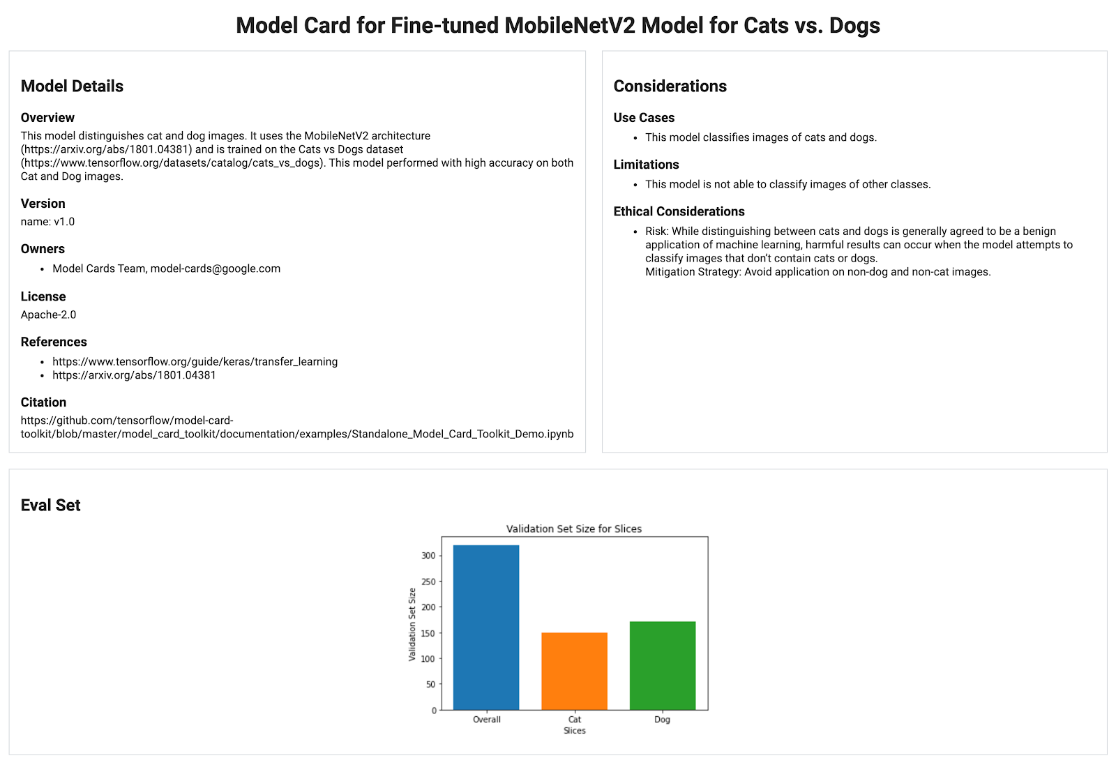
|
| An example Model Card. Click here for a larger version. |
Model Card Toolkit Walkthrough
You can follow along and run the code yourself in the Colab notebook. In this walkthrough, we’ll include some additional information about the considerations you’ll want to keep in mind while using the toolkit.
We begin by installing the Model Card Toolkit.
!pip install 'model-card-toolkit>=0.1.1,
Now, we load both the MobileNetV2 model and the weights generated by fine-tuning the model on the cats_vs_dogs dataset. For more information on how we fine-tuned our model, you can see the TensorFlow tutorial on the topic.
URL = 'https://storage.googleapis.com/cats_vs_dogs_model/cats_vs_dogs_model.zip'
BASE_PATH = tempfile.mkdtemp()
ZIP_PATH = os.path.join(BASE_PATH, 'cats_vs_dogs_model.zip')
MODEL_PATH = os.path.join(BASE_PATH,'cats_vs_dogs_model')

r = requests.get(URL, allow_redirects=True)
open(ZIP_PATH, 'wb').write(r.content)

with zipfile.ZipFile(ZIP_PATH, 'r') as zip_ref:
    zip_ref.extractall(BASE_PATH)

model = tf.keras.models.load_model(MODEL_PATH)
We also calculate the number of examples, storing it to the “examples” object, and the accuracy scores, disaggregated across class. We’ll use both accuracy and examples later to build graphs to display in our Model Card.
examples = cats_vs_dogs.get_data()
accuracy = compute_accuracy(examples['combined'])
cat_accuracy = compute_accuracy(examples['cat'])
dog_accuracy = compute_accuracy(examples['dog'])
Next, we’ll use the Model Card Toolkit to create our Model Card. The first step is to initialize a ModelCardToolkit object, which maintains assets including a Model Card JSON file and Model Card document. Call ModelCardToolkit.scaffold_assets() to generate these assets and return a ModelCard object.
model_card_dir = tempfile.mkdtemp()
mct = ModelCardToolkit(model_card_dir)
model_card = mct.scaffold_assets()
We then populate the Model Card’s fields. First, we’ll fill in the model_card.model_details section, which contains basic metadata fields.
We begin by specifying the model’s name, writing a brief description of the model in the overview section.
model_card.model_details.name = 'Fine-tuned MobileNetV2 Model for Cat vs. Dogs'
model_card.model_details.overview = (
   'This model distinguishes cat and dog images. It uses the MobileNetV2 '
   'architecture (https://arxiv.org/abs/1801.04381) and is trained on the '
   'Cats vs Dogs dataset '
   '(https://www.tensorflow.org/datasets/catalog/cats_vs_dogs). This model '
   'performed with high accuracy on both Cat and Dog images.'
  )
We provide the model’s owners, version, and references.
model_card.model_details.owners = [
 {'name': 'Model Cards Team', 'contact': 'model-cards@google.com'}
]
model_card.model_details.version = {'name': 'v1.0', 'data': '08/28/2020'}
model_card.model_details.references = [
   'https://www.tensorflow.org/guide/keras/transfer_learning',
   'https://arxiv.org/abs/1801.04381',
  ]
Finally, we share the model’s license information, and a url that future users can cite if they choose to reuse the model in the citation section.
model_card.model_details.license = 'Apache-2.0'
model_card.model_details.citation = 'https://github.com/tensorflow/model-card-toolkit/blob/master/model_card_toolkit/documentation/examples/Standalone_Model_Card_Toolkit_Demo.ipynb'
The model_card.quantitative_analysis field contains information about a model's performance metrics. Here, we’ve created some synthetic performance metric values for a hypothetical model built on our dataset.
model_card.quantitative_analysis.performance_metrics = [
 {'type': 'accuracy', 'value': accuracy},
 {'type': 'accuracy', 'value': cat_accuracy, 'slice': 'cat'},
 {'type': 'accuracy', 'value': dog_accuracy, 'slice': 'Dog'},
]
model_card.considerations contains qualitative information about your model. In particular, we recommend including some, or all of the following information:
Use cases: What are the intended use cases for this model? This is pretty straightforward for our model:
model_card.considerations.use_cases = [
   'This model classifies images of cats and dogs.'
]
Limitations: What technical limitations should users keep in mind? What kinds of data cause your model to fail, or underperform? In our case, examples that are not dogs or cats will cause our model to fail, so we’ve acknowledged this:
model_card.considerations.limitations = [
   'This model is not able to classify images of other animals.'
]
Ethical considerations: What ethical considerations should users be aware of when deciding whether or not to use the model? In what contexts could the model raise ethical concerns? What steps did you take to mitigate ethical concerns?
model_card.considerations.ethical_considerations = [{
   'name':
       'While distinguishing between cats and dogs is generally agreed to be '
       'a benign application of machine learning, harmful results can occur '
       'when the model attempts to classify images that don’t contain cats or '
       'dogs.',
   'mitigation_strategy':
       'Avoid application on non-dog and non-cat images.'
}]
Lastly, you can include graphs in your Model Card. We recommend including graphs that reflect the distributions in both your training and evaluation datasets, as well as graphs of your model’s performance on evaluation data. model_card has sections for each of these:
model_card.model_parameters.data.train.graphicsfor training dataset statisticsmodel_card.model_parameters.data.eval.graphicsfor evaluation dataset statisticsmodel_card.quantitative_analysis.graphicsfor quantitative analysis of model performance
For this Model Card, we’ve included Matplotlib graphs of our validation set size and the model’s accuracy, both separated by class. Please visit the associated Colab if you’d like to see the Matplotlib code. If you are using ML Metadata, these graphs will be generated automatically (as demonstrated in this Colab). You can also use other visualization libraries, like Seaborn.
We add our graphs to our Model Card.
model_card.model_parameters.data.eval.graphics.collection = [
 {'name': 'Validation Set Size', 'image': validation_set_size_barchart},
]
model_card.quantitative_analysis.graphics.collection = [
 {'name': 'Accuracy', 'image': accuracy_barchart},
]
We’re finally ready to generate our Model Card! Let’s do that now. First we need to update the ModelCardToolkit object with the latest ModelCard.
mct.update_model_card_json(model_card)Lastly, we generate the Model Card document in the chosen output format.
# Generate a model card document in HTML (default)
html_doc = mct.export_format()

# Display the model card document in HTML
display.display(display.HTML(html_doc))


# Generate a model card document in Markdown
md_path = os.path.join(model_card_dir, 'template/md/default_template.md.jinja')
md_doc = mct.export_format(md_path, 'model_card.md')

# Display the model card document in Markdown
display.display(display.Markdown(md_doc))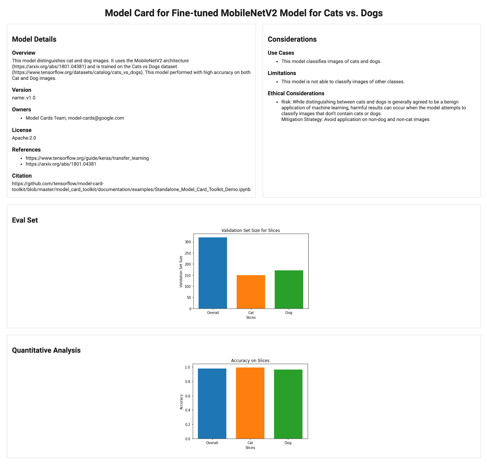
And we’ve generated our Model Card! It’s a good idea to review the end product with your direct team, as well as members who are further away from the project. In particular, we recommend reviewing the qualitative fields such as “ethical considerations” to ensure you’ve adequately captured all potential use cases and their potential consequences. Does your Model Card answer the questions that people from different backgrounds might have? Is the language accessible to a developer? What about a policy maker, or a downstream user who might interact with the model? In the future, we hope to offer Model Card creators more guidance that they can use to help answer these questions and provide more thorough instructions on how to fill out the considerations fields.
Have questions? Have Model Cards to share? Let us know at model-cards@google.com!
Acknowledgements
Huanming Fang, Hui Miao, Karan Shukla, Dan Nanas, Catherina Xu, Christina Greer, Neoklis Polyzotis, Tulsee Doshi, Tiffany Deng, Margaret Mitchell, Timnit Gebru, Andrew Zaldivar, Mahima Pushkarna, Meena Natarajan, Roy Kim, Parker Barnes, Tom Murray, Susanna Ricco, Lucy Vasserman, and Simone Wu
Using Transformers to create music in AWS DeepComposer Music studio
AWS DeepComposer provides a creative and hands-on experience for learning generative AI and machine learning (ML). We recently launched a Transformer-based model that iteratively extends your input melody up to 20 seconds. This newly created extension will use the style and musical motifs found in your input melody and create additional notes that sound like they’ve come from your input melody. In this post, we show you how the Transformer model extends the duration of your existing compositions. You can create new and interesting musical scores by using various parameters, including the Edit melody feature.
Introduction to Transformers
The Transformer is a recent deep learning model for use with sequential data such as text, time series, music, and genomes. Whereas older sequence models such as recurrent neural networks (RNNs) or long short-term memory networks (LSTMs) process data sequentially, the Transformer processes data in parallel. This allows them to process massive amounts of available training data by using powerful GPU-based compute resources.
Furthermore, traditional RNNs and LSTMs can have difficulty modeling the long-term dependencies of a sequence because they can forget earlier parts of the sequence. Transformers use an attention mechanism to overcome this memory shortcoming by directing each step of the output sequence to pay “attention” to relevant parts of the input sequence. For example, when a Transformer-based conversational AI model is asked “How is the weather now?” and the model replies “It is warm and sunny today,” the attention mechanism guides the model to focus on the word “weather” when answering with “warm” and “sunny,” and to focus on “now” when answering with “today.” This is different from traditional RNNs and LSTMs, which process sentences from left to right and forget the context of each word as the distance between the words increases.
Training a Transformer model to generate music
To work with musical datasets, the first step is to convert the data into a sequence of tokens. Each token represents a distinct musical event in the score. A token might represent something like the timestamp for when a note is struck, or the pitch of a note. The relationship between these tokens to musical notes is similar to the relationship between words in a sentence or paragraph. Tokens in music can represent notes or other musical features just like how tokens in language can represent words or punctuation. This differs from previous models supported by AWS DeepComposer such as GAN and AR-CNN, which treat music generation like an image generation problem.
These sequences of tokens are then used to train the Transformer model. During training, the model attempts to learn a distribution that matches the underlying distribution of the training dataset. During inference, the model generates a sequence of tokens by sampling from the distribution learned during training. The new musical score is created by turning the sequence of tokens back into music. Music Transformer and MuseNet are examples of other algorithms that use the Transformer architecture for music generation.
In AWS DeepComposer, we use the TransformerXL architecture to generate music because it’s capable of capturing long-term dependencies that are 4.5 times longer than a traditional Transformer. Furthermore, it has been shown to be 18 times faster than a traditional Transformer during inference. This means that AWS DeepComposer can provide you with higher quality musical compositions at lower latency when generating new compositions.
Extending your input melody using AWS DeepComposer
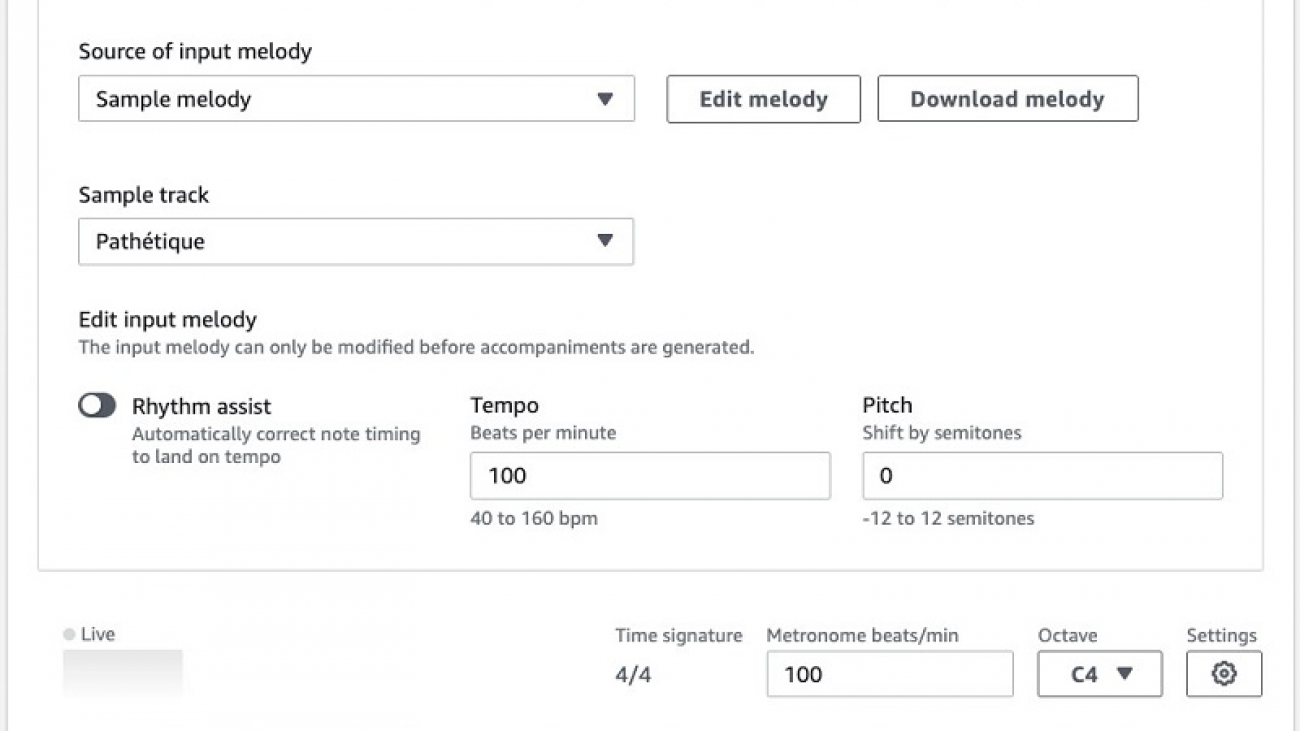
The Transformers technique extends your input melody by up to 20 seconds. The following screenshot shows the view of your input melody on the AWS DeepComposer console.
![]()
To extend your input melody, complete the following steps:
- On the AWS DeepComposer console, in the navigation pane, choose Music studio.
- Choose the arrow next to Input melody to expand that section.
- For Sample track, choose a melody specifically recommended for the Transformers technique.
These options represent the kinds of complex classical-genre melodies that will work best with the Transformer technique. You can also import a MIDI file or create your own melody using a MIDI keyboard.
- Under Generative AI technique, for Model parameters, choose Transformers.
The available model, TransformerXLClassical, is preselected.
- Under Advanced parameters, for Model parameters, you have seven parameters that you can adjust (more details about these parameters are provided in the next section of this post).
- Choose Extend input melody.
- To listen to your new composition, choose Play (►).
This model works by extending your input melody by up to 20 seconds.
- After performing inference, you can use the Edit melody tool to add or remove notes, or change the pitch or the length of notes in the track generated.
- You can repeat these steps to create compositions up to 2 minutes long.
The following compositions were created using the TransformersXLClassical model in AWS DeepComposer:
Beethoven:
Mozart:
Bach:
In the next section of this post, we look at how different inference parameters affect your output and how we can effectively use these parameters to create interesting and diverse music.
Configuring the advanced parameters for Transformers
In AWS DeepComposer Music studio, you can choose from seven different Advanced parameters that can be used to change how your extended melody is created:
- Sampling technique and sampling threshold
- Creative risk
- Input duration
- Track extension duration
- Maximum rest time
- Maximum note length
Sampling technique and sampling threshold
You have three sampling techniques to choose from: TopK, Nucleus, and Random. You can also set the Sampling threshold value for your chosen technique. We first discuss each technique and provide some examples of how it affects the output below.
TopK sampling
When you choose the TopK sampling technique, the model chooses the K-tokens that have the highest probability of occurring. To set the value for K, change the Sampling threshold.
If your sampling threshold is set high, the number of available tokens (K) is large. A large number of available tokens means the model can choose from a wider variety of musical tokens. In your extended melody, this means the generated notes are likely to be more diverse, but it comes at the cost of potentially creating less coherent music.
On the other hand, if you choose a threshold value that is too low, the model is limited to choosing from a smaller set of tokens (that the model believes has a higher probability of being correct). In your extended melody, you might notice less musical diversity and more repetitive results.
Nucleus sampling
At a high level, Nucleus sampling is very similar to TopK. Setting a higher sampling threshold allows for more diversity at the cost of coherence or consistency. There is a subtle difference between the two approaches. Nucleus sampling chooses the top probability tokens that sum up to the value set for the sampling threshold. We do this by sorting the probabilities from greatest to least, and calculating a cumulative sum for each token.
For example, we might have six musical tokens with the probabilities {0.3, 0.3, 0.2, 0.1, 0.05, 0.05}. If we choose TopK with a sampling threshold equal to 0.5, we choose three tokens (six total musical tokens * 0.5). Then we sample between the tokens with probabilities equal to 0.3, 0.3, and 0.2. If we choose Nucleus sampling with a 0.5 sampling threshold, we only sample between two tokens {0.3, 0.3} as the cumulative probability (0.6) exceeds the threshold (0.5).
Random sampling
Random sampling is the most basic sampling technique. With random sampling, the model is free to sample between all the available tokens and is “randomly” sampled from the output distribution. The output of this sampling technique is identical to that of TopK or Nucleus sampling when the sampling threshold is set to 1. The following are some audio clips generated using different sampling thresholds paired with the TopK sampling threshold.
The following audio uses TopK and a Sampling threshold equal to 0.1:
Notice how the notes quickly start to form a pattern.
The following audio uses TopK and a Sampling threshold equal to 0.9:
You can decide which one sounds better, but did you hear the difference?
The notes are very diverse, but as a whole the notes lose coherence and sound somewhat random at times. This general trend holds for Nucleus sampling as well, but the results differ from TopK depending on the shape of the output distribution. Play around and see for yourself!
Creative risk
Creative risk is a parameter used to control the randomness of predictions. A low creative risk makes the model more confident but also more conservative in its samples (it’s less likely to sample from unlikely candidate tokens). On the other hand, a high creative risk produces a softer (flatter) probability distribution over the list of musical tokens, so the model takes more risks in its samples (it’s more likely to sample from unlikely candidate tokens), resulting in more diversity and probably more mistakes. Mistakes might include creating longer or shorter notes, longer or shorter periods of rest in the generated melody, or adding wrong notes to the generated melody.
Input duration
This parameter tells the model what portion of the input melody to use during inference. The portion used is defined as the number of seconds selected counting backwards from the end of the input track. When extending the melody, the model conditions the output it generates based on the portion of the input melody you provide. For example, if you choose 5 seconds as the input duration, the model only uses the last 5 seconds of the input melody for conditioning and ignores the remaining portion when performing inference. The following audio clips were generated using different input durations.
The following audio has an input duration of 5 seconds:
The following audio has an input duration of 30 seconds:
The output conditioned on 30 seconds of input draws more inspiration from the input melody.
Track extension duration
When extending the melody, the Transformer continuously generates tokens until the generated portion reaches the track extension duration you have selected. The reason the model sometimes generates less than the value you selected is because the model generates values in terms of tokens, not time. Tokens, however, can represent different lengths of the time. For example, a token could represent a note duration of 0.1 seconds or 1 second depending on what the model thinks is appropriate. That token, however, takes the same amount of run time for the model to generate. Because the model can generate hundreds of tokens, this difference adds up. To make sure the model doesn’t have extreme runtime latencies, sometimes the model stops before generating your entire output.
Maximum rest time
During inference, the Transformers model can create musical artifacts. Changing the value of maximum rest time limits the periods of silence, in seconds, the model can generate while performing inference.
Maximum note length
Changing the value of maximum note length limits the amount of time a single note can be held for while performing inference. The following audio clips are some example tracks generated using different maximum rest time and maximum note length.
In the first example audio, we set the maximum note length to 10 seconds.
In the second sample, we set it to 1 second, but set the maximum rest period to 11 seconds.
In the third sample, we set the maximum note length to 1 second and maximum rest period to 2 seconds.
The first sample contains extremely long notes. The second sample doesn’t contain long notes, but contains many missing gaps in the music. On the other hand, the third sample contains both shorter notes and shorter gaps.
Creating compositions using different AWS DeepComposer techniques
What’s great about AWS DeepComposer is that you can mix and match the new Transformers technique with the other techniques found in AWS DeepComposer, such as the AR-CNN and GAN techniques.
To create a sample, we completed the following steps:
- Choose the sample melody Pathétique.
- Use the Transformers technique to extend the melody.
For this track, we extended the melody to 11 bars. Transformers tries to extend the melody up to the value you choose for the extension duration.
- The AR-CNN and GAN techniques only work with eight bars of input, so we use the Edit melody feature to cut the track down to eight bars.
![]()
- Use the AR-CNN technique to fill in notes and enhance the melody.
For this post, we set Sampling iterations equal to 100.
- We use the GAN technique, paired with the MuseGAN algorithm and the Rock model, to generate accompaniments.
The following audio is our final output:
We think the output sounds pretty impressive. What do you think? Play around and see what kind of composition you can create yourself!
Conclusion
You’ve now learned about the Transformer model and how AWS DeepComposer uses it to extend your input melody. You can also better understand how each parameter for the Transformers technique can affect the characteristics of your composition.
To continue exploring AWS DeepComposer, consider some of the following:
- Choose a different input melody. You can try importing a track or recording your own.
- Use the Edit melody feature to assist your AI or correct mistakes.
- Try feeding the output of the AR-CNN model into the Transformers model.
- Iteratively extend your melody to create a musical composition up to 2 minutes long.
Although you don’t need a physical device to experiment with AWS DeepComposer, you can take advantage of a limited-time offer and purchase the AWS DeepComposer keyboard at a special price of $79.20 (20% off) on Amazon.com. The pricing includes the keyboard and a 3-month free trial of AWS DeepComposer.
We’re excited for you to try out various combinations to generate your creative musical piece. Start composing in the AWS DeepComposer Music Studio now!
About the Authors
 Rahul Suresh is an Engineering Manager with the AWS AI org, where he has been working on AI based products for making machine learning accessible for all developers. Prior to joining AWS, Rahul was a Senior Software Developer at Amazon Devices and helped launch highly successful smart home products. Rahul is passionate about building machine learning systems at scale and is always looking for getting these advanced technologies in the hands of customers. In addition to his professional career, Rahul is an avid reader and a history buff.

Wayne Chi is a ML Engineer and AI Researcher at AWS. He works on researching interesting Machine Learning problems to teach new developers and then bringing those ideas into production. Prior to joining AWS he was a Software Engineer and AI Researcher at JPL, NASA where he worked on AI Planning and Scheduling systems for the Mars 2020 Rover (Perseverance). In his spare time he enjoys playing tennis, watching movies, and learning more about AI.
 Liang Li is an AI Researcher at AWS, where she works on AI based products to bring new cutting-edge ideas about Deep Learning to teach developers. Prior to joining AWS, Liang graduated from the University of Tennessee Knoxville with a Ph. D in EE, and she has been focusing on ML projects since graduation. In her spare time, she enjoys cooking and hiking.
 Suri Yaddanapudi is an AI Researcher and ML Engineer at AWS. He works on researching and implementing modern machine learning algorithms across different domains and teaching them to customers in a fun way. Prior to joining AWS, Suri graduated with his Ph.D. degree from University of Cincinnati and his thesis was focused on implementing AI techniques to Drug Repurposing. In his spare time, he enjoys reading, watching anime and playing futsal.

Aashiq Muhamed is an AI Researcher and ML Engineer at AWS. He believes that AI can change the world and that democratizing AI is key to making this happen. At AWS, he works on creating meaningful AI products and translating ideas from academia into industry. Prior to joining AWS, he was a graduate student at Stanford where he worked on model reduction in robotics, learning and control. In his spare time he enjoys playing the violin and thinking about healthcare on MARS.

Patrick L. Cavins is a Programmer Writer for DeepComposer and DeepLens. Previously, he worked in radiochemistry using isotopically labelled compounds to study how plants communicate. In his spare time, he enjoys skiing, playing the piano, and writing.

Maryam Rezapoor is a Senior Product Manager with AWS AI Devices team. As a former biomedical researcher and entrepreneur, she finds her passion in working backward from customers’ needs to create new impactful solutions. Outside of work, she enjoys hiking, photography, and gardening.

Accelerating TensorFlow Performance on Mac
 Posted by Pankaj Kanwar and Fred Alcober
With TensorFlow 2, best-in-class training performance on a variety of different platforms, devices and hardware enables developers, engineers, and researchers to work on their preferred platform. TensorFlow users on Intel Macs or Macs powered by Apple’s new M1 chip can now take advantage of accelerated training using Apple’s Mac-optimized version of TensorFlow 2.4 and the new ML Compute framework. These improvements, combined with the ability of Apple developers being able to execute TensorFlow on iOS through TensorFlow Lite, continue to showcase TensorFlow’s breadth and depth in supporting high-performance ML execution on Apple hardware.
Performance on the Mac with ML Compute
The Mac has long been a popular platform for developers, engineers, and researchers. With Apple’s announcement last week, featuring an updated lineup of Macs that contain the new M1 chip, Apple’s Mac-optimized version of TensorFlow 2.4 leverages the full power of the Mac with a huge jump in performance.
ML Compute, Apple’s new framework that powers training for TensorFlow models right on the Mac, now lets you take advantage of accelerated CPU and GPU training on both M1- and Intel-powered Macs.
For example, the M1 chip contains a powerful new 8-Core CPU and up to 8-core GPU that are optimized for ML training tasks right on the Mac. In the graphs below, you can see how Mac-optimized TensorFlow 2.4 can deliver huge performance increases on both M1- and Intel-powered Macs with popular models.
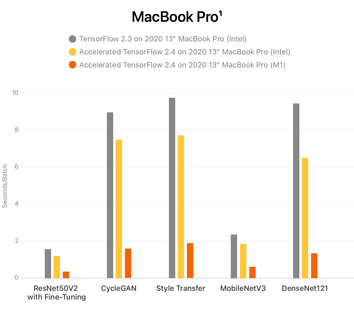 |
| Training impact on common models using ML Compute on M1- and Intel-powered 13-inch MacBook Pro are shown in seconds per batch, with lower numbers indicating faster training time. |
 |
| Training impact on common models using ML Compute on the Intel-powered 2019 Mac Pro are shown in seconds per batch, with lower numbers indicating faster training time. |
Getting Started with Mac-optimized TensorFlow
Users do not need to make any changes to their existing TensorFlow scripts to use ML Compute as a backend for TensorFlow and TensorFlow Addons.
To get started, visit Apple’s GitHub repo for instructions to download and install the Mac-optimized TensorFlow 2.4 fork.
In the near future, we’ll be making updates like this even easier for users to get these performance numbers by integrating the forked version into the TensorFlow master branch.
You can learn more about the ML Compute framework on Apple’s Machine Learning website.
Footnotes:
- Testing conducted by Apple in October and November 2020 using a preproduction 13-inch MacBook Pro system with Apple M1 chip, 16GB of RAM, and 256GB SSD, as well as a production 1.7GHz quad-core Intel Core i7-based 13-inch MacBook Pro system with Intel Iris Plus Graphics 645, 16GB of RAM, and 2TB SSD. Tested with prerelease macOS Big Sur, TensorFlow 2.3, prerelease TensorFlow 2.4, ResNet50V2 with fine-tuning, CycleGAN, Style Transfer, MobileNetV3, and DenseNet121. Performance tests are conducted using specific computer systems and reflect the approximate performance of MacBook Pro.
- Testing conducted by Apple in October and November 2020 using a production 3.2GHz 16-core Intel Xeon W-based Mac Pro system with 32GB of RAM, AMD Radeon Pro Vega II Duo graphics with 64GB of HBM2, and 256GB SSD. Tested with prerelease macOS Big Sur, TensorFlow 2.3, prerelease TensorFlow 2.4, ResNet50V2 with fine-tuning, CycleGAN, Style Transfer, MobileNetV3, and DenseNet121. Performance tests are conducted using specific computer systems and reflect the approximate performance of Mac Pro.

Haptics with Input: Using Linear Resonant Actuators for Sensing
Posted by Artem Dementyev, Hardware Engineer, Google Research
As wearables and handheld devices decrease in size, haptics become an increasingly vital channel for feedback, be it through silent alerts or a subtle “click” sensation when pressing buttons on a touch screen. Haptic feedback, ubiquitous in nearly all wearable devices and mobile phones, is commonly enabled by a linear resonant actuator (LRA), a small linear motor that leverages resonance to provide a strong haptic signal in a small package. However, the touch and pressure sensing needed to activate the haptic feedback tend to depend on additional, separate hardware which increases the price, size and complexity of the system.
In “Haptics with Input: Back-EMF in Linear Resonant Actuators to Enable Touch, Pressure and Environmental Awareness”, presented at ACM UIST 2020, we demonstrate that widely available LRAs can sense a wide range of external information, such as touch, tap and pressure, in addition to being able to relay information about contact with the skin, objects and surfaces. We achieve this with off-the-shelf LRAs by multiplexing the actuation with short pulses of custom waveforms that are designed to enable sensing using the back-EMF voltage. We demonstrate the potential of this approach to enable expressive discrete buttons and vibrotactile interfaces and show how the approach could bring rich sensing opportunities to integrated haptics modules in mobile devices, increasing sensing capabilities with fewer components. Our technique is potentially compatible with many existing LRA drivers, as they already employ back-EMF sensing for autotuning of the vibration frequency.
 |
| Different off-the-shelf LRAs that work using this technique. |
Back-EMF Principle in an LRA
Inside the LRA enclosure is a magnet attached to a small mass, both moving freely on a spring. The magnet moves in response to the excitation voltage introduced by the voice coil. The motion of the oscillating mass produces a counter-electromotive force, or back-EMF, which is a voltage proportional to the rate of change of magnetic flux. A greater oscillation speed creates a larger back-EMF voltage, while a stationary mass generates zero back-EMF voltage.
 |
| Anatomy of the LRA. |
Active Back-EMF for Sensing
Touching or making contact with the LRA during vibration changes the velocity of the interior mass, as energy is dissipated into the contact object. This works well with soft materials that deform under pressure, such as the human body. A finger, for example, absorbs different amounts of energy depending on the contact force as it flattens against the LRA. By driving the LRA with small amounts of energy, we can measure this phenomenon using the back-EMF voltage. Because leveraging the back-EMF behavior for sensing is an active process, the key insight that enabled this work was the design of a custom, off-resonance driver waveform that allows continuous sensing while minimizing vibrations, sound and power consumption.
 |
| Touch and pressure sensing on the LRA. |
We measure back-EMF from the floating voltage between the two LRA leads, which requires disconnecting the motor driver briefly to avoid disturbances. While the driver is disconnected, the mass is still oscillating inside the LRA, producing an oscillating back-EMF voltage. Because commercial back-EMF sensing LRA drivers do not provide the raw data, we designed a custom circuit that is able to pick up and amplify small back-EMF voltage. We also generated custom drive pulses that minimize vibrations and energy consumption.
 |
| Simplified schematic of the LRA driver and the back-EMF measurement circuit for active sensing. |
 |
| After exciting the LRA with a short drive pulse, the back-EMF voltage fluctuates due to the continued oscillations of the mass on the spring (top, red line). The change in the back-EMF signal when subject to a finger press depends on the pressure applied (middle/bottom, green/blue lines). |
Applications
The behavior of the LRAs used in mobile phones is the same, whether they are on a table, on a soft surface, or hand held. This may cause problems, as a vibrating phone could slide off a glass table or emit loud and unnecessary vibrating sounds. Ideally, the LRA on a phone would automatically adjust based on its environment. We demonstrate our approach for sensing using the LRA back-EMF technique by wiring directly to a Pixel 4’s LRA, and then classifying whether the phone is held in hand, placed on a soft surface (foam), or placed on a table.
 |
| Sensing phone surroundings. |
We also present a prototype that demonstrates how LRAs could be used as combined input/output devices in portable electronics. We attached two LRAs, one on the left and one on the right side of a phone. The buttons provide tap, touch, and pressure sensing. They are also programmed to provide haptic feedback, once the touch is detected.
 |
| Pressure-sensitive side buttons. |
There are a number of wearable tactile aid devices, such as sleeves, vests, and bracelets. To transmit tactile feedback to the skin with consistent force, the tactor has to apply the right pressure; it can not be too loose or too tight. Currently, the typical way to do so is through manual adjustment, which can be inconsistent and lacks measurable feedback. We show how the LRA back-EMF technique can be used to continuously monitor the fit bracelet device and prompt the user if it’s too tight, too loose, or just right.
 |
| Fit sensing bracelet. |
Evaluating an LRA as a Sensor
The LRA works well as a pressure sensor, because it has a quadratic response to the force magnitude during touch. Our method works for all five off-the-shelf LRA types that we evaluated. Because the typical power consumption is only 4.27 mA, all-day sensing would only reduce the battery life of a Pixel 4 phone from 25 to 24 hours. The power consumption can be greatly reduced by using low-power amplifiers and employing active sensing only when needed, such as when the phone is active and interacting with the user.
 |
| Back-EMF voltage changes when pressure is applied with a finger. |
The challenge with active sensing is to minimize vibrations, so they are not perceptible when touching and do not produce audible sound. We optimize the active sensing to produce only 2 dB of sound and 0.45 m/s2 peak-to-peak acceleration, which is just barely perceptible by finger and is quiet, in contrast to the regular 8.49 m/s2 .
Future Work and Conclusion
To see the work presented here in action, please see the video below.
In the future, we plan to explore other sensing techniques, perhaps measuring the current could be an alternative approach. Also, using machine learning could potentially improve the sensing and provide more accurate classification of the complex back-EMF patterns. Our method could be developed further to enable closed-loop feedback with the actuator and sensor, which would allow the actuator to provide the same force, regardless of external conditions.
We believe that this work opens up new opportunities for leveraging existing ubiquitous hardware to provide rich interactions and closed-loop feedback haptic actuators.
Acknowledgments
This work was done by Artem Dementyev, Alex Olwal, and Richard Lyon. Thanks to Mathieu Le Goc and Thad Starner for feedback on the paper.

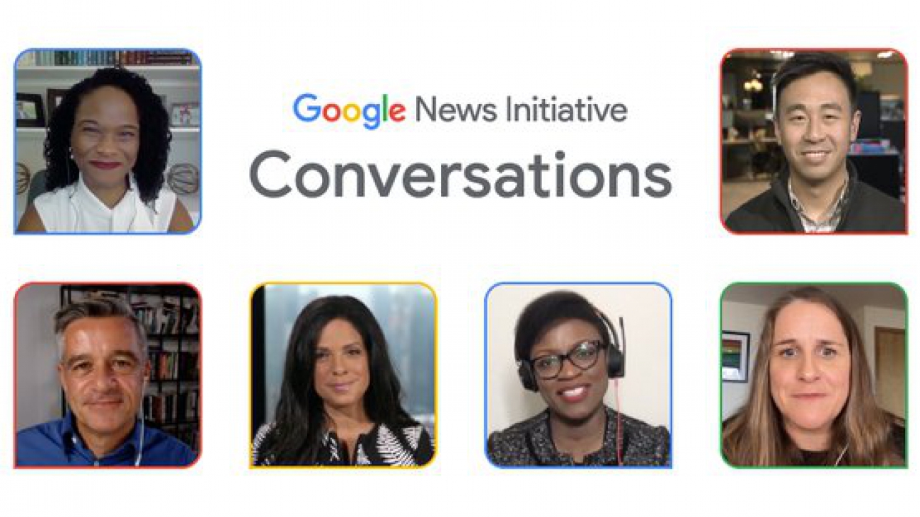
Introducing Google News Initiative Conversations
This year, the way many of us work has changed dramatically. We’ve gone from lunch meetings and large networking conferences to meeting virtually from our makeshift home offices. The COVID-19 pandemic has certainly upended a lot of this, but that doesn’t mean sharing ideas is on hold, too. That’s especially true for the Google News Initiative team; our commitment to helping journalism thrive is still just as strong.
That’s why we’ve launched Google News Initiative Conversations, a new video series in which we bring together industry experts and our partners from around the world to discuss the successes, challenges and opportunities facing the news industry. Since March 2018, the GNI has worked with more than 6,250 news partners in 118 countries, several of which are featured in the series.
Over the course of four episodes, we cover the themes of business sustainability, quality journalism, diversity, equity and inclusion and a look ahead to 2021 from a global perspective. Take a look at what the series has to offer:
Sustaining the News Industry, featuring:
Miki King, Chief Marketing Officer of the Washington Post
Gary Liu, CEO of the South China Morning Post
Tara Lajumoke, Managing Director of FT Strategies
Megan Brownlow and Simon Crerar talk about local journalism in Australia.

Quality Journalism, featuring:
Claire Wardle, U.S. Director, First Draft
Surabhi Malik and Syed Nazakat of FactShala India
Diversity, Equity, and Inclusion, featuring:
Soledad O’Brien, CEO of Soledad O’Brien Productions
Drew Christie, Chair of BCOMS – the Black Collective of Media in U.K. Sport
Bryan Pollard, Associate Director of Native American Journalists Association
Kalhan Rosenblatt, Youth and Internet Culture Reporter at NBC News
Tania Montalvo, General Editor at Animal Político, Mexico
Zack Weiner, President of Overtime

Innovation and the Future of News, featuring:
Brad Bender, VP of Product at Google interviewed by broadcaster Tina Daheley
Charlie Beckett, Professor in the Dept of Media and Communication at LSE
Agnes Stenborn, Responsible Data and AI Specialist
Christina Elmer, Editorial RnD at Der Spiegel

It’s uncertain when we’ll get to gather together in person again, but until then, we’ll continue learning, collaborating and innovating as we work towards a better future for news.

Rachel Malarich is planting a better future, tree by tree
Everyone has a tree story, Rachel Malarich says—and one of hers takes place on the limbs of a eucalyptus tree. Rachel and her cousins spent summers in central California climbing the 100-foot tall trees and hanging out between the waxy blue leaves—an experience she remembers as awe-inspiring.
Now, as Los Angeles first-ever City Forest Officer, Rachel’s work is shaping the tree stories that Angelenos will tell. “I want our communities to go to public spaces and feel that sense of awe,” she says. “That feeling that something was there before them, and it will be there after them…we have to bring that to our cities.”
Part of Rachel’s job is to help the City of Los Angeles reach an ambitious goal: to plant and maintain 90,000 trees by the end of 2021 and to keep planting trees at a rate of 20,000 per year after that. This goal is about more than planting trees, though: It’s about planting the seeds for social, economic and environmental equity. These trees, Rachel says, will help advance citywide sustainability and climate goals, beautify neighborhoods, improve air quality and create shade to combat rising street-level temperatures.
To make sure every tree has the most impact, Rachel and the City of Los Angeles use Tree Canopy Lab, a tool they helped build with Google that uses AI and aerial imagery to understand current tree cover density, also known as “tree canopy,” right down to street-level data. Tree inventory data, which is typically collected through on-site assessments, helps city officials know where to invest resources for maintaining, preserving and planting trees. It also helps pinpoint where new trees should be planted. In the case of LA, there was a strong correlation between a lack of tree coverage and the city’s underserved communities.
With Tree Canopy Lab, Rachel and her team overlay data, such as population density and land use data, to understand what’s happening within the 500 square miles of the city and understand where new trees will have the biggest impact on a community. It helps them answer questions like: Where are highly populated residential areas with low tree coverage? Which thoroughfares that people commute along every day have no shade?
And it also helps Rachel do what she has focused her career on: creating community-led programs. After more than a decade of working at nonprofits, she’s learned that resilient communities are connected communities.
“This data helps us go beyond assumptions and see where the actual need is,” Rachel says. “And it frees me up to focus on what I know best: listening to the people of LA, local policy and urban forestry.”
After working with Google on Tree Canopy Lab, she’s found that data gives her a chance to connect with the public. She now has a tool that quickly pools together data and creates a visual to show community leaders what’s happening in specific neighborhoods, what the city is doing and why it’s important. She can also demonstrate ways communities can better manage resources they already have to achieve local goals. And that’s something she thinks every city can benefit from.
“My entrance into urban forestry was through the lens of social justice and economic inequity. For me, it’s about improving the quality of life for Angelenos,” Rachel says. “I’m excited to work with others to create that impact on a bigger level, and build toward the potential for a better environment in the future.”
And in this case, building a better future starts with one well planned tree at a time.
EvolveGraph: Dynamic Neural Relational Reasoning for Interacting Systems
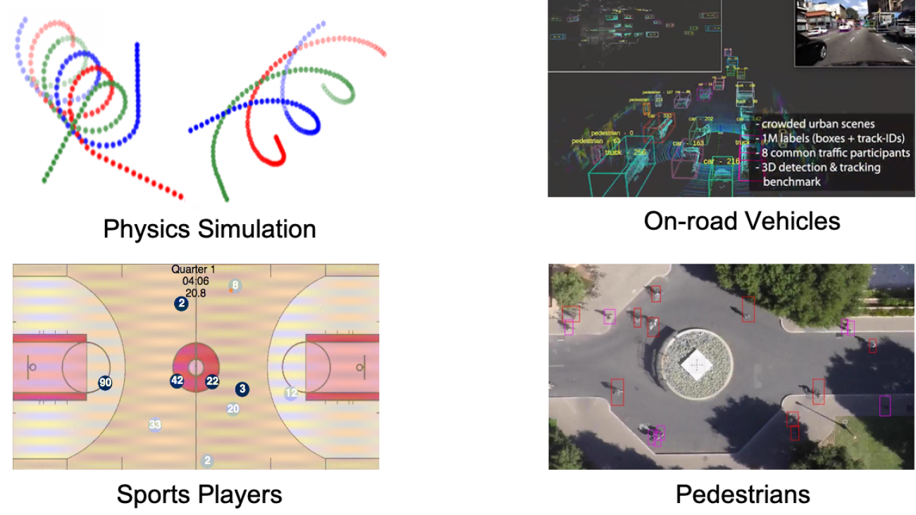
Multi-agent interacting systems are prevalent in the world, from purely physical systems to complicated social dynamic systems. The interactions between entities / components can give rise to very complex behavior patterns at the level of both individuals and the multi-agent system as a whole. Since usually only the trajectories of individual entities are observed without any knowledge of the underlying interaction patterns, and there are usually multiple possible modalities for each agent with uncertainty, it is challenging to model their dynamics and forecast their future behaviors.
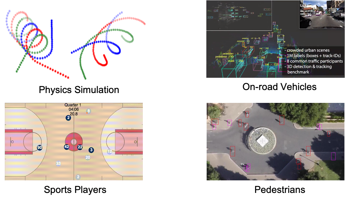
Figure 1. Typical multi-agent interacting systems.
In many real-world applications (e.g. autonomous vehicles, mobile robots), an effective understanding of the situation and accurate trajectory prediction of interactive agents play a significant role in downstream tasks, such as decision making and planning. We introduce a generic trajectory forecasting framework (named EvolveGraph) with explicit relational structure recognition and prediction via latent interaction graphs among multiple heterogeneous, interactive agents. Considering the uncertainty of future behaviors, the model is designed to provide multi-modal prediction hypotheses. Since the underlying interactions may evolve even with abrupt changes over time, and different modalities of evolution may lead to different outcomes, we address the necessity of dynamic relational reasoning and adaptively evolving the interaction graphs.