When translating the English phrase “How are you?” to Spanish, would you prefer to use “¿Cómo estás?” or “¿Cómo está usted?” instead?
Amazon Translate is a neural machine translation service that delivers fast, high-quality, and affordable language translation. Today, we’re excited to introduce Active Custom Translation (ACT), a feature that gives you more control over your machine translation output. You can now influence what machine translation output you would like to get between “¿Cómo estás?” or “¿Cómo está usted?”. To make ACT work, simply provide your translation examples in TMX, TSV, or CSV format to create parallel data (PD), and Amazon Translate uses your PD along with your batch translation job to customize the translation output at runtime. If you have PD that shows “How are you?” being translated to “¿Cómo está usted?”, ACT knows to customize the translation to “¿Cómo está usted?”.
Today, professional translators use examples of previous translations to provide more customized translations for customers. Similar to profession translators, Amazon Translate can now provide customized translations by learning from your translation examples.
Traditionally, this customization was done by creating a custom translation model—a specific-purpose translation engine built using customer data. Building custom translation models is complex, tedious, and expensive. It requires special expertise to prepare the data for training, testing, and validation. Then you build, deploy, and maintain the model by updating the model frequently. To save on model training and management costs, you may choose to delay updating your custom translation model, which means your models are always stale—negatively affecting your custom translation experience. In spite of all this work, these custom models perform well when the translation job is within the domain of your data. However, they tend to perform worse than a generic model when the translation job is outside of the domain of your customization data.
Amazon Translate ACT introduces an innovative way of providing customized translation output on the fly with your parallel data, without building a custom translation model. ACT output quality is always up to date with your PD. ACT provides the best translations for jobs both within the domain and outside the domain of PD. For example, if a source sentence isn’t in the domain of the PD, the translation output is still as good as the generic translation with no significant deterioration in translation quality. You no longer need to go through the tedious process of building and retraining custom translation models for each incoming use case. Just update the PD, and the ACT output automatically adapts to the most recent PD, without needing any retraining.
“Innovation is in our DNA. Our customers look to AWS to lead in customization of machine translation. Current custom translation technology is inefficient, cumbersome, and expensive,” says Marcello Federico, Principal Applied Scientist at Amazon Machine Learning, AWS. “Active Custom Translation allows our customers to focus on the value of their latest data and forget about the lifecycle management of custom translation models. We innovated on behalf of the customer to make custom machine translation easy.”
Don’t just take our word for it
Custom.MT implements machine translation for localization groups and translation companies. Konstantin Dranch, Custom.MT co-founder, shares, “Amazon Translate’s ACT is a breakthrough machine translation setup. A manual engine retraining takes 15–16 work hours, that’s why most language teams in the industry update their engines only once a month or once a quarter. With ACT, retraining is continuous and engines improve every day based on edits by human translators. Even before the feature was released to the market, we saw tremendous interest from leading software localization teams. With a higher quality of machine translation, enterprise teams can save millions of USD in manual translations and improve other KPIs, such as international user engagement and time to market.”
Welocalize is a leading global localization and translation company. Senior Manager of AI Deployments at Welocalize Alex Yanishevsky says, “Welocalize produces high-quality translations, so our customers can transform their content and data to grow globally and expand into international markets. Active Custom Translation from Amazon Translate allows us to customize our translations at runtime and provides us with significant flexibility in our production cycles. In addition, we see great business value and engine quality improvement since we can retrain engines frequently without incurring additional hosting or training charges.”
One Hour Translation is a leading professional language services provider. Yair Tal, CEO of One Hour Translation, says, “The customer demand for customized Neural Machine Translation (NMT) is growing every month because of the cost savings. As one of the first to try Amazon Translate ACT, we have found that ACT provides the best translation output for many language pairs. With ACT, training and maintenance is simple and the Translate API integrates with our system seamlessly. Translate’s pay-as-you-translate pricing helps our clients, both big and small, get translation output that is tailored for their needs without paying to train custom models.”
Building an Active Custom Translation job
Active Custom Translation’s capabilities are built right into the Amazon Translate experience. In this post, we walk you through the step-by-step process of using your data and getting a customized machine translated output securely. ACT is now available on batch translation, so first familiarize yourself with how to create a batch translation job.
You need data to customize your translation for terms or phrases that are unique to a specific domain, such as life sciences, law, or finance. You bring in examples of high-quality translations (source sentence and translated target sentence) in your preferred domain as a file in TMX, TSV, or CSV format. This data should also be UTF-8 encoded. You use this data to create a PD. Amazon Translate uses this PD to customize your machine translation. Each PD can be up to 1 GB large. You can upload up to 1,000 PD per account per Region. The 1,000 parallel data limit can be increased upon request. You get free storage for parallel data for up to 200 GB. You pay the local Amazon Simple Storage Service (Amazon S3) rate for excess data stored.
For our use case, I have my data in TSV format, and the name of my file is Mydata.tsv. I first upload this file to an S3 location (for this post, I store my data in s3://input-s3bucket/Paralleldata/).
The following table summarizes the contents of the file.
| en | es |
| Amazon Translate is a neural machine translation service. | Amazon Translate es un servicio de traducción automática basado en redes neuronales. |
| Neural machine translation is a form of language translation automation that uses deep learning models. | La traducción automática neuronal es una forma de automatizar la traducción de lenguajes utilizando modelos de aprendizaje profundo. |
| How are you? | ¿Cómo está usted? |
We run this example in the US West (Oregon) Region, us-west-2.
CreateParallelData
Calling the CreateParallelData API creates a PD resource record in our database and asynchronously starts a workflow for processing the PD file and ingesting it into our service.
CLI
The following CLI commands are formatted for Unix, Linux, and macOS. For Windows, replace the backslash () Unix continuation character at the end of each line with a caret (^).
Run the following CLI command:
aws translate create-parallel-data
--name ${PARALLEL_DATA_NAME}
--parallel-data-config S3Uri=${S3_URI},Format=${FORMAT}
--region ${REGION}
I use Mydata.tsv to create my PD my-parallel-data-1:
aws translate create-parallel-data
--name my-parallel-data-1
--parallel-data-config S3Uri= s3://input-s3bucket/Paralleldata/Mydata.tsv,Format=TSV
--region us-west-2
You get a response like the following code:
{
    "Name": "my-parallel-data-1",
    "Status": "CREATING"
}
This means that your PD is being created now.
Run aws translate create-parallel-data help for more information.
Console
To use the Amazon Translate console, complete the following steps:
- On the Amazon Translate console, under Customization, choose Parallel data.
- Choose Create parallel data.

- For Name, insert
my-parallel-data-1. - For Parallel data location in S3, enter your S3 location (for this post,
s3://input-s3bucket/Paralleldata/Mydata.tsv). - For File format¸ you can choose CSV, TSV, or TMX. For this post, we choose Tab-separated values (.tsv).
Your data is always secure with Amazon Translate. It’s encrypted using an AWS owned encryption key by default. You can encrypt it using a key from your current account or use a key from a different account.
- For this post, for Encryption key, we select Use AWS owned key.
- Choose Create parallel data.

ListParallelData
Calling the ListParallelData API returns a list of PD that exists and their details (it doesn’t include a pre-signed Amazon S3 URL for downloading the data)
CLI
Run the following CLI command:
aws translate list-parallel-data
--region us-west-2
You get a response like the following code:
{
    "ParallelDataPropertiesList": [
        {
            "Name": "my-parallel-data-1",
            "Arn": "arn:aws:translate:us-west-2:123456789012:parallel-data/my-parallel-data-1",
            "Status": "ACTIVE",
            "SourceLanguageCode": "en",
            "TargetLanguageCodes": [
                "es"
            ],
            "ParallelDataConfig": {
                "S3Uri": "s3://input-s3bucket/Paralleldata/Mydata.tsv",
                "Format": "TSV"
            },
            "ImportedDataSize": 532,
            "ImportedRecordCount": 3,
            "FailedRecordCount": 0,
            "CreatedAt": 1234567890.406,
            "LastUpdatedAt": 1234567890.675
        }
    ]
}
The "Status": "ACTIVE" means your PD is ready for you to use.
Run aws translate list-parallel-data help for more information.
Console
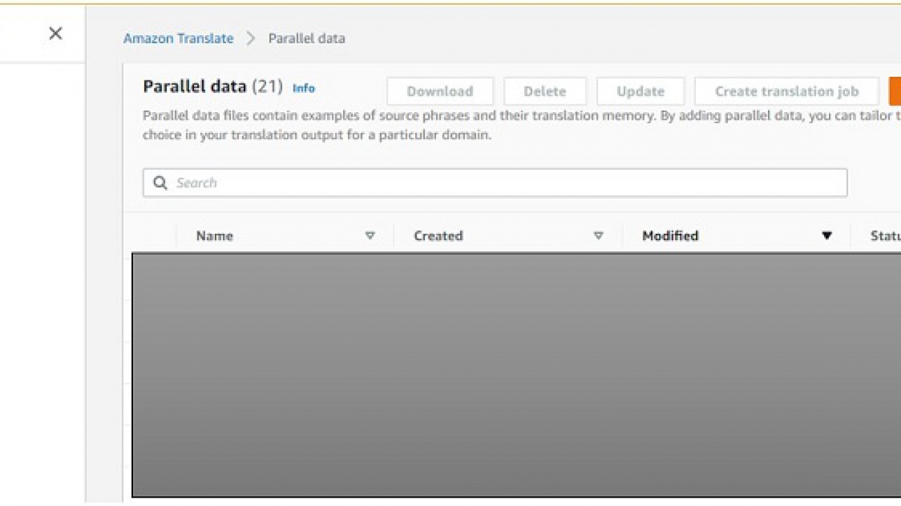
This following screenshot shows the result for list-parallel-data on the Amazon Translate console.

GetParallelData
Calling the GetParallelData API returns details of the named parallel data and a pre-signed Amazon S3 URL for downloading the data.
CLI
Run the following CLI command:
aws translate get-parallel-data
--name ${PARALLEL_DATA_NAME}
--region ${REGION}
For example, my code looks like the following:
aws translate get-parallel-data
--name my-parallel-data-1
--region us-west-2
You get a response like the following code:
{
    "ParallelDataProperties": {
        "Name": "my-parallel-data-1",
        "Arn": "arn:aws:translate:us-west-2:123456789012:parallel-data/my-parallel-data-1",
        "Status": "ACTIVE",
        "SourceLanguageCode": "en",
        "TargetLanguageCodes": [
            "es"
        ],
        "ParallelDataConfig": {
            "S3Uri": "s3://input-s3bucket/Paralleldata/Mydata.tsv",
            "Format": "TSV"
        },
        "ImportedDataSize": 532,
        "ImportedRecordCount": 3,
        "FailedRecordCount": 0,
        "CreatedAt": 1234567890.406,
        "LastUpdatedAt": 1234567890.675
    },
    "DataLocation": {
        "RepositoryType": "S3",
        "Location": "xxx"
    }
}
“Location” contains the pre-signed Amazon S3 URL for downloading the data.
Run aws translate get-parallel-data help for more information.
Console
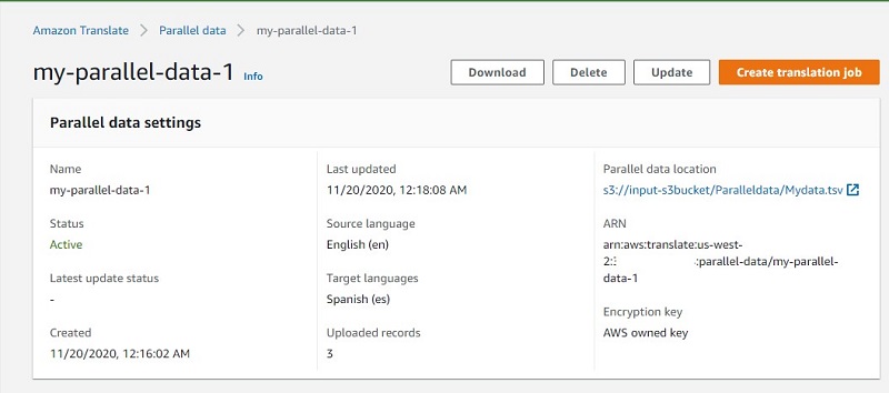
On the Amazon Translate console, choose one of the PD files on the Parallel data page.

You’re directed to another page that includes the detail for this parallel data file. The following screenshot shows the details for get-parallel-data.

UpdateParallelData
Calling the UpdateParallelData API replaces the old parallel data with the new one.
CLI
Run the following CLI command:
aws translate update-parallel-data
--name ${PARALLEL_DATA_NAME}
--parallel-data-config S3Uri=${NEW_S3_URI},Format=${FORMAT}
--region us-west-2
For this post, Mydata1.tsv is my new parallel data. My code looks like the following:
aws translate update-parallel-data
--name my-parallel-data-1
--parallel-data-config S3Uri= s3://input-s3bucket/Paralleldata/Mydata1.tsv,Format=TSV
--region us-west-2
You get a response like the following code:
{
    "Name": "my-parallel-data-1",
    "Status": "ACTIVE",
    "LatestUpdateAttemptStatus": "UPDATING",
    "LatestUpdateAttemptAt": 1234567890.844
}
The "LatestUpdateAttemptStatus": "UPDATING" means your parallel data is being updated now.
Wait for a few minutes and run get-parallel-data again. You can see the parallel data get updated, such as in the following code:
{
    "ParallelDataProperties": {
            "Name": "my-parallel-data-1",
            "Arn": "arn:aws:translate:us-west-2:123456789012:parallel-data/my-parallel-data-1",
            "Status": "ACTIVE",
            "SourceLanguageCode": "en",
            "TargetLanguageCodes": [
                "es"
            ],
            "ParallelDataConfig": {
                "S3Uri": "s3://input-s3bucket/Paralleldata/Mydata1.tsv",
                "Format": "TSV"
            },
        ...
    }
}
We can see that the parallel data has been updated from Mydata.tsv to Mydata1.tsv.
Run aws translate update-parallel-data help for more information.
Console
On the Amazon Translate console, choose the parallel data file and choose Update.
You can replace the new parallel data file with the existing one by specifying the new Amazon S3 URL.
Creating your first Active Custom Translation job
In this section, we discuss the different ways you can create your ACT job.
StartTextTranslationJob
Calling the StartTextTranslationJob starts a batch translation. When you add parallel data to a batch translation job, you create an ACT job. Amazon Translate customizes your ACT output to match the style, tone, and word choices it finds in your PD. ACT is a premium product, so see Amazon Translate pricing for pricing information. You can only specify one parallel data file to use with the text translation job.
CLI
Run the following command:
aws translate start-text-translation-job
--input-data-config ContentType=${CONTENT_TYPE},S3Uri=${INPUT_S3_URI}
--output-data-config S3Uri=${OUTPUT_S3_URI}
--data-access-role-arn ${DATA_ACCESS_ROLE}
--source-language-code=${SOURCE_LANGUAGE_CODE} --target-language-codes=${TARGET_LANGUAGE_CODE}
--parallel-data-names ${PARALLEL_DATA_NAME}
--region ${REGION}
--job-name ${JOB_NAME}
For example, my code looks like the following:
aws translate start-text-translation-job
--input-data-config ContentType=application/vnd.openxmlformats-officedocument.spreadsheetml.sheet,S3Uri= s3://input-s3bucket/inputfile/
--output-data-config S3Uri= s3://output-s3bucket/Output/
--data-access-role-arn arn:aws:iam::123456789012:role/TranslateBatchAPI
--source-language-code=en --target-language-codes=es
--parallel-data-names my-parallel-data-1
--region us-west-2
--job-name ACT1
You get a response like the following code:
{
    "JobId": "4446f95f20c88a4b347449d3671fbe3d",
    "JobStatus": "SUBMITTED"
}
This output means the job has been submitted successfully.
Run aws translate start-text-translation-job help for more information.
Console
For instructions on running a batch translation job on the Amazon Translate console, see Translating documents, spreadsheets, and presentations in Office Open XML format using Amazon Translate. Choose my-parallel-data-1 as the parallel data to create your first ACT job, ACT1.

Congratulations! You have created your first ACT job. ACT is available in the following Regions:
- US East (Northern Virginia)
- US West (Oregon)
- Europe (Ireland)
Running your Active Custom Translation job
ACT works on asynchronous batch translation for language pairs that have English as either the source or target language.
Now, let’s try to translate the following text from English to Spanish and see how ACT helps to customize the output:
“How are you?” is one of the most common questions you’ll get asked when meeting someone. The most common response is “good”
The following is the output you get when you translate without any customization:
“¿Cómo estás?” es una de las preguntas más comunes que se le harán cuando conozca a alguien. La respuesta más común es “Buena”
The following is the output you get when you translate using ACT with my-parallel-data-1 as the PD:
“¿Cómo está usted?” es una de las preguntas más comunes que te harán cuando te reúnas con alguien. La respuesta más común es “Buena”
Conclusion
Amazon Translate ACT introduces a powerful way of providing personalized translation output with the following benefits:
- You don’t have to build a custom translation model
- You only pay for what you translate using ACT
- There is no additional model building or model hosting cost
- Your data is always secure and always under your control
- You get the best machine translation even when your source text is outside the domain of your parallel data
- You can update your parallel data as often as you need for no additional cost
Try ACT today. Bring your parallel data and start customizing your machine translation output. For more information about Amazon Translate ACT, see Asynchronous Batch Processing.
Related resources
For additional resources, see the following:
- Amazon Translate FAQs
- Translate Text Between Languages in the Cloud
- Translating documents, spreadsheets, and presentations in Office Open XML format using Amazon Translate
- Amazon Translate Developer Guide
About the Authors
 Watson G. Srivathsan is the Sr. Product Manager for Amazon Translate, AWS’s natural language processing service. On weekends you will find him exploring the outdoors in the Pacific Northwest.
 Xingyao Wang is the Software Develop Engineer for Amazon Translate, AWS’s natural language processing service. She likes to hang out with her cats at home.


 David Shute is a Senior ML GTM Specialist at Amazon Web Services focused on Amazon Kendra. When not working, he enjoys hiking and walking on a beach.
 Juan Pablo Bustos is an AI Services Specialist Solutions Architect at Amazon Web Services, based in Dallas, TX. Outside of work, he loves spending time writing and playing music as well as trying random restaurants with his family.
 Anuj Gupta is the Product Manager for Amazon Augmented AI. He is focusing on delivering products that make it easier for customers to adopt machine learning. In his spare time, he enjoys road trips and watching Formula 1.


 Frank Wang is a Startup Senior Solutions Architect at AWS. He has worked with a wide range of customers with focus on Independent Software Vendors (ISVs) and now startups. He has several years of engineering leadership, software architecture, and IT enterprise architecture experiences, and now focuses on helping customers through their cloud journey on AWS.
 Shishuai Wang is an ML Specialist Solutions Architect working with the AWS WWSO team. He works with AWS customers to help them adopt machine learning on a large scale. He enjoys watching movies and traveling around the world.
 Yu Zhang is a staff software engineer and the technical lead of the Deep Learning platform at DeepMap. His research interests include Large-Scale Image Concept Learning, Image Retrieval, and Geo and Climate Informatic
 Tom Wang is a founding team member and Director of Engineering at DeepMap, managing their cloud infrastructure, backend services, and map pipelines. Tom has 20+ years of industry experience in database storage systems, distributed big data processing, and map data infrastructure. Prior to DeepMap, Tom was a tech lead at Apple Maps and key contributor to Apple’s map data infrastructure and map data validation platform. Tom holds an MS degree in computer science from the University of Wisconsin-Madison.