Can AI make me trendier?

Can AI make me trendier?

As a software engineer and generally analytic type, I like to craft theories for everything. Theories on how to build software, how to stay productive, how to be creative…and even how to dress well. For help with that last one, I decided to hire a personal stylist. As it turned out, I was not my stylist’s first software engineer client. “The problem with you people in tech is that you’re always looking for some sort of theory of fashion,” she told me. “But there is no formula–it’s about taste.”

Unfortunately my stylist’s taste was a bit outside of my price range (I drew the line at a $300 hoodie). But I knew she was right. It’s true that computers (and maybe the people who program them) are better at solving problems with clear-cut answers than they are at navigating touchy-feely matters, like taste. Fashion trends are not set by data-crunching CPUs, they’re made by human tastemakers and fashionistas and their modern-day equivalents, social media influencers. 

I found myself wondering if I could build an app that combined trendsetters’ sense of style with AI’s efficiency to help me out a little. I started getting fashion inspiration from Instagram influencers who matched my style. When I saw an outfit I liked, I’d try to recreate it using items I already owned. It was an effective strategy, so I set out to automate it with AI.

First, I partnered up with one of my favorite programmers, who just so happened to also be an Instagram influencer, Laura Medalia (or codergirl_ on Instagram). With her permission, I uploaded all of Laura’s pictures to Google Cloud to serve as my outfit inspiration.

Image showing a screenshot of the Instagram profile of "codergirl."

Next, I painstakingly photographed every single item of clothing I owned, creating a digital archive of my closet.

Animated GIF showing a woman in a white room placing different clothing items on a mannequin and taking photos of them.

To compare my closet with Laura’s, I used Google Cloud Vision Product Search API, which uses computer vision to identify similar products. If you’ve ever seen a “See Similar Items” tab when you’re online shopping, it’s probably powered by a similar technology. I used this API to look through all of Laura’s outfits and all of my clothes to figure out which looks I could recreate. I bundled up all of the recommendations into a web app so that I could browse them on my phone, and voila: I had my own AI-powered stylist. It looks like this:

Animated GIF showing different screens that display items of clothing that can be paired together to create an outfit.

Thanks to Laura’s sense of taste, I have lots of new ideas for styling my own wardrobe. Here’s one look I was able to recreate:

Image showing two screens; on the left, a woman is standing in a room wearing a fashionable outfit with the items that make up that outfit in two panels below her. In the other is another woman, wearing a similar outfit.

If you want to see the rest of my newfound outfits, check out the YouTube video at the top of this post, where I go into all of the details of how I built the app, or read my blog post.

No, I didn’t end up with a Grand Unified Theory of Fashion—but at least I have something stylish to wear while I’m figuring it out.

Read More

Transformers for Image Recognition at Scale

Transformers for Image Recognition at Scale

Posted by Neil Houlsby and Dirk Weissenborn, Research Scientists, Google Research

While convolutional neural networks (CNNs) have been used in computer vision since the 1980s, they were not at the forefront until 2012 when AlexNet surpassed the performance of contemporary state-of-the-art image recognition methods by a large margin. Two factors helped enable this breakthrough: (i) the availability of training sets like ImageNet, and (ii) the use of commoditized GPU hardware, which provided significantly more compute for training. As such, since 2012, CNNs have become the go-to model for vision tasks.

The benefit of using CNNs was that they avoided the need for hand-designed visual features, instead learning to perform tasks directly from data “end to end”. However, while CNNs avoid hand-crafted feature-extraction, the architecture itself is designed specifically for images and can be computationally demanding. Looking forward to the next generation of scalable vision models, one might ask whether this domain-specific design is necessary, or if one could successfully leverage more domain agnostic and computationally efficient architectures to achieve state-of-the-art results.

As a first step in this direction, we present the Vision Transformer (ViT), a vision model based as closely as possible on the Transformer architecture originally designed for text-based tasks. ViT represents an input image as a sequence of image patches, similar to the sequence of word embeddings used when applying Transformers to text, and directly predicts class labels for the image. ViT demonstrates excellent performance when trained on sufficient data, outperforming a comparable state-of-the-art CNN with four times fewer computational resources. To foster additional research in this area, we have open-sourced both the code and models.

The Vision Transformer treats an input image as a sequence of patches, akin to a series of word embeddings generated by a natural language processing (NLP) Transformer.

The Vision Transformer
The original text Transformer takes as input a sequence of words, which it then uses for classification, translation, or other NLP tasks. For ViT, we make the fewest possible modifications to the Transformer design to make it operate directly on images instead of words, and observe how much about image structure the model can learn on its own.

ViT divides an image into a grid of square patches. Each patch is flattened into a single vector by concatenating the channels of all pixels in a patch and then linearly projecting it to the desired input dimension. Because Transformers are agnostic to the structure of the input elements we add learnable position embeddings to each patch, which allow the model to learn about the structure of the images. A priori, ViT does not know about the relative location of patches in the image, or even that the image has a 2D structure — it must learn such relevant information from the training data and encode structural information in the position embeddings.

Scaling Up

We first train ViT on ImageNet, where it achieves a best score of 77.9% top-1 accuracy. While this is decent for a first attempt, it falls far short of the state of the art — the current best CNN trained on ImageNet with no extra data reaches 85.8%. Despite mitigation strategies (e.g., regularization), ViT overfits the ImageNet task due to its lack of inbuilt knowledge about images.

To investigate the impact of dataset size on model performance, we train ViT on ImageNet-21k (14M images, 21k classes) and JFT (300M images, 18k classes), and compare the results to a state-of-the-art CNN, Big Transfer (BiT), trained on the same datasets. As previously observed, ViT performs significantly worse than the CNN equivalent (BiT) when trained on ImageNet (1M images). However, on ImageNet-21k (14M images) performance is comparable, and on JFT (300M images), ViT now outperforms BiT.

Finally, we investigate the impact of the amount of computation involved in training the models. For this, we train several different ViT models and CNNs on JFT. These models span a range of model sizes and training durations. As a result, they require varying amounts of compute for training. We observe that, for a given amount of compute, ViT yields better performance than the equivalent CNNs.

Left: Performance of ViT when pre-trained on different datasets. Right: ViT yields a good performance/compute trade-off.

High-Performing Large-Scale Image Recognition
Our data suggest that (1) with sufficient training ViT can perform very well, and (2) ViT yields an excellent performance/compute trade-off at both smaller and larger compute scales. Therefore, to see if performance improvements carried over to even larger scales, we trained a 600M-parameter ViT model.

This large ViT model attains state-of-the-art performance on multiple popular benchmarks, including 88.55% top-1 accuracy on ImageNet and 99.50% on CIFAR-10. ViT also performs well on the cleaned-up version of the ImageNet evaluations set “ImageNet-Real”, attaining 90.72% top-1 accuracy. Finally, ViT works well on diverse tasks, even with few training data points. For example, on the VTAB-1k suite (19 tasks with 1,000 data points each), ViT attains 77.63%, significantly ahead of the single-model state of the art (SOTA) (76.3%), and even matching SOTA attained by an ensemble of multiple models (77.6%). Most importantly, these results are obtained using fewer compute resources compared to previous SOTA CNNs, e.g., 4x fewer than the pre-trained BiT models.

Vision Transformer matches or outperforms state-of-the-art CNNs on popular benchmarks. Left: Popular image classification tasks (ImageNet, including new validation labels ReaL, and CIFAR, Pets, and Flowers). Right: Average across 19 tasks in the VTAB classification suite.

Visualizations
To gain some intuition into what the model learns, we visualize some of its internal workings. First, we look at the position embeddings — parameters that the model learns to encode the relative location of patches — and find that ViT is able to reproduce an intuitive image structure. Each position embedding is most similar to others in the same row and column, indicating that the model has recovered the grid structure of the original images. Second, we examine the average spatial distance between one element attending to another for each transformer block. At higher layers (depths of 10-20) only global features are used (i.e., large attention distances), but the lower layers (depths 0-5) capture both global and local features, as indicated by a large range in the mean attention distance. By contrast, only local features are present in the lower layers of a CNN. These experiments indicate that ViT can learn features hard-coded into CNNs (such as awareness of grid structure), but is also free to learn more generic patterns, such as a mix of local and global features at lower layers, that can aid generalization.

Left: ViT learns the grid like structure of the image patches via its position embeddings. Right: The lower layers of ViT contain both global and local features, the higher layers contain only global features.

Summary
While CNNs have revolutionized computer vision, our results indicate that models tailor-made for imaging tasks may be unnecessary, or even sub-optimal. With ever-increasing dataset sizes, and the continued development of unsupervised and semi-supervised methods, the development of new vision architectures that train more efficiently on these datasets becomes increasingly important. We believe ViT is a preliminary step towards generic, scalable architectures that can solve many vision tasks, or even tasks from many domains, and are excited for future developments.

A preprint of our work as well as code and models are publically available.

Acknowledgements
We would like to thank our co-authors in Berlin, Zürich, and Amsterdam: Alexey Dosovitskiy, Lucas Beyer, Alexander Kolesnikov, Xiaohua Zhai, Thomas Unterthiner, Mostafa Dehghani, Matthias Minderer, Georg Heigold, Sylvain Gelly, and Jakob Uszkoreit. We would like to thank Andreas Steiner for crucial help with infrastructure and open-sourcing, Joan Puigcerver and Maxim Neumann for work on large-scale training infrastructure, and Dmitry Lepikhin, Aravindh Mahendran, Daniel Keysers, Mario Lučić, Noam Shazeer, and Colin Raffel for useful discussions. Finally, we thank Tom Small for creating the Visual Transformer animation in this post.

Read More

Big Wheels Keep on Learnin’: Einride’s AI Trucks Advance Capabilities with NVIDIA DRIVE AGX Orin

Big Wheels Keep on Learnin’: Einride’s AI Trucks Advance Capabilities with NVIDIA DRIVE AGX Orin

Swedish startup Einride has rejigged the big rig for highways around the world.

The autonomous truck maker launched the next generation of its cab-less autonomous truck, known as the Pod, with new, advanced functionality and pricing. The AI vehicles, which will be commercially available worldwide, will be powered by the latest in high-performance, energy-efficient compute — NVIDIA DRIVE AGX Orin.

These scalable self-driving haulers will begin to hit the road in 2023, with a variety of models available to customers around the world.

Autonomous trucks are always learning, taking in vast amounts of data to navigate the unpredictability of the real world, from highways to crowded ports. This rapid processing requires centralized, high-performance AI compute.

With the power of AI, these vehicles can easily rise to the demands of the trucking industry. The vehicles can operate 24 hours a day, improving delivery times. And, with increased efficiency, they can slash the annual cost of logistics in the U.S. by 45 percent, according to experts at McKinsey.

Einride’s autonomous pods and trucks are built for every type of route. They can automate short, routine trips like the loading and unloading of containers on cargo ships and managing port operations, as well as autonomously drive on the highway, dramatically streamlining the shipping and logistics.

A New Pod Joins the Squad

The latest Einride Pod features a refined design that balances sleek features with the practical requirements of wide-scale production.

Its rounded edges give it an aerodynamic shape for greater efficiency and performance, without sacrificing cargo space. The Pod’s lighting system — which includes headlights, tail lights and indicators — provides a signature look while improving visibility for road users.

The cab-less truck comes in a range of variations, depending on use case. The AET 1 (Autonomous Electric Transport) model is purpose-built for closed facilities with dedicated routes — such as a port or loading bay. The AET 2 can handle fenced-in areas as well as short-distance public roads between destinations.

The AET 3 and AET 4 vehicles are designed for fully autonomous operation on backroads and highways, with speeds of up to 45 km per hour.

Einride is currently accepting reservations for AET 1 and AET 2, with others set to ship starting in 2022.

Trucking Ahead with Orin

The Einride Pod is able to achieve its scalability and autonomous functionality by leveraging the next generation in AI compute.

NVIDIA Orin is a system-on-a-chip born out of the data center, consisting of 17 billion transistors and the result of four years of R&D investment. It achieves 200 TOPS — nearly 7x the performance of the previous generation SoC Xavier — and is designed to handle the large number of applications and deep neural networks that run simultaneously in autonomous trucks, while achieving systematic safety standards such as ISO 26262 ASIL-D.

This massive compute capability ensures the Einride Pod is continuously learning, expanding the environments and situations in which it can operate autonomously.

These next-generation electric, self-driving freight transport vehicles built on NVIDIA DRIVE are primed to safely increase productivity, improve utilization, reduce emissions and decrease the world’s dependence on fossil fuels.

The post Big Wheels Keep on Learnin’: Einride’s AI Trucks Advance Capabilities with NVIDIA DRIVE AGX Orin appeared first on The Official NVIDIA Blog.

Read More

Chalk and Awe: Studio Crafts Creative Battle Between Stick Figures with Real-Time Rendering

Chalk and Awe: Studio Crafts Creative Battle Between Stick Figures with Real-Time Rendering

It’s time to bring krisp graphics to stick figure drawings.

Creative studio SoKrispyMedia, started by content creators Sam Wickert and Eric Leigh, develops short videos blended with high-quality visual effects. Since publishing one of their early works eight years ago on YouTube, Chalk Warfare 1, the team has regularly put out short films that showcase engaging visual effects and graphics — including Stick Figure Battle, which has nearly 25 million views.

Now, the Stick Figure saga continues with SoKrispyMedia’s latest, Stick Figure War, which relies on real-time rendering for photorealistic results, as well as improved creative workflows.

With real-time rendering, SoKrispyMedia worked more efficiently as they could see the final results quickly, and have more time for iterations so they could ensure the visuals looked exactly how they wanted — from stick figures piloting paper airplanes to robots fighting skeletons in textbooks.

The team enhanced their virtual production process by using Unreal Engine and a Dell Precision 7750 mobile workstation featuring an NVIDIA Quadro RTX 5000 GPU. Adding to this mix high-quality cameras and DaVinci Resolve software from Blackmagic Design, SoKrispyMedia produced a short film with higher quality than they ever thought possible.

Real-Time Rendering Sticks Out in Visual Effects

Integrating real-time rendering into their pipelines has allowed SoKrispyMedia to work faster and iterate more quickly. They no longer need to wait hundreds of hours for renders to preview — everything can be produced in real time.

“Looking back at our older videos and the technology we used, it feels like we were writing in pencil, and as the technology evolves, we’re adding more and more colors to our palette,” said Micah Malinics, producer at SoKrispyMedia.

For Stick Figure War, a lot of the elements in the video were drawn by hand, and then scanned and converted into 2D or 3D graphics in Unreal Engine. The creators also developed a stylized filter that allowed them to make certain elements look like cross-hatched drawings.

SoKrispyMedia used Unreal Engine to do real-time rendering for almost the entire film, which enabled them to explore more creative ideas and let their imaginations run wild without worrying about increased render times.

Pushing Creativity Behind the Scenes

While NVIDIA RTX and Unreal Engine have broadened the reach of real-time rendering, Blackmagic Design has made high-quality cameras more accessible so content creators can produce cinematic-quality work at a fraction of the cost.

For Stick Figure War, SoKrispyMedia used Blackmagic URSA Mini G2 for production, Pocket Cinema Camera for pick-up shots and Micro Studio Camera 4K for over-the-head VFX shots. With the cameras, the team could shoot videos at 4K resolution and crop footage without losing any resolution in post-production.

Editing workflows were accelerated as Blackmagic’s DaVinci Resolve utilized NVIDIA GPUs to dramatically speed up playback and performance.

“Five to 10 years ago, making this video would’ve been astronomically difficult. Now we’re able to simply plug the Blackmagic camera directly into Unreal and see final results in front of our eyes,” said Sam Wickert, co-founder of SoKrispyMedia. “Using the Resolve Live feature for interactive and collaborative color grading and editing is just so fast, easy and efficient. We’re able to bring so much more to life on screen than we ever thought possible.”

The SoKrispyMedia team was provided with a Dell Precision 7750 mobile workstation with an RTX 5000 GPU inside, allowing the content creators to work on the go and preview real-time renderings on set. And the Dell workstation’s display provided advanced color accuracy, from working in DaVinci Resolve to rendering previews and final images.

Learn more about the making of SoKrispyMedia’s latest video, Stick Figure War.

The post Chalk and Awe: Studio Crafts Creative Battle Between Stick Figures with Real-Time Rendering appeared first on The Official NVIDIA Blog.

Read More

Performing simulations at scale with Amazon SageMaker Processing and R on RStudio

Performing simulations at scale with Amazon SageMaker Processing and R on RStudio

Statistical analysis and simulation are prevalent techniques employed in various fields, such as healthcare, life science, and financial services. The open-source statistical language R and its rich ecosystem with more than 16,000 packages has been a top choice for statisticians, quant analysts, data scientists, and machine learning (ML) engineers. RStudio is an integrated development environment (IDE) designed for data science and statistics for R users. However, an RStudio IDE hosted on a single machine used for day-to-day interactive statistical analysis isn’t suited for large-scale simulations that can require scores of GB of RAM (or more). This is especially difficult for scientists wanting to run analyses locally on a laptop or a team of statisticians developing in RStudio on one single instance.

In this post, we show you a solution that allows you to offload a resource-intensive Monte Carlo simulation to more powerful machines, while still being able to develop your scripts in your RStudio IDE. This solution takes advantage of Amazon SageMaker Processing.

Amazon SageMaker and SageMaker Processing

Amazon SageMaker is a fully managed service that provides every developer and data scientist with the ability to build, train, and deploy ML models quickly. SageMaker removes the heavy lifting from each step of the ML process to make it easier to develop high-quality ML artifacts. Running workloads on SageMaker is easy. When you’re ready to fit a model in SageMaker, simply specify the location of your data in Amazon Simple Storage Service (Amazon S3) and indicate the type and quantity of SageMaker ML instances you need. SageMaker sets up a distributed compute cluster, performs the training, outputs the result to Amazon S3, and tears down the cluster when complete.

SageMaker Processing allows you to quickly and easily perform preprocessing and postprocessing on data using your own scripts or ML models. This use case fits the pattern of many R and RStudio users, who frequently perform custom statistical analysis using their own code. SageMaker Processing uses the AWS Cloud infrastructure to decouple the development of the R script from its deployment, and gives you flexibility to choose the instance it’s deployed on. You’re no longer limited to the RAM and disk space limitations of the machine you develop on; you can deploy the simulation on a larger instance of your choice.

Another major advantage of using SageMaker Processing is that you’re only billed (per second) for the time and resources you use. When your script is done running, the resources are shut down and you’re no longer billed beyond that time.

Statisticians and data scientists using the R language can access SageMaker features and the capability to scale their workload via the Reticulate library, which provides an R interface to the SageMaker Python SDK library. Reticulate embeds a Python session within your R session, enabling seamless, high-performance interoperability. The Reticulate package provides an R interface to make API calls to SageMaker with the SageMaker Python SDK. We use Reticulate to interface SageMaker Python SDK in this post.

Alternatively, you can access SageMaker and other AWS services via Paws. Paws isn’t an official AWS SDK, but it covers most of the same functionality as the official SDKs for other languages. For more information about accessing AWS resources using Paws, see Getting started with R on Amazon Web Services.

In this post, we demonstrate how to run non-distributed, native R programs with SageMaker Processing. If you have distributed computing use cases using Spark and SparkR within RStudio, you can use Amazon EMR to power up your RStudio instance. To learn more, see the following posts:

Use case

In many use cases, more powerful compute instances are desired for developers conducting analyses on RStudio. For this post, we consider the following use case: the statisticians in your team have developed a Monte Carlo simulation in the RStudio IDE. The program requires some R libraries and it runs smoothly with a small number of iterations and computations. The statisticians are cautious about running a full simulation because RStudio is running on an Amazon Elastic Compute Cloud (Amazon EC2) instance shared by 10 other statisticians on the same team. You’re all running R analyses at a certain scale, which that makes the instance very busy most of the time. If anyone starts a full-scale simulation, it slows everyone’s RStudio session and possibly freezes the RStudio instance.

Even for a single user, running a large-scale simulation on a small- or a mid-sized EC2 instance is a problem that this solution can solve.

To walk through the solution for this use case, we designed a Monte Carlo simulation: given an area of certain width and length and a certain number of people, the simulation randomly places the people in the area and calculates the number of social distancing violations; each time a person is within 6 units of another, two violations are counted (because each person is violating the social distance rules). The simulation then calculates the average violation per person. For example, if there are 10 people and two violations, the average is 0.2. How many violations occur is also a function of how the people in the area are positioned. People can be bunched together, causing many violations, or spread out, causing fewer violations. The simulation performs many iterations of this experiment, randomly placing people in the area for each iteration (this is the characteristic that makes it a Monte Carlo simulation).

Solution overview

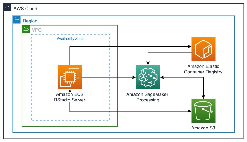
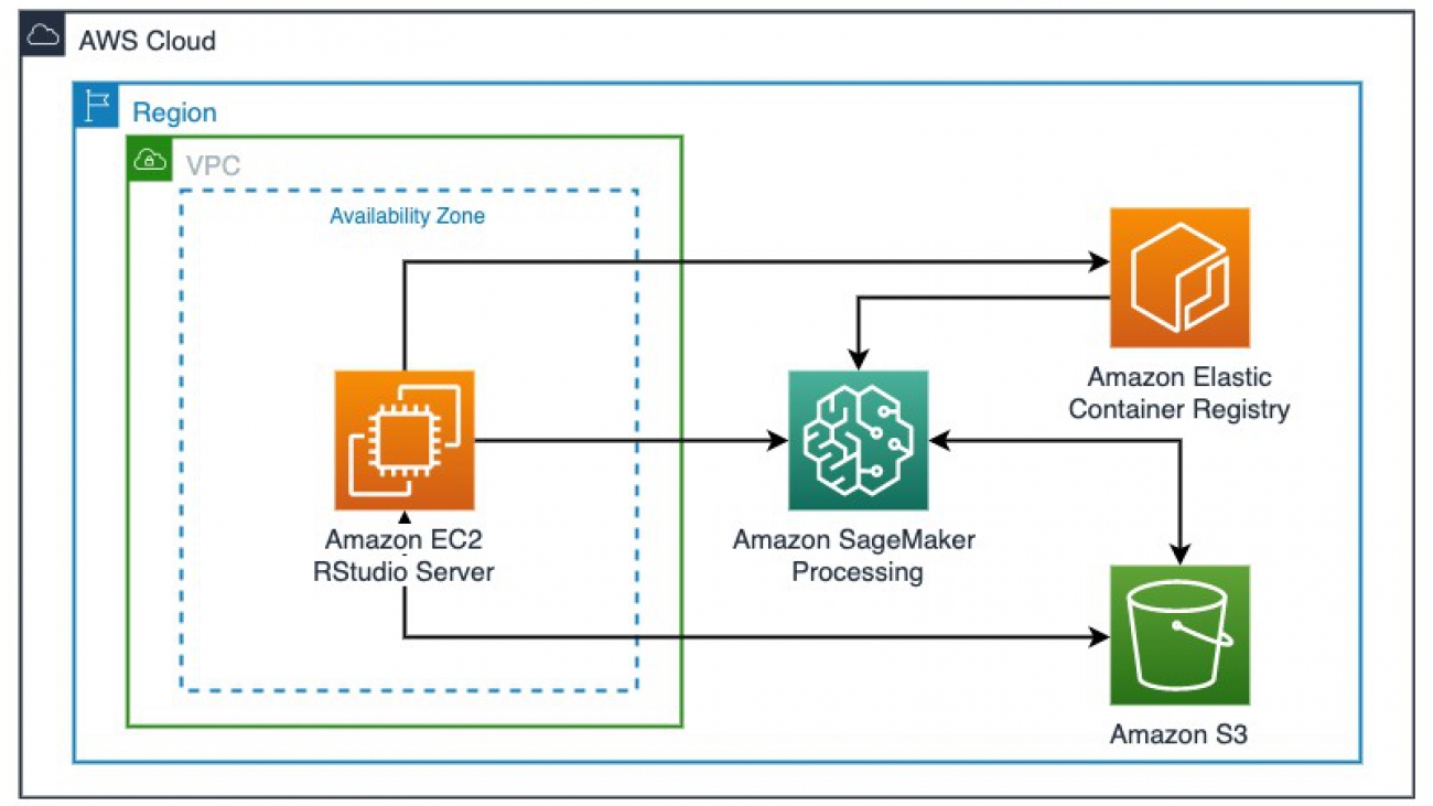
With a couple of lines of R code and a Docker container that encapsulates the runtime dependencies, you can dispatch the simulation program to the fully managed SageMaker compute infrastructure with the desired compute resources at scale. You can interactively submit the simulation script from within RStudio hosted on an EC2 instance to SageMaker Processing with a user-defined Docker container hosted on Amazon Elastic Container Registry (Amazon ECR) and data located on Amazon S3 (we discuss Docker container basics in the Building an R container in RStudio IDE and hosting it in Amazon ECR section). SageMaker Processing takes care of provisioning the infrastructure, running the simulation, reading and saving the data to Amazon S3, and tearing tear down the compute without any manual attention on the infrastructure.

The following diagram illustrates this solution architecture.

Deploying the resources

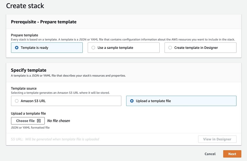
We first deploy an RStudio Server on an EC2 instance inside a VPC using an AWS CloudFormation template, which is largely based on the post Using R with Amazon SageMaker with some modifications. In addition to the RStudio Server, we install the Docker engine, SageMaker Python SDK, and Reticulate as part of the deployment. To deploy your resources, complete the following steps:

  1. Download the CloudFormation template
  2. On the AWS CloudFormation console, choose Template is ready.
  3. Choose Upload a template file.
  4. Choose Choose file.
  5. Upload the provided ec2_ubuntu_rstudio_sagemaker.yaml template.

The template is designed to work in the following Regions:

  • us-east-1
  • us-east-2
  • us-west-2
  • eu-west-1

In the YAML file, you can change the instance type to a different instance. For this workload, we recommend an instance no smaller than a t3.xlarge for running RStudio smoothly.

  1. Choose Next.

  1. For Stack name, enter a name for your stack.
  2. For AcceptRStudioLicenseAndInstall, review and accept the AGPL v3 license for installing RStudio Server on Amazon EC2.
  3. For KeyName, enter an Amazon EC2 key pair that you have previously generated to access an Amazon EC2 instance.

For instructions on creating a key pair, see Amazon EC2 key pairs and Linux instances.

  1. Choose Next.
  2. In the Configure stack options section, keep everything at their default values.
  3. Choose Next.
  4. Review the stack details and choose Create stack.

Stack creation takes about 15-20 minutes to complete.

  1. When stack creation is complete, go to the stack’s Outputs tab on the AWS CloudFormation console to find the RStudio IDE login URL: ec2-xx-xxx-xxx-xxx.us-west-2.compute.amazonaws.com:8787.
  2. Copy the URL and enter it into your preferred browser.

You should then see the RStudio sign-in page, as in the following screenshot.

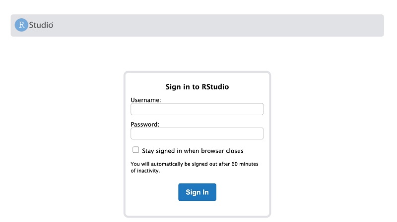
  1. Log in to the RStudio instance with the username ubuntu and password rstudio7862. 

This setup is for demonstration purposes. Using a public-facing EC2 instance and simple login credential is not the best security practice to host your RStudio instance.

You now clone the code repository via the command-line terminal in the RStudio IDE.

  1. Switch to Terminal tab and execute the command:
    git clone https://github.com/aws-samples/amazon-sagemaker-statistical-simulation-rstudio.git

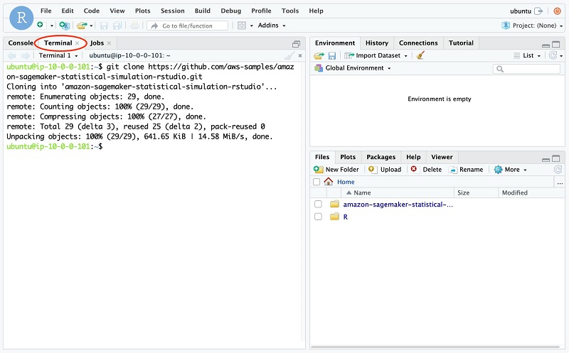
This repository contains the relevant scripts needed to run the simulations and the files to create our Docker container.

Running small simulations locally

On the R console (Console tab), enter the following code to set the working directory to the correct location and install some dependencies:

setwd("~/amazon-sagemaker-statistical-simulation-rstudio/Submit_SageMaker_Processing_Job/")
install.packages(c('doParallel'))

For illustration purposes, we run small simulations on the development machine (the EC2 instance that RStudio is installed on). You can also find the following code in the script Local_Simulation_Commands.R.

On the R Console, we run a very small simulation with 10 iterations:

# takes about: 5.5 seconds
max_iterations <- 10
x_length <- 1000
y_length <- 1000
num_people <- 1000

local_simulation <- 1 # we are running the simulation locally on 1 vCPU
cmd = paste('Rscript Social_Distancing_Simulations.R --args',paste(x_length),paste(y_length), paste(num_people),paste(max_iterations),paste(local_simulation), sep = ' ')
result = system(cmd)

The result is a mean number of 0.11 violations per person, and the time it took to calculate this result was about 5.5 seconds on a t3.xlarge (the precise number of violations per person and time it takes to perform the simulation may vary).

You can play around with running this simulation with different numbers of iterations. Every tenfold increase corresponds to approximately a tenfold increase in the time needed for the simulation. To test this, I ran this simulation with 10,000 iterations, and it finished after 1 hour and 33 minutes. Clearly, a better approach is needed for developers. (If you’re interested in running these, you can find the code in Local_Simulation_Commands.R.)

Building an R container in RStudio IDE and hosting it in Amazon ECR

SageMaker Processing runs your R scripts with a Docker container in a remote compute infrastructure. In this section, we provide an introduction to Docker, how to build a Docker container image, and how to host it in AWS to use in SageMaker Processing.

Docker is a software platform that allows you to build once and deploy applications quickly into any compute environment. Docker packages software into standardized units called containers that have everything the software needs to run, including libraries, system tools, code, and runtime. Docker containers provide isolation and portability for your workload.

A Docker image is a read-only template that defines your container. The image contains the code to run, including any libraries and dependancies your code needs. Docker builds images by reading the instructions from a Dockerfile, which is a text document that contains all the commands you can call on the command line to assemble an image. You can build your Docker images from scratch or base them on other Docker images that you or others have built.

Images are stored in repositories that are indexed and maintained by registries. An image can be pushed into or pulled out of a repository using its registry address, which is similar to a URL. AWS provides Amazon ECR, a fully managed Docker container registry that makes it easy to store, manage, and deploy Docker container images.

Suppose that the Social_Distancing_Simulations.R was originally developed with R 3.4.1 Single Candle from a version of RStudio on ubuntu 16.04. The program uses the library doParallel for parallelism purposes. We want to run the simulation using a remote compute cluster exactly as developed. We need to either install all the dependencies on the remote cluster, which can be difficult to scale, or build a Docker image that has all the dependencies installed in the layers and run it anywhere as a container.

In this section, we create a Docker image that has an R interpreter with dependent libraries to run the simulation and push the image to Amazon ECR so that, with the image, we can run our R script the exact way on any machine that may or may not have the compatible R or the R packages installed, as long as there is a Docker engine on the host system. The following code is the Dockerfile that describes the runtime requirement and how the container should be executed.

#### Dockerfile
FROM ubuntu:16.04

RUN apt-get -y update && apt-get install -y --no-install-recommends 
    wget 
    r-base 
    r-base-dev 
    apt-transport-https 
    ca-certificates

RUN R -e "install.packages(c('doParallel'), repos='https://cloud.r-project.org')"

ENTRYPOINT ["/usr/bin/Rscript"]

Each line is an instruction to create a layer for the image:

  • FROM creates a layer from the ubuntu:16.04 Docker image
  • RUN runs shell command lines to create a new layer
  • ENTRYPOINT allows you configure how a container can be run as an executable

The Dockerfile describes what dependency (ubuntu 16.04, r-base, or doParallel) to include in the container image.

Next, we need to build a Docker image from the Dockerfile, create an ECR repository, and push the image to the repository for later use. The provided shell script build_and_push_docker.sh performs all these actions. In this section, we walk through the steps in the script.

Execute the main script build_and_push_docker.sh that we prepared for you in the terminal:

cd /home/ubuntu/amazon-sagemaker-statistical-simulation-rstudio/
sh build_and_push_docker.sh r_simulation_container v1

The shell script takes two input arguments: a name for the container image and repository, followed by a tag name. You can replace the name r_simulation_container with something else if you want. v1 is the tag of the container, which is the version of the container. You can change that as well. If you do so, remember to change the corresponding repository and image name later.

If all goes well, you should see lots of actions and output indicating that Docker is building and pushing the layers to the repository, followed by a message like the following:

v1: digest: sha256:91adaeb03ddc650069ba8331243936040c09e142ee3cd360b7880bf0779700b1 size: 1573

You may receive warnings regarding storage of credentials. These warnings don’t interfere with pushing the container to ECR, but can be fixed. For more information, see Credentials store.

In the script, the docker build command builds the image and its layers following the instruction in the Dockerfile:

#### In build_and_push_docker.sh
docker build -t $image_name .

The following commands interact with Amazon ECR to create a repository:

#### In build_and_push_docker.sh
# Get the AWS account ID
account=$(aws sts get-caller-identity --query Account --output text)

# Get the region defined in the current configuration (default to us-west-2 if none defined)
region=$(aws configure get region)
region=${region:-us-west-2}

# Define the full image name on Amazon ECR
fullname="${account}.dkr.ecr.${region}.amazonaws.com/${image_name}:${tag}"

# If the repository doesn't exist in ECR, create it.
aws ecr describe-repositories --repository-names "${image_name}" > /dev/null 2>&1

if [ $? -ne 0 ]
then
    aws ecr create-repository --repository-name "${image_name}" > /dev/null
fi

# Get the login command from ECR and execute it directly
aws ecr get-login-password --region ${region} 
  | docker login 
      --username AWS 
      --password-stdin ${account}.dkr.ecr.${region}.amazonaws.com

Finally, the script tags the image and pushes it to the ECR repository:

#### In build_and_push_docker.sh
# Tag and push the local image to Amazon ECR
docker tag ${image_name} ${fullname}
docker push ${fullname}

At this point, we have created a container and pushed it to a repository in Amazon ECR. We can confirm it exists on the Amazon ECR console.

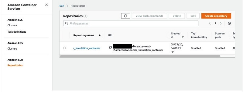
Copy and save the URI for the image; we need it in a later step.

We can use this image repeatedly to run any R scripts that use doParallel. If you have other dependencies, either R native packages that can be downloaded and installed from CRAN (the Comprehensive R Archive Network) with install.packages() or packages that have other runtime dependencies. For instance, RStan, a probabilistic package that implements full Bayesian statistical inference via Markov Chain Monte Carlo that depends on Stan and C++, can be installed into a Docker image by translating their installation instructions in a Dockerfile.

Modifying your R script for SageMaker Processing

Next, we need to modify the existing simulation script so it can talk to the resources available to the running container in the SageMaker Processing compute infrastructure. The resource we need to make the script aware is typically input and output data from S3 buckets. The SageMaker Processing API allows you to specify where the input data is and how it should be mapped to the container so you can access programmatically in the script.

For example, in the following diagram, if you specify the input data s3://bucket/path/to/input_data to be mapped to /opt/ml/processing/input, you can access your input data within the script and container in /opt/ml/processing/input. SageMaker Processing manages the data transfer between the S3 buckets and the container. Similarly, for output, if you need to persist any artifact, you can save the them to /opt/ml/processing/output within the script. The files are then available in the s3://bucket/path/to/output_data.

The only change for the Social_Distancing_Simulations.R script is where the output file gets written to. Instead of a file path on the local EC2 instance, we change it to write to /opt/ml/processing/output/output_result_mean.txt.

Submitting your R script to SageMaker Processing

Very large simulations may be slow on a local machine. As we saw earlier, doing 10,000 iterations of the social distancing simulation takes about 1 hour and 33 minutes on the local machine using 1 vCPU. Now we’re ready to run the simulation with SageMaker Processing.

With SageMaker Processing, we can use the remote compute infrastructure to run the simulation and free up the local compute resources. SageMaker spins up a Processing infrastructure, takes your script, copies your input data from Amazon S3 (if any), and pulls the container image from Amazon ECR to perform the simulation.

SageMaker fully manages the underlying infrastructure for a Processing job. Cluster resources are provisioned for the duration of your job, and cleaned up when a job is complete. The output of the Processing job is stored in the S3 bucket you specified. You can treat your RStudio instance as a launching station to submit simulations to remote compute with various parameters or input datasets.

The complete SageMaker API is accessible through the Reticulate library, which provides an R interface to make calls to the SageMaker Python SDK. To orchestrate these steps, we use another R script.

Copy the following code into the RStudio console. Set the variable container to the URI of the container with the tag (remember to include the tag, and not just the container). It should look like XXXXXXXXXXXX.dkr.ecr.us-west-2.amazonaws.com/r_simulation_container:v1. You can retrieve this URI from the Amazon ECR console by choosing the r_simulation_container repository and copying the relevant URI from the Image URI field (this code is also in the SageMaker_Processing_SDS.R script):

library(reticulate)

use_python('/usr/bin/python') # this is where we installed the SageMaker Python SDK
sagemaker <- import('sagemaker')
session <- sagemaker$Session()
bucket <- session$default_bucket()
role_arn <- sagemaker$get_execution_role()

## using r_container
container <- 'URI TO CONTAINER AND TAG' # can be found under $ docker images. Remember to include the tag

# one single run
processor <- sagemaker$processing$ScriptProcessor(role = role_arn,
                                                  image_uri = container,
                                                  command = list('/usr/bin/Rscript'),
                                                  instance_count = 1L,
                                                  instance_type = 'ml.m5.4xlarge',
                                                  volume_size_in_gb = 5L,
                                                  max_runtime_in_seconds = 3600L,
                                                  base_job_name = 'social-distancing-simulation',
                                                  sagemaker_session = session)

max_iterations <- 10000
x_length <- 1000
y_length <- 1000
num_people <- 1000

is_local <- 0 #we are going to run this simulation with SageMaker processing
result=processor$run(code = 'Social_Distancing_Simulations.R',
              outputs=list(sagemaker$processing$ProcessingOutput(source='/opt/ml/processing/output')),
              arguments = list('--args', paste(x_length), paste(y_length), paste(num_people), paste(max_iterations),paste(is_local)),
              wait = TRUE,
              logs = TRUE)

In the preceding code, we’re off-loading the heavy simulation work to a remote, larger EC2 instance (instance_type = 'ml.m5.4xlarge'). Not only do we not consume any local compute resources, but we also have an opportunity to optimally choose a right-sized instance to perform the simulation on a per-job basis. The machine that we run this simulation on is a general purpose instance with 64 GB RAM and 16 virtual CPUs. The simulation runs faster in the right-sized instance. For example, when we used the ml.m5.4xlarge (64 GB RAM and 16 vCPUs), the simulation took 10.8 minutes. By way of comparison, we performed this exact same simulation on the local development machine using only 1 vCPU and the exact same simulation took 93 minutes.

If you want to run another simulation that is more complex, with more iterations or with a larger dataset, you don’t need to stop and change your EC2 instance type. You can easily change the instance with the instance_type argument to a larger instance for more RAM or virtual CPUs, or to a compute optimized instance, such as ml.c5.4xlarge, for cost-effective high performance at a low price per compute ratio.

We configured our job (by setting wait = TRUE) to run synchronously. The R interpreter is busy until the simulation is complete even though the job is running in a remote compute. In many cases (such as simulations that last many hours) it’s more useful to set wait = FALSE to run the job asynchronously. This allows you to proceed with your script and perform other tasks within RStudio while the heavy-duty simulation occurs via the SageMaker Processing job.

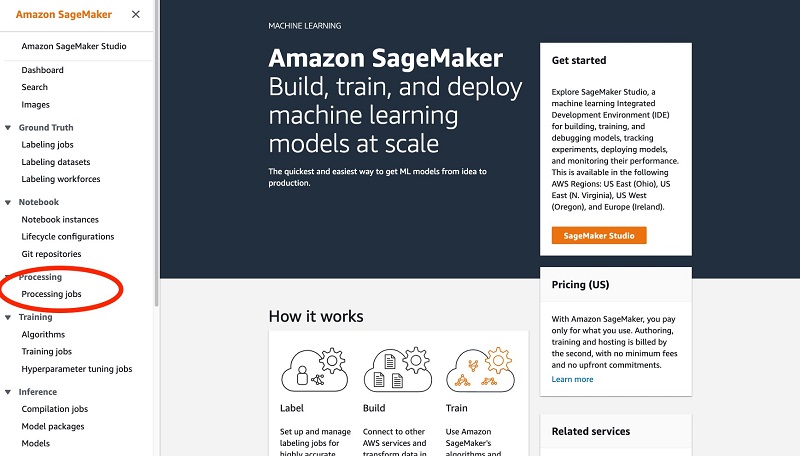
You can inspect and monitor the progress of your jobs on the Processing jobs page on the SageMaker console (you can also monitor jobs via API calls).

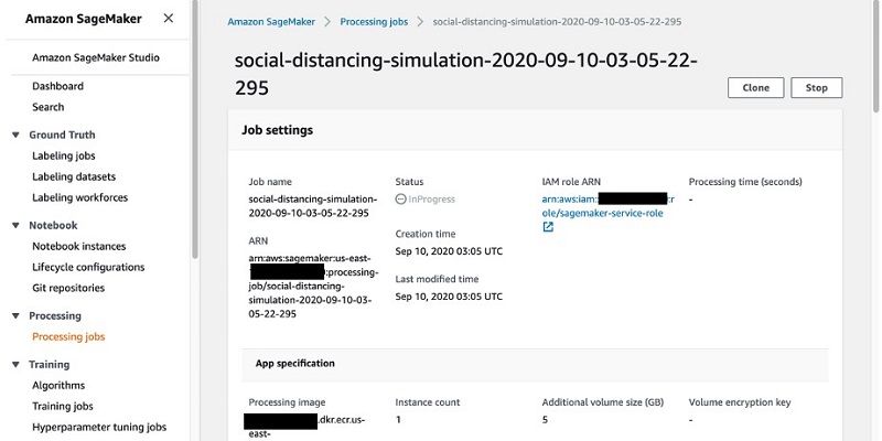
The following screenshot shows the details of our job.

The Monitoring section provides links to Amazon CloudWatch logs for your jobs. This important feature allows you to monitor the logs in near-real time as the job runs, and take necessary action if errors or bugs are detected.


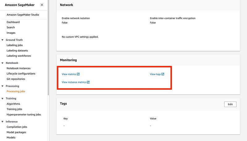
Because logs are reported in near-real time, you don’t have to wait until an entire job is complete to detect problems; you can rely on the emitted logs.

For more information about how SageMaker Processing runs your container image and simulation script, see How Amazon SageMaker Processing Runs Your Processing Container Image.

Accessing simulation results from your R script

Your processing job writes its results to Amazon S3; you can control what is written and in what format it’s written. The Docker container on which the processing job runs writes out the results to the /opt/ml/processing/output directory; this is copied over to Amazon S3 when the processing job is complete. In the Social_Distancing_Simulations.R script, we write the mean of the entire simulation run (this number corresponds to the mean number of violations per person in the room). To access those results, enter the following code (this code is also in SageMaker_Processing_SDS.R script):

get_job_results <- function(session,processor){
    #get the mean results of the simulation
    the_bucket=session$default_bucket()
    job_name=processor$latest_job$job_name
    cmd=capture.output(cat('aws s3 cp s3://',the_bucket,"/",job_name,"/","output/output-1/output_result_mean.txt .",fill = FALSE,sep="")
    )
    system(cmd)
    my_data <- read.delim('output_result_mean.txt',header=FALSE)$V1
    return(my_data)
    }

simulation_mean=get_job_results(session,processor)
cat(simulation_mean) #displays about .11

In the preceding code, we point to the S3 bucket where the results are stored, read the result, and display it. For our use case, our processing job only writes out the mean of the simulation results, but you can configure it to write other values as well.

The following table compares the total time it took us to perform the simulation on the local machine one time, as well as two other instances you can use for SageMaker Processing. For these simulations, the number of iterations changes, but x_length, y_length, and num_people equal 1000 in all cases.

Instance Type
Number of Iterations t3.xlarge (local machine) ml.m5.4xlarge (SageMaker Processing) ml.m5.24xlarge (SageMaker Processing)
10 5.5 (seconds) 254 285
100 87 284 304
1,000 847 284 253
10,000 5602 650 430
100,000 Not Tested Not Tested 1411

For testing on the local machine, we restrict the number of virtual CPUs (vCPU) to 1; the t3.xlarge has 4 vCPUs. This restriction mimics a common pattern in which a large machine is shared by multiple statisticians, and one statistician might not distribute work to multiple CPUs for fear of slowing down their colleagues’ work. For timing for the ml.m5.4xlarge and the ml.m5.24xlarge instances, we use all vCPUs and include the time taken by SageMaker Processing to bring up the requested instance and write the results, in addition to the time required to perform the simulation itself. We perform each simulation one time.

As you can see from the table, local machines are more efficient for fewer iterations, but larger machines using SageMaker Processing are faster when the number of iterations gets to 1,000 or more.

(Optional) Securing your workload in your VPC

So far, we have submitted the SageMaker Processing jobs to a SageMaker managed VPC and accessed the S3 buckets via public internet. However, in healthcare, life science, and financial service industries, it’s usually required to run production workloads in a private VPC with strict networking configuration for security purposes. It’s a security best practice to launch your SageMaker Processing jobs into a private VPC where you can have more control over the network configuration and access the S3 buckets via an Amazon S3 VPC endpoint. For more information and setup instructions, see Give SageMaker Processing Jobs Access to Resources in Your Amazon VPC.

We have provisioned an Amazon S3 VPC endpoint attached to the VPC as part of the CloudFormation template. To launch a job into a private VPC, we need to add the network configuration to an additional argument network_config to the ScriptProcessor construct:

subnet <- 'subnet-xxxxxxx'  # can be found in CloudFormation > Resources
security_group <- 'sg-xxxxxxx'  # can be found in CloudFormation > Resources
network <- sagemaker$network$NetworkConfig(subnets = list(subnet), 
                                           security_group_ids = list(security_group),
                                           enable_network_isolation = TRUE)

processor <- sagemaker$processing$ScriptProcessor(..., network_config = network)

When you run processor$run(...), the SageMaker Processing job is forced to run inside the specified VPC rather than the SageMaker managed VPC, and access the S3 bucket via the Amazon S3 VPC endpoint rather than public internet.

Cleaning up

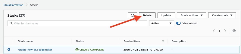
When you complete this post, delete the stack from the AWS CloudFormation console by selecting the stack and choosing Delete. This cleans up all the resources we created for this post.

Conclusion

In this post, we presented a solution using SageMaker Processing as a compute resource extension for R users performing statistical workload on RStudio. You can obtain the scalability you desire with a few lines of code to call the SageMaker API and a reusable Docker container image, without leaving your RStudio IDE. We also showed how you can launch SageMaker Processing jobs into your own private VPC for security purposes.

A question that you might be asking is: Why should the data scientist bother with job submission in the first place? Why not just run RStudio on a very, very large instance that can handle the simulations locally? The answer is that although this is technically possible, it could be expensive, and doesn’t scale to teams of even small sizes. For example, assume your company has 10 statisticians that need to run simulations that use up to 60 GB of RAM; they need to run in aggregate 1,200 total hours (50 straight days) of simulations. If each statistician is provisioned with their own m5.4xlarge instance for 24/7 operation, it costs about 10 * 24 * 30 * $0.768 = $5,529 a month (on-demand Amazon EC2 pricing in us-west-2 as of December 2020). By comparison, provisioning one m5.4xlarge instance to be shared by 10 statisticians to perform exploratory analysis and submit large-scale simulations in SageMaker Processing costs only $553 a month on Amazon EC2, and an additional $1,290 for the 1,200 total hours of simulation on ml.m5.4xlarge SageMaker ML instances ($1.075 per hour).

For more information about R and SageMaker, see the R User Guide to Amazon SageMaker. For details on SageMaker Processing pricing, see the Processing tab on Amazon SageMaker pricing.


About the Authors

Michael Hsieh is a Senior AI/ML Specialist Solutions Architect. He works with customers to advance their ML journey with a combination of AWS ML offerings and his ML domain knowledge. As a Seattle transplant, he loves exploring the great mother nature the city has to offer, such as the hiking trails, scenery kayaking in the SLU, and the sunset at the Shilshole Bay.


Joshua Broyde is an AI/ML Specialist Solutions Architect on the Global Healthcare and Life Sciences team at Amazon Web Services. He works with customers in healthcare and life sciences on a number of AI/ML fronts, including analyzing medical images and video, analyzing machine sensor data and performing natural language processing of medical and healthcare texts.

Read More

Delivering operational insights directly to your on-call team by integrating Amazon DevOps Guru with Atlassian Opsgenie

Delivering operational insights directly to your on-call team by integrating Amazon DevOps Guru with Atlassian Opsgenie

As organizations continue to adopt microservices, the number of disparate services that contribute to delivering applications increases, driving the scope of signals that on-call teams monitor to grow exponentially. It’s becoming more important than ever for these teams to have tools that can quickly and autonomously detect anomalous behaviors across the services they support. Amazon DevOps Guru uses machine learning (ML) to quickly identify when your applications are behaving outside of their normal operating patterns, and may even predict these anomalous behaviors before they become a problem. You can deliver these insights in near-real-time directly to your on-call teams by integrating DevOps Guru with Atlassian Opsgenie, allowing them to immediately react to critical anomalies.

Opsgenie is an alert management solution that ensures critical alerts are delivered to the right person in your on-call team, and includes a preconfigured integration for DevOps Guru. This makes it easy to configure the delivery of notifications from DevOps Guru to Opsgenie via Amazon Simple Notification Service (Amazon SNS) in three simple steps. This post will walk you through configuring the delivery of these notifications.

Configuring DevOps Guru Integration

To start integrating DevOps Guru with Opsgenie, complete the following steps:

  1. On the Opsgenie console, choose Settings.

  1. In the navigation pane, choose Integration list.
  2. Filter the list of built-in integrations by DevOps Guru.

  1. Hover over Amazon DevOps Guru and choose Add.

This integration has been pre-configured with a set of defaults that work for many teams. However, you can also customize the integration settings to meet your needs on the Advanced configuration page.

  1. When you’re ready, assign the integration to a team.
  2. Save a copy of the subscription URL (you will need this later).
  3. Choose Save Integration.

Creating an SNS topic and subscribing Opsgenie

To configure Amazon SNS notifications, complete the following steps:

  1. On the Amazon SNS console, choose Topics.
  2. Choose Create topic.
  3. For Type, select Standard.
  4. For name, enter a name, such as operational-insights.
  5. Leave the default settings as they are or configure them to suit your needs.
  6. Choose Create Topic.
  7. After the topic has been created, scroll down to the Subscriptions section and choose Create subscription.
  8. For Protocol, choose HTTPS.
  9. For Endpoint, enter the subscription URL you saved earlier.
  10. Leave the remaining options as the defaults, or configure them to meet your needs.
  11. Choose Create subscription.

Upon creating the subscription, Amazon SNS sends a confirmation message to your Opsgenie integration, which Opsgenie automatically acknowledges on your behalf.

Opsgenie is now ready to receive notifications from DevOps Guru, and there’s just one thing left to do: configure DevOps Guru to monitor your resources and send notifications to our newly created SNS topic.

Setting up Amazon DevOps Guru

The first time you browse to the DevOps Guru console, you will need to enable DevOps Guru to operate on your account.

  1. On the DevOps Guru console, choose Get Started.

If you have already enabled DevOps Guru, you can add your SNS topic by choosing Settings on the DevOps Guru Console, and then skip to step 3.

  1. Select the Resources you want to monitor (for this post, we chose Analyze all AWS resources in the current AWS account).
  2. For Choose an SNS notification topic, select Select an existing SNS topic.
  3. For Choose a topic in your AWS account, choose the topic you created earlier (operational-insights).
  4. Choose Add SNS topic.
  5. Choose Enable (or Save if you have already enabled the service).

DevOps Guru starts monitoring your resources and learning what’s normal behavior for your applications.

Sample application

For DevOps Guru to have an application to monitor, I use AWS CodeStar to build and deploy a simple web service application using Amazon API Gateway and AWS Lambda. The service simply returns a random number.

After deploying my app, I configure a simple load test to run endlessly, and leave it running for a few hours to allow DevOps Guru to baseline the behavior of my app.

Generating Insights

Now that my app has been running for a while, it’s time to change the behavior of my application to generate an insight. To do this, I deployed a small code change that introduces some random latency and HTTP 5xx errors.

Soon after, Opsgenie sends an alert to my phone, triggered by an insight from DevOps Guru. The following screenshot shows the alert I received in Opsgenie.

From this alert, I can see that there is an anomaly in the latency of my random number service. Choosing the InsightUrl provided in the alert directs me to the DevOps Guru console, where I can start digging into the events and metrics that lead to this insight being generated.

The Relevant events page shows an indicator of the events that occurred in the lead-up to the change in behavior. In my case, the key event was a deployment triggered by the update to the code in the Lambda function.

The DevOps Guru Insights page also provides the pertinent metrics that can be used to further highlight the behavior change—in my case, the duration of my Lambda function and the number of API Gateway 5xx errors had increased.

Resolving the error

Now that I’ve investigated the cause of the anomalous behavior, I resolve it by rolling back the code and redeploying. Shortly after, my application returns to normal behavior. DevOps Guru automatically resolves the insight and sends a notification to Opsgenie, closing the related alert.

To confirm that the application is behaving normally again, I return to the Insights page and check the pertinent metrics, where I can see that they have indeed returned to normal again.

If you plan on testing DevOps Guru in this way, keep in mind that the service learns the behavior of your app over time, and a continual break and fix cycle in your app may eventually be considered normal behavior, no longer generating new insights.

Conclusion

Amazon DevOps Guru continuously analyzes streams of disparate data and monitors thousands of metrics to establish normal application behavior. It’s available now in preview, and the Atlassian Opsgenie integration for Amazon DevOps Guru is also available to use now. Opsgenie centralizes alerts from monitoring, logging, and ITSM tools so Dev and IT Ops teams can stay aware and in control. Opsgenie’s flexible rules engine ensures critical alerts are never missed, and the right person is notified at the right time via email, phone, SMS, or mobile push notifications.

Sign up for the Amazon DevOps Guru preview today and start delivering insights about your applications directly to your on-call teams for immediate investigation and remediation using Opsgenie.


About the Author

Adam Strickland is a Principal Solutions Architect based in Sydney, Australia. He has a strong background in software development across research and commercial organizations, and has built and operated global SaaS applications. Adam is passionate about helping Australian organizations build better software, and scaling their SaaS applications to a global audience.

Read More

Introducing AWS Panorama – Improve your operations with computer vision at the edge

Introducing AWS Panorama – Improve your operations with computer vision at the edge

Yesterday at AWS re:Invent 2020, we announced AWS Panorama, a new machine learning (ML) Appliance and SDK, which allows organizations to bring computer vision (CV) to their on-premises cameras to make automated predictions with high accuracy and low latency. In this post, you learn how customers across a range of industries are using AWS Panorama to improve their operations by automating monitoring and visual inspection tasks.

For many organizations, deriving actionable insights from onsite camera video feeds to improve operations remains a challenge, whether it be increasing manufacturing quality, ensuring safety or operating compliance of their facilities, or analyzing customer traffic in retail locations. To derive these insights, customers must monitor live video of facilities or equipment, or review recorded footage after an incident has occurred, which is manual, error-prone, and difficult to scale.

Customers have begun to take advantage of CV models running in the cloud to automate these visual inspection tasks, but there are circumstances when relying exclusively on the cloud isn’t optimal due to latency requirements or intermittent connectivity. For these reasons, CV processed locally at the edge is needed, which makes the data immediately actionable. Some customers have begun exploring existing capabilities for CV at the edge with enterprise cameras, but find that many cameras lack the capability to perform on-device CV, or offer only simple, hard-coded ML models that can’t be customized or improved over time.

AWS Panorama

AWS Panorama, is an ML Appliance and SDK (software development kit) that enables you to add CV to your existing on-premises cameras or use new AWS Panorama-enabled cameras for edge CV, coming soon from partners like Axis Communications and Basler AG.

With AWS Panorama, you can use CV to help automate costly visual inspection tasks, with the flexibility to bring your own CV models, such as those built with Amazon SageMaker, or use pre-built models from AWS or third parties. AWS Panorama removes the heavy lifting from each step of the CV process by making it easier to use live video feeds to enhance tasks that traditionally required visual inspection and monitoring, like evaluating manufacturing quality, finding bottlenecks in industrial processes, assessing worker safety within your facilities, and analyzing customer traffic in retail stores.

The AWS Panorama Appliance

The AWS Panorama Appliance analyzes video feeds from onsite cameras, acting locally on your data in locations where network connectivity is intermittent, and generates highly accurate ML predictions within milliseconds to improve operations.

The AWS Panorama Appliance, when connected to a network, can discover and connect to existing IP cameras that support the ONVIF standard, and run multiple CV models per stream. Your cameras don’t need any built-in ML or smart capabilities, because the AWS Panorama Appliance provides the ability to add CV to your existing IP cameras.

With an IP62 rating, the AWS Panorama Appliance is dust proof and water resistant, making it appropriate for use in harsh environmental conditions, enabling you to bring CV to where it’s needed in industrial locations.

The AWS Panorama Device SDK

The AWS Panorama Device SDK is a device software stack for CV, sample code, APIs, and tools that will support the NVIDIA Jetson product family and Ambarella CV 2x product line. With the AWS Panorama Device SDK, device manufacturers can build new AWS Panorama-enabled edge devices and smart cameras that run more meaningful CV models at the edge, and offer you a selection of edge devices to satisfy your use cases. For more information, refer to the AWS Panorama SDK page.

Customer stories

In this section, we share the stories of customers who are developing with AWS Panorama to improve manufacturing quality control, retail insights, workplace safety, supply chain efficiency, and transportation and logistics, and are innovating faster with CV at the edge.

Manufacturing and industrial

AWS Panorama can help improve product quality and decrease costs that arise from common manufacturing defects by enabling you to take quick corrective action. With the AWS Panorama Appliance, you can run CV applications at the edge to detect manufacturing anomalies using videos from existing IP camera streams that monitor your manufacturing lines. You can integrate the real-time results with your on-premises systems, facilitate automation, and immediately improve manufacturing processes on factory floors or production lines.

“Many unique components go into each guitar, and we rely upon a skilled workforce to craft each part. With AWS Panorama and help from the Amazon Machine Learning Solutions Lab, we can track how long it takes for an associate to complete each task in the assembly of a guitar so that we’re able to optimize efficiency and track key metrics.”

Michael Spandau, SVP Global IT, Fender.


“For packages at Amazon Fulfillment Centers to be successfully packed in a timely manner, the items must first be inbounded into our structured robotic field via an efficient stow process. Items are stowed individually into different bins within each pod carried by our robotic drive units. Today, we use ML computer vision action detection models deployed on SageMaker (in the cloud) to accurately predict the bin in which each item was placed. AWS Panorama gives us the flexibility to run these same models in real time on edge devices, which opens the door to further optimize the stowing process.”

Joseph Quinlivan, Tech VP, Robotics & Fulfillment, Amazon

Reimagined retail insights

In retail environments, the AWS Panorama Appliance enables you to run multiple, simultaneous CV models on the video feeds from your existing onsite cameras. Applications for retail analytics, such as for people counting, heat mapping, and queue management, can help you get started quickly. With the streamlined management capabilities that AWS Panorama offers, you can easily scale your CV applications to include multiple process locations or stores. This means you can access insights faster and with more accuracy, allowing you to make real-time decisions that create better experiences for your customers.

“We want to use computer vision to better understand consumer needs in our stores, optimize operations, and increase the convenience for our visitors. We plan to use AWS Panorama to deploy different computer vision applications at our stores and experiment over time to strengthen our customer experience and value proposition.”

Ian White, Senior Vice President, Strategic Marketing and Innovation, Parkland


“TensorIoT was founded on the instinct that the majority of the ‘compute’ is moving to the edge and all ‘things’ are becoming smarter. AWS Panorama has made moving computer vision to the edge much easier, and we’ve engaged with Parkland Fuel to use AWS Panorama to gather important retail analytics that will help their business thrive.”

Ravikumar Raghunathan, CEO, TensorIoT


“Pilot.AI solves high-impact problems by developing computationally efficient algorithms to enable pervasive artificial intelligence running at the edge. With AWS Panorama, customers can rapidly add intelligence to their existing IP cameras and begin generating real-time insights on their retail operations using Pilot.AI’s high-performance computer vision models.”

Jon Su, CEO, Pilot AI

Workplace safety

AWS Panorama allows you to monitor workplace safety, get notified immediately about any potential issues or unsafe situations, and take corrective action. AWS Panorama allows you to easily route real-time CV application results to AWS services such as Amazon Simple Storage Service (Amazon S3), Amazon Kinesis Video Streams, or Amazon CloudWatch and gather analytics. This means you can make improved data-based decisions to enhance workplace safety and security for your employees.

“Bigmate is focused on critical risk management solutions that leverage computer vision to help organizations improve workplace health and safety. Whether it’s keeping your people out of the way of hazardous equipment or ensuring they have the proper Personal Protective Equipment (PPE), with AWS Panorama we can rapidly deploy a suite of apps using your existing CCTV cameras that provide real-time notifications to avoid critical events while providing you the data you need to drive a safety-first culture.”

Brett Orr, General Manager Chairman, Bigmate


“Organizations are facing unprecedented demand to transform and secure their physical spaces. With Accenture’s Rhythm.IO, we’re focused on helping customers create maximal situational awareness and safer environments, whether for shopping, travel, or public safety, by fusing together operational data and multi-sensor inputs with computer vision insights from AWS Panorama.”

Matthew Lancaster, Managing Director, Accenture


“Construction zones are dynamic environments. At any given time, you’ve got hundreds of deliveries and subcontractors sharing the site with heavy equipment, and it’s changing every day. INDUS.AI is focused on delivering construction intelligence for general contractors. Computer vision is an especially valuable tool for this because of its ability to handle multiple tasks at once. We are looking forward to delivering real-time insights on jobsite management and safety in a SaaS-like experience for AWS Panorama customers.”

Matt Man, CEO, INDUS.AI

Supply chain efficiency

In manufacturing and assembly environments, AWS Panorama can help provide critical input to supply chain operations by tracking throughput and recognizing bar codes, labels of parts, or completed products. Customers in an assembly plant, for example, might want to use AWS Panorama to automatically identify labels and bar codes of goods received at certain identification points, for automatic booking of goods into a warehouse management system.

“Computer vision helps us innovate and optimize several processes, and the applications are endless. We want to use computer vision to assess the size of trucks coming to our granaries in order to determine the optimal loading dock for each truck. We also want to use computer vision to understand the movement of assets in our plants to remove bottlenecks. AWS Panorama enables all of these solutions with a managed service and edge appliance for deploying and managing a variety of local computer vision applications.”

Victor Caldas, Computer Vision Capability Lead, Cargill


“Every month, millions of trucks enter Amazon facilities, so creating technology that automates trailer loading, unloading, and parking is incredibly important. Amazon’s Middle Mile Product and Technology (MMPT) has begun using AWS Panorama to recognize license plates on these vehicles and automatically expedite entry and exit for drivers. This enables a safe and fast visit to Amazon sites, ensuring faster package delivery for our customers.”

Steve Armato, VP Middle Mile Product and Technology, Amazon

Transportation and logistics

AWS Panorama allows you to process data to improve infrastructure, logistics, and transportation; get notified immediately about any potential issues or unsafe situations; and implement appropriate solutions. AWS Panorama Appliance allows you to easily connect to existing network cameras, process videos right at the edge, and collect metrics for real-time intelligence, while complying with regulatory requirements on data privacy such as processing data locally without storing the videos locally or transmitting videos to the cloud. This means you can get the information needed to provide improved services to your personnel.

“Siemens Mobility has been a leader for seamless, sustainable, and secure transport solutions for more than 160 years. The Siemens ITS Digital Lab is the innovation team in charge of bringing the latest digital advances to the traffic industry, and is uniquely positioned to provide data analytics and AI solutions to public agencies. As cities face new challenges, municipalities have turned to us to innovate on their behalf. Cities would like to understand how to effectively manage their assets and improve congestion and direct traffic. We want to use AWS Panorama to bring computer vision to existing security cameras to monitor traffic and intelligently allocate curbside space, help cities optimize parking and traffic, and improve quality of life for their constituents.”

Laura Sanchez, Innovation Manager, Siemens Mobility ITS Digital Lab


“The Future of Mobility practice at Deloitte is focused on helping supply chain leaders apply advanced technologies to their biggest transportation and logistics challenges. Computer vision is a powerful tool for helping organizations manage, track, and automate the safe movement of goods. AWS Panorama enables our customers to quickly add these capabilities to their existing camera infrastructure. We’re looking forward to using AWS Panorama to provide real-time intelligence on the location and status of shipping containers. We anticipate logistics providers leveraging this important technology throughout their ground operations.”

Scott Corwin, Managing Director, Deloitte Future of Mobility

How to get started

You can improve your business operations with AWS Panorama in three steps:

  1. Identify the process you want to improve with computer vision.
  2. Develop CV models with SageMaker or use pre-built models from AWS or third parties. If you need CV expertise, take advantage of the wealth of experience that the AWS Panorama partners offer.
  3. Get started now with the preview and evaluate, develop, and test your CV applications with the AWS Panorama Appliance Developer Kit.


About the Authors

Banu Nagasundaram is a Senior Product Manager – Technical for AWS Panorama. She helps enterprise customers to be successful using AWS AI/ML services and solves real world business problems. Banu has over 11 years of semiconductor technology experience prior to AWS, working on AI and HPC compute design for datacenter customers. In her spare time, she enjoys hiking and painting.


Jason Copeland is a veteran product leader at AWS with deep experience in machine learning and computer vision at companies including Apple, Deep Vision, and RingCentral. He holds an MBA from Harvard Business School.


Read More

Build sound classification models for mobile apps with Teachable Machine and TFLite

Build sound classification models for mobile apps with Teachable Machine and TFLite

Posted by Khanh LeViet, TensorFlow Developer Advocate

Sound classification is a machine learning task where you input some sound to a machine learning model to categorize it into predefined categories such as dog barking, car horn and so on. There are already many applications of sound classification, including detecting illegal deforestation activities, or detecting sound of humpback whales for better understanding about their natural behaviors.

We are excited to announce that Teachable Machine now allows you to train your own sound classification model and export it in the TensorFlow Lite (TFLite) format. Then you can integrate the TFLite model to your mobile applications or your IoT devices. This is an easy way to quickly get up and running with sound classification, and you can then explore building production models in Python and exporting them to TFLite as a next step.

Model architecture

Timeline chart of of sound classification model

The model that Teachable Machine uses to classify 1-second audio samples is a small convolutional neural network. As the diagram above illustrates, the model receives a spectrogram (2D time-frequency representation of sound obtained through Fourier transform). It first processes the spectrogram with successive layers of 2D convolution (Conv2D) and max pooling layers. The model ends in a number of dense (fully-connected) layers, which are interleaved with dropout layers for the purpose of reducing overfitting during training. The final output of the model is an array of probability scores, one for each class of sound the model is trained to recognize.

You can find a tutorial to train your own sound classifications models using this approach in Python here.

Train a model using your own dataset

There are two ways to train a sound classification model using your own dataset:

  • Simple way: Use Teachable Machine to collect training data and train the model all within your browser without writing a single line of code. This approach is useful for those who want to build a prototype quickly and interactively.
  • Robust way: Record sounds to use as your training dataset in advance then use Python to train and carefully evaluate your model. Of course, his approach is also more automated and repeatable than the simple way.

Train a model using Teachable Machine

Teachable Machine is a GUI tool that allows you to create training dataset and train several types of machine learning models, including image classification, pose classification and sound classification. Teachable Machine uses TensorFlow.js under the hood to train your machine learning model. You can export the trained models in TensorFlow.js format to use in web browsers, or export in TensorFlow Lite format to use in mobile applications or IoT devices.

Here are the steps to train your models:

  1. Go to Teachable Machine website
  2. Create an audio project
  3. Record some sound clips for each category that you want to recognize. You need only 8 seconds of sound for each category.
  4. Start training. Once it has finished, you can test your model on live audio feed.
  5. Export the model in TFLite format.
Teachable machine chart

Train a model using Python

If you have a large training dataset with several hours of sound recording and or than a dozen of categories, then training a sound classification on a web browser will likely take a lot of time. In that case, you can collect the training dataset in advance, convert them to the WAV format and use this Colab notebook (which includes steps to convert the model to TFLite format) to train your sound classification. Google Colab offers a free GPU so that you can significantly speed up your model training.

Deploy the model to Android with TensorFlow Lite

Once you have trained your TensorFlow Lite sound classification model, you can just put it in this Android sample app to try it out. Just follow these steps:

  1. Clone the sample app from GitHub:
    git clone https://github.com/tensorflow/examples.git
  2. Import the sound classification Android app into Android Studio. You can find it in the lite/examples/sound_classification/android folder.
  3. Add your model (both the soundclassifier.tflite and labels.txt) into the src/main/assets folder replacing the example model that is already there.
  4. Build the app and deploy it on an Android device. Now you can classify sound in real time!
UI of TensorFlow Lite using Sound Classifier

To integrate the model into your own app, you can copy the SoundClassifier.kt class from the sample app and the TFLite model you have trained to your app. Then you can use the model as below:

1. Initialize a `SoundClassifier` instance from your `Activity` or `Fragment` class.

var soundClassifier: SoundClassifier
soundClassifier = SoundClassifier(context).also {
it.lifecycleOwner = context
}

2. Start capturing live audio from the device’s microphone and classify in real time:

soundClassifier.start()

3. Receive classification results in real time as a map of human-readable class names and probabilities of the current sound belonging to each particular category.

let labelName = soundClassifier.labelList[0] // e.g. "Clap"
soundClassifier.probabilities.observe(this) { resultMap ->
let probability = result[labelName] // e.g. 0.7
}

What’s next

We are working on an iOS version of the sample app that will be released in a few weeks. We will also extend TensorFlow Lite Model Maker to allow easy training of sound classification in Python. Stay tuned!

Acknowledgements

This project is a joint effort between multiple teams inside Google. Special thanks to:

  • Google Research: Shanqing Cai, Lisie Lillianfeld
  • TensorFlow team: Tian Lin
  • Teachable Machine team: Gautam Bose, Jonas Jongejan
  • Android team: Saryong Kang, Daniel Galpin, Jean-Michel Trivi, Don Turner

Read More