Computer vision is a field of artificial intelligence (AI) that is gaining in popularity and interest largely due to increased access to affordable cloud-based training compute, more performant algorithms, and optimizations for scalable model deployment and inference. However, despite these advances in individual AI and machine learning (ML) domains, simplifying ML pipelines into coherent and observable workflows so they’re more accessible to smaller business units has remained an elusive goal. This is especially true in the agricultural technology space, where computer vision has strong potential for improving production yields through automation, but also in the area of health and safety, where dangerous jobs may be performed by AI rather than human agtech workers. Agricultural applications by AWS customers like sorting produce based on its grade and defects (IntelloLabs, Clarifruit, and Hectre) and proactively targeting pest control measures as early and as efficiently as possible (Bayer Crop Science), are some areas where computer vision shows strong promise.
Although compelling, these applications of machine vision are generally only accessible to larger agricultural enterprises due to the complexity of the train-compile-deploy-infer sequence for specific edge hardware architectures, which introduces a degree of separation between technology and the practitioners that could most benefit from it. In many cases, this disconnect is grounded in a perceived complexity of AI/ML, and the lack of a clear path for its end-to-end application in primary sectors like agriculture, forestry, and horticulture. In most cases, the prospect of hiring a qualified and experienced data scientist to explore opportunities, without the ability for managers and operators to experiment and innovate directly, is both financially and organizationally impractical. At a recent agtech presentation in New Zealand, an executive participant highlighted the lack of an end-to-end AWS computer vision solution as a limiting factor for experimentation, which would be required in order to justify organizational buy-in for more robust technology evaluation.
This post seeks to demystify how AWS AI/ML services work together, and specifically show how you can generate labeled imagery, train machine vision models against that imagery, and deploy custom image recognition models using Amazon Rekognition Custom Labels. You should be able to get up and running with a custom computer vision model within about an hour by following this tutorial, and make more informed judgments for further investment in AI/ML innovation based on data that is relevant to your specific needs.
Training image storage
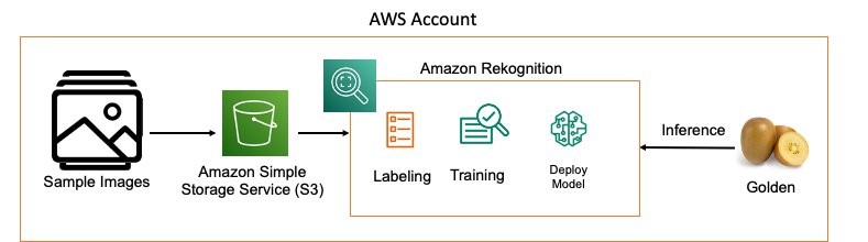
As shown in the following pipeline, the first step to generating a custom computer vision model is to generate labeled images that we use to train our model. To do so, we first load our unlabeled training images into an Amazon Simple Storage Service (Amazon S3) bucket within our account, with each class being stored in its own folder under our bucket. For this example, our prediction classes are two types of kiwifruit (Golden and Monty), with images of known types. After you collect your images of each training class, simply upload them to the respective folder within your Amazon S3 bucket either through the Amazon S3 API or the AWS Management Console.
Setting up Amazon Rekognition
To start using Amazon Rekognition, complete the following steps:
- On the Amazon Rekognition console, choose Use Custom Labels.
- Choose Get started to create a new project.
Projects are used to store your models and training configurations.
- Enter a name for your project (for example,
Kiwifruit-classifier-project). - Choose Create.
- On the Datasets page, choose Create new dataset.
- Enter a name for the dataset (for example,
kiwifruit classifier). - For Image location, select Import images from Amazon S3 bucket.
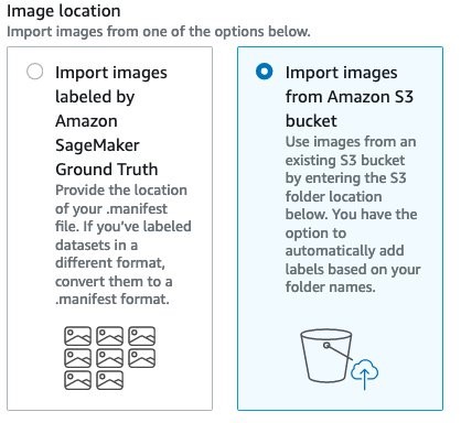
- For S3 folder location, enter the location where your images are stored.
- For Automatic labeling, select Automatically attach a label to my images based on the folder they’re stored in.
This means that the labels of the folders are applied to each image as the class of that image.
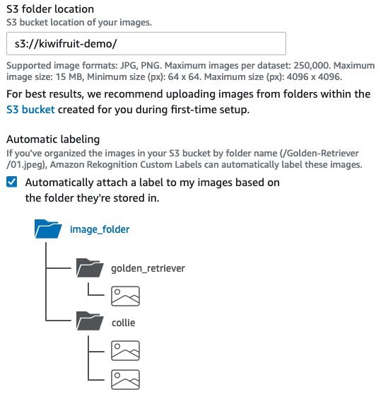
- For Policy, enter the provided JSON into the Amazon S3 bucket, to ensure that Amazon Rekognition can access that data to train the model.

- Choose Submit.
Training the model
Now that we have successfully generated our labeled images using the folder names in which those images are stored, we can train our model.
- Choose Train model to create a project in which our models are stored after training.
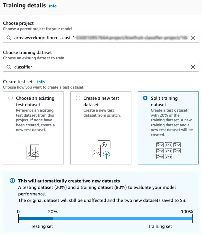
- For Choose project, enter the ARN for the project that you created.
- For Choose a training dataset, choose the dataset you created.
- For Create test set, select Split training dataset.
This automatically reserves part of your labeled data for use in evaluating performance of our trained model.
- Choose Train to start your training job.
Training may take some time (depending on the number of labeled images you provided), and you can monitor progress on the Projects page.
- When training is finished, choose the model under your project to see its performance for each class.
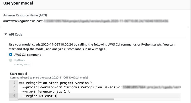
- Under Use your model, choose API Code.
This allows you to get code samples to start and stop your model and conduct inference using the AWS Command Line Interface (AWS CLI).
It can take a few minutes to deploy the inference endpoint after starting the model.
Using your newly trained model
Now that you have a trained model that you’re happy with, using it is as simple as referencing an image from an Amazon S3 bucket using the sample API code provided in order to generate an inference. The following code is an example of Python code using the boto3 library to analyze an image:
client = boto3.client('rekognition',
        region_name='us-east-1',
        aws_access_key_id=access_key_id,
        aws_secret_access_key=access_key
        )

    api_output = client.detect_custom_labels(
        ProjectVersionArn=modelProject,
        Image={
            'S3Object': {
                'Bucket': bucket,
                'Name': 'images/' + filepath
            }
        }
    )
    return api_output
Simply parse the JSON response in order to access the Name and Confidence fields of the payload for the image inference.
Summary
In this post, we learned how to use Amazon Rekognition Custom Labels with an Amazon S3 folder labeling functionality to train an image classification model, deploy that model, and use it to conduct inference. Next steps might be to follow similar steps for a multi-class classifier, or use Amazon SageMaker Ground Truth to generate data with bounding box annotations in addition to class labels. For more information and ideas for other ways to use computer vision in agriculture, check out the AWS Machine Learning Blog and the AWS for Industries: Agriculture Blog.
About the Author
 Steffen Merten is a Startup aligned Principal Solutions Architect based in New Zealand. Prior to AWS, Steffen was Chief Data Officer for Marsello, following five years as an embedded analyst at Palantir. Steffen’s roots are in complex systems analysis with over ten years spent studying both ecological and social systems in the U.S. national security industry throughout the Middle East, South, and Central Asia.


 Graham Zulauf is a Senior Solutions Architect. Graham is focused on helping AWS’ strategic customers solve important problems at scale.
 Huong Nguyen is a Sr. Product Manager at AWS. She is leading the user experience for SageMaker Studio. She has 13 years’ experience creating customer-obsessed and data-driven products for both enterprise and consumer spaces. In her spare time, she enjoys reading, being in nature, and spending time with her family.
 James Sun is a Senior Solutions Architect with Amazon Web Services. James has over 15 years of experience in information technology. Prior to AWS, he held several senior technical positions at MapR, HP, NetApp, Yahoo, and EMC. He holds a PhD from Stanford University.
 Naresh Kumar Kolloju is part of the Amazon SageMaker launch team. He is focused on building secure machine learning platforms for customers. In his spare time, he enjoys hiking and spending time with family.
 Timothy Kwong is a Solutions Architect based out of California. During his free time, he enjoys playing music and doing digital art.
 Praveen Veerath is a Senior AI Solutions Architect for AWS.