Maarek discusses the science behind Alexa Shopping and the newly announced Alexa Prize TaskBot Grand ChallengeRead More
From forecasting demand to ordering – An automated machine learning approach with Amazon Forecast to decrease stockouts, excess inventory, and costs
This post is a guest joint collaboration by Supratim Banerjee of More Retail Limited and Shivaprasad KT and Gaurav H Kankaria of Ganit Inc.
More Retail Ltd. (MRL) is one of India’s top four grocery retailers, with a revenue in the order of several billion dollars. It has a store network of 22 hypermarkets and 624 supermarkets across India, supported by a supply chain of 13 distribution centers, 7 fruits and vegetables collection centers, and 6 staples processing centers.
With such a large network, it’s critical for MRL to deliver the right product quality at the right economic value, while meeting customer demand and keeping operational costs to a minimum. MRL collaborated with Ganit as its AI analytics partner to forecast demand with greater accuracy and build an automated ordering system to overcome the bottlenecks and deficiencies of manual judgment by store managers. MRL used Amazon Forecast to increase their forecasting accuracy from 24% to 76%, leading to a reduction in wastage by up to 30% in the fresh produce category, improving in-stock rates from 80% to 90%, and increasing gross profit by 25%.
We were successful in achieving these business results and building an automated ordering system because of two primary reasons:
- Ability to experiment – Forecast provides a flexible and modular platform through which we ran more than 200 experiments using different regressors and types of models, which included both traditional and ML models. The team followed a Kaizen approach, learning from previously unsuccessful models, and deploying models only when they were successful. Experimentation continued on the side while winning models were deployed.
- Change management – We asked category owners who were used to placing orders using business judgment to trust the ML-based ordering system. A systemic adoption plan ensured that the tool’s results were stored, and the tool was operated with a disciplined cadence, so that in filled and current stock were identified and recorded on time.

Complexity in forecasting the fresh produce category
Forecasting demand for the fresh produce category is challenging because fresh products have a short shelf life. With over-forecasting, stores end up selling stale or over-ripe products, or throw away most of their inventory (termed as shrinkage). If under-forecasted, products may be out of stock, which affects customer experience. Customers may abandon their cart if they can’t find key items in their shopping list, because they don’t want to wait in checkout lines for just a handful of products. To add to this complexity, MRL has many SKUs across its over 600 supermarkets, leading to more than 6,000 store-SKU combinations.
By the end of 2019, MRL was using traditional statistical methods to create forecasting models for each store-SKU combination, which resulted in an accuracy as low as 40%. The forecasts were maintained through multiple individual models, making it computationally and operationally expensive.
Demand forecasting to order placement
In early 2020, MRL and Ganit started working together to further improve the accuracy for forecasting the fresh category, known as Fruits and Vegetables (F&V), and reduce shrinkage.
Ganit advised MRL to break their problem into two parts:
- Forecast demand for each store-SKU combination
- Calculate order quantity (indents)
We go into more detail of each aspect in the following sections.
Forecast demand
In this section, we discuss the steps of forecasting demand for each store-SKU combination.
Understand drivers of demand
Ganit’s team started their journey by first understanding the factors that drove demand within stores. This included multiple on-site store visits, discussions with category managers, and cadence meetings with the supermarket’s CEO coupled with Ganit’s own in-house forecasting expertise on several other aspects like seasonality, stock-out, socio-economic, and macro-economic factors.
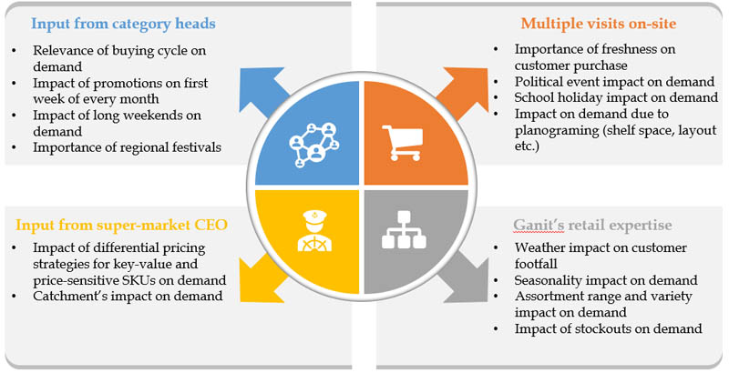
After the store visits, approximately 80 hypotheses on multiple factors were formulated to study their impact on F&V demand. The team performed comprehensive hypotheses testing using techniques like correlation, bivariate and univariate analysis, and statistical significance tests (Student’s t-test, Z tests) to establish the relationship between demand and relevant factors such as festival dates, weather, promotions, and many more.
Data segmentation
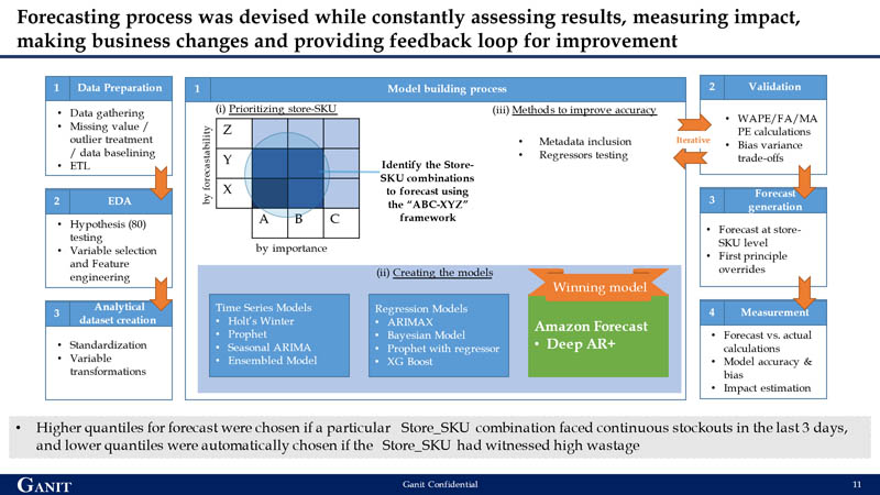
The team emphasized developing a granular model that could accurately forecast a store-SKU combination for each day. A combination of the sales contribution and ease of prediction was built as an ABC-XYZ framework, with ABC indicating the sales contribution (A being the highest) and XYZ indicating the ease of prediction (Z being the lowest). For model building, the first line of focus was on store-SKU combinations that had a high contribution to sales and were the most difficult to predict. This was done to ensure that improving forecasting accuracy has the maximum business impact.
Data treatment
MRL’s transaction data was structured like conventional point of sale data, with fields like mobile number, bill number, item code, store code, date, bill quantity, realized value, and discount value. The team used daily transactional data for the last 2 years for model building. Analyzing historical data helped identity two challenges:
- The presence of numerous missing values
- Some days had extremely high or low sales at bill levels, which indicated the presence of outliers in the data
Missing value treatment
A deep dive into the missing values identified reasons such as no stock available in the store (no supply or not in season) and stores being closed due to planned holiday or external constraints (such as a regional or national shutdown, or construction work). The missing values were replaced with 0, and appropriate regressors or flags were added to the model so the model could learn from this for any such future events.
Outlier treatment
The team treated the outliers at the most granular bill level, which ensured that factors like liquidation, bulk buying (B2B), and bad quality were considered. For example, bill-level treatment may include observing a KPI for each store-SKU combination at a day level, as in the following graph.
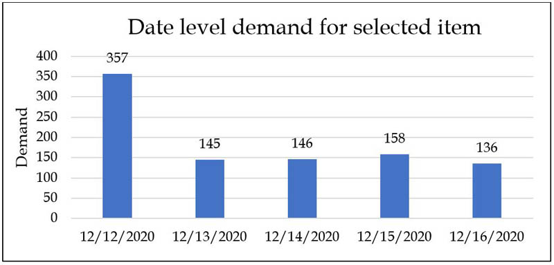
We can then flag dates on which abnormally high quantities are sold as outliers, and dive deeper into those identified outliers. Further analysis shows that these outliers are pre-planned institutional purchases.
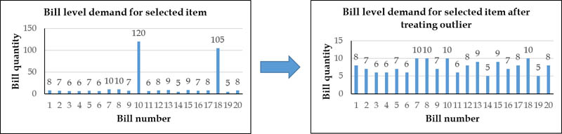
These bill-level outliers are then capped with the maximum sales quantity for that date. The following graphs show the difference in bill-level demand.
Forecasting process
The team tested multiple forecasting techniques like time series models, regression-based models, and deep learning models before choosing Forecast. The primary reason for choosing Forecast was the difference in performance when comparing forecast accuracies in the XY bucket against the Z bucket, which was the most difficult to predict. Although most conventional techniques provided higher accuracies in the XY bucket, only the ML algorithms in Forecast provided a 10% incremental accuracy compared to other models. This was primarily due to Forecast’s ability to learn other SKUs (XY) patterns and apply those learnings to highly volatile items in the Z bucket. Through AutoML, the Forecast DeepAR+ algorithm was the winner and chosen as the forecast model.
Iterating to further improve forecasting accuracy
After the team identified Deep AR+ as the winning algorithm, they ran several experiments with additional features to further improve accuracy. They performed multiple iterations on a smaller sample set with different combinations like pure target time series data (with and without outlier treatment), regressors like festivals or store closures, and store-item metadata (store-item hierarchy) to understand the best combination for improving forecast accuracy. The combination of outlier treated target time series along with store-item metadata and regressors returned the highest accuracy. This was scaled back to the original set of 6,230 store-SKU combinations to get the final forecast.

Order quantity calculation
After the team developed the forecasting model, the immediate next step was to use this to decide how much inventory to buy and place orders. Order generation is influenced by forecasted demand, current stock on hand, and other relevant in-store factors.
The following formula served as the basis for designing the order construct.
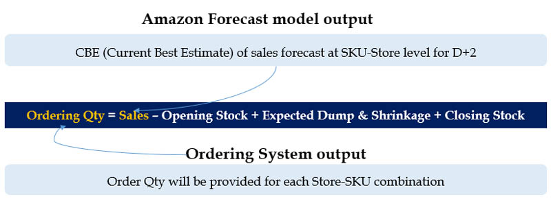
The team also considered other indent adjustment parameters for the automatic ordering system, such as minimum order quantity, service unit factor, minimum closing stock, minimum display stock (based on planogram), and fill rate adjustment, thereby bridging the gap between machine and human intelligence.
Balance under-forecast and over-forecast scenarios
To optimize the output cost of shrinkage with the cost of stockouts and lost sales, the team used the quantiles feature of Forecast to move the forecast response from the model.
In the model design, three forecasts were generated at p40, p50, and p60 quantiles, with p50 being the base quantile. The selection of quantiles was programmed to be based on stockouts and wastage in stores in the recent past. For example, higher quantiles were automatically chosen if a particular store-SKU combination faced continuous stockouts in the last 3 days, and lower quantiles were automatically chosen if the store-SKU had witnessed high wastage. The quantum of increasing and decreasing quantiles was based on the magnitude of stockout or shrinkage within the store.
Automated order placement through Oracle ERP
MRL deployed Forecast and the indent ordering systems in production by integrating them with Oracle’s ERP system, which MRL uses for order placements. The following diagram illustrates the final architecture.
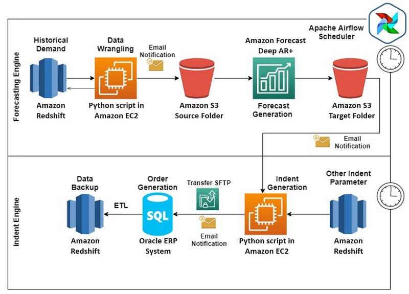
To deploy the ordering system into production, all MRL data was migrated into AWS. The team set up ETL jobs to move live tables to Amazon Redshift (data warehouse for business intelligence work), so Amazon Redshift became the single source of input for future all data processing.
The entire data architecture was divided into two parts:
- Forecasting engine:
- Used historical demand data (1-day demand lag) present in Amazon Redshift
- Other regressor inputs like last bill time, price, and festivals were maintained in Amazon Redshift
- An Amazon Elastic Compute Cloud (Amazon EC2) instance was set up with customized Python scripts to wrangle transaction, regressors, and other metadata
- Post-data wrangling, the data was moved to an Amazon Simple Storage Service (Amazon S3) bucket to generate forecasts (T+2 forecasts for all store-SKU combinations)
- The final forecast output was stored in a separate folder in an S3 bucket
- Order (indent) engine:
- All data required to convert forecasts into orders (such as stock on hand, received to store quantity, last 2 days of orders placed to receive, service unit factor, and planogram-based minimum opening and closing stock) was stored and maintained in Amazon Redshift
- Order quantity was calculated through Python scripts run on EC2 instances
- Orders were then moved to Oracle’s ERP system, which placed an order to vendors
The entire ordering system was decoupled into multiple key segments. The team set up Apache Airflow’s scheduler email notifications for each process to notify respective stakeholders upon successful completion or failure, so that they could take immediate action. The orders placed through the ERP system were then moved to Amazon Redshift tables for calculating the next days’ orders. The ease of integration between AWS and ERP systems led to a complete end-to-end automated ordering system with zero human intervention.
Conclusion
An ML-based approach unlocked the true power of data for MRL. With Forecast, we created two national models for different store formats, as opposed to over 1,000 traditional models that we had been using.
Forecast also learns across time series. ML algorithms within Forecast enable cross-learning between store-SKU combinations, which helps improve forecast accuracies.
Additionally, Forecast allows you to add related time series and item metadata, such as customers who send demand signals based on the mix of items in their basket. Forecast considers all the incoming demand information and arrives at a single model. Unlike conventional models, where the addition of variables leads to overfitting, Forecast enriches the model, providing accurate forecasts based on business context. MRL gained the ability to categorize products based on factors like shelf life, promotions, price, type of stores, affluent cluster, competitive store, and stores throughput. We recommend that you try Amazon Forecast to improve your supply chain operations. You can learn more about Amazon Forecast here. To learn more about Ganit and our solutions, reach out at info@ganitinc.com to learn more.
The content and opinions in this post are those of the third-party author and AWS is not responsible for the content or accuracy of this post.
About the Authors
 Supratim Banerjee is the Chief Transformational Officer at More Retail Limited. He is an experienced professional with a demonstrated history of working in the venture capital and private equity industries. He was a consultant with KPMG and worked with organizations like A.T. Kearney and India Equity Partners. He holds an MBA focused on Finance, General from Indian School of Business, Hyderabad.
 Shivaprasad KT is the Co-Founder & CEO at Ganit Inc. He has a 17+ years of experience in delivering top-line and bottom-line impact using data science in the US, Australia, Asia, and India. He has advised CXOs at companies like Walmart, Sam’s Club, Pfizer, Staples, Coles, Lenovo, and Citibank. He holds an MBA from SP Jain, Mumbai, and a bachelor’s degree in Engineering from NITK Surathkal.
 Gaurav H Kankaria is the Senior Data Scientist at Ganit Inc. He has over 6 years of experience in designing and implementing solutions to help organizations in retail, CPG, and BFSI domains make data-driven decisions. He holds a bachelor’s degree from VIT University, Vellore.
How Latent Space used the Amazon SageMaker model parallelism library to push the frontiers of large-scale transformers
This blog is co-authored by Sarah Jane Hong CSO, Darryl Barnhart CTO, and Ian Thompson CEO of Latent Space and Prem Ranga of AWS.
Latent space is a hidden representation of abstract ideas that machine learning (ML) models learn. For example, “dog,” “flower,” or “door” are concepts or locations in latent space. At Latent Space, we’re working on an engine that allows you to manipulate and explore this space with both language and visual prompts. The Latent Space team comes from two fields that have long had little overlap: graphics and natural language processing (NLP). Traditionally, the modalities of images and text have been handled separately, each with their own history of complex, expensive, and fragile feature engineering. NLP tasks like document understanding or question answering have usually had little in common with vision tasks like scene understanding or rendering, and usually we use very different approaches and models for each task. But this is rapidly changing.
This merging of modalities in a single shared latent space unlocks a new generation of creative and commercial applications, from gaming to document understanding. But unlocking these new applications in a single model opens up new scaling challenges, as highlighted in “The Bitter Lesson” by Richard Sutton, and the exciting work in the last few years on scaling laws. To make this possible, Latent Space is working on cutting-edge research to fuse these modalities in a single model, but also to scale and do so efficiently. This is where model parallelism comes in.
Amazon SageMaker‘s unique automated model partitioning and efficient pipelining approach made our adoption of model parallelism possible with little engineering effort, and we scaled our training of models beyond 1 billion parameters (we use the p4d.24xlarge A100 instances), which is an important requirement for us. Furthermore, we observed that when training with a 16 node, eight GPU training setup with the SageMaker model parallelism library, we recorded a 38% improvement in efficiency compared to our previous training runs.
Challenges with training large-scale transformers
At Latent Space, we’re fusing language and vision in transformer models with billions of parameters to support “out of distribution” use cases from a user’s imagination or that would occur in the real world but not in our training data. We’re handling the challenges inherent in scaling to billions of parameters and beyond in two different ways:
- Retrieval-augmented generation
- The Amazon SageMaker model parallelism library
Information retrieval techniques have long been a key component of search engines and QA tasks. Recently, exciting progress has been made combining classic IR techniques with modern transformers, specifically for question answering tasks where a model is trained jointly with a neural retriever that learns to retrieve relevant documents to help answer questions. For an overview, see the recent work from FAIR in Retrieval Augmented Generation: Streamlining the creation of intelligent natural language processing models and Fusion-in-Decoder, Google Brain’s REALM, and Nvidia’s Neural Retriever for question answering.
While retrieval-augmented techniques help with costs and efficiency, we are still unable to fit the model on a single GPU for our largest model. This means that we need to use model parallelism to train it. However, due to the nature of our retrieval architecture, designing our model splitting was challenging because of interdependencies between retrieved contexts across training inputs. Furthermore, even if we determine how we split our model, introducing model parallelism was a significant engineering task for us to do manually across our research and development lifecycle.
The SageMaker model parallelism library
Model parallelism is the process of splitting a model up between multiple devices or nodes (such as GPU-equipped instances) and creating an efficient pipeline to train the model across these devices to maximize GPU utilization. The model parallelism library in SageMaker makes model parallelism more accessible by providing automated model splitting, also referred to as automated model partitioning and sophisticated pipeline run scheduling. The model splitting algorithms can optimize for speed or memory consumption. The library uses a partitioning algorithm that balances memory, minimizes communication between devices, and optimizes performance.
Automated model partitioning
For our PyTorch use case, the model parallel library internally runs a tracing step (in the first training step) that constructs the model graph and determines the tensor and parameter shapes. It then constructs a tree, which consists of the nested nn.Module objects in the model, as well as additional data gathered from tracing, such as the amount of stored nn.Parameters, and runtime for each nn.Module.
The library then traverses this tree from the root and runs a partitioning algorithm that balances computational load and memory use, and minimizes communication between instances. If multiple nn.Modules share the same nn.Parameter, these modules are placed on the same device to avoid maintaining multiple versions of the same parameter. After the partitioning decision is made, the assigned modules and weights are loaded to their devices.
Pipeline run scheduling
Another core feature of the SageMaker distributed model parallel library is pipelined runs, which determine the order in which computations are made and data is processed across devices during model training. Pipelining is based on splitting a mini-batch into microbatches, which are fed into the training pipeline one by one and follow a run schedule defined by the library runtime.
The microbatch pipeline ensures that all the GPUs are fully utilized, which is something we would have to build ourselves, but with the model parallelism library this happens neatly behind the scenes. Lastly, we can use Amazon FSx, which is important to ensure our read speeds are fast given the number of files being read during the training of a multimodal model with retrieval.
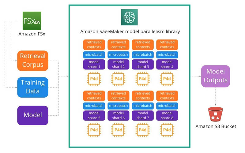
Training architecture
The following diagram represents how we set up our training architecture. Our primary objectives were to improve training speed and reduce costs. The image and language transformers we are training are highly complex, with a significantly large number of layers and weights inside, running to billions of parameters, all of which makes them unable to fit in the memory of a single node. Each node carries a subset of the model, through which the data flows and the transformations are shared and compiled. We setup 16 p4d.24xlarge instances each with eight GPUs using the following architecture representation:
As we scale up our models, a common trend is to have everything stored in the weights of the network. However, for practical purposes, we want to augment our models to learn how to look for relevant contexts to help with the task of rendering. This enables us to keep our serving costs down without compromising on image quality. We use a large transformer-based NLP model and as mentioned before, we observed a 38% increase in training efficiency with the SageMaker model parallelism library as shown by the following:
- We need an allreduce for every computation in the case of tensor level parallelism. This takes O(log_2 n) parallel steps. That is n machines taking O(n) steps, for O(n log_2 n) total operations.
- For pipeline parallelism, we require O(1) parallel steps for passing data down the pipeline
- Given 16 machines with eight GPUs, we have O(1) cost for pipeline parallel, and O(log_2(8)) = O(3) cost for depth-wise model parallel.
- In this case, we see that the network cost is reduced to 1/3rd by switching to pipeline parallel that what we use with SageMaker model parallelism, and the overall training cost reduces to 1/2 + 1/2 * 1/log_2(16) = 0.625 of the original cost leading to a corresponding efficiency improvement.
In general, when the need warrants distributed training (issues with scaling model size or training data), we can follow a set of best practices to determine what approach works best.
Best practices for distributed training
Based on our experience, we suggest starting with a distributed data parallel approach. Distributed data parallelism such as the SageMaker distributed data parallel library resolves most of the networking issues with model replicas, so you should fit models into the smallest number of nodes, then replicate to scale batch size as needed.
If you run out of memory during training, as we did in this scenario, you may want to switch to a model parallel approach. However, consider these alternatives before trying model parallel training:
- On NVIDIA Tensor Core-equipped hardware, use mixed-precision training to create speedup and reduce memory consumption.
- Reduce the batch size (or reduce image resolution or NLP sequence length, if possible).
Additionally, we prefer model designs that do not have batch normalization as described in High-performance large-scale image recognition without normalization. If it cannot be avoided, ensure batch normalization is synced across devices. When you use distributed training, your batch is split across GPUs, so accurate batch statistics require synchronization across all devices. Without this, the normalization will have increased error and thereby impair convergence.
Start with model parallel training when you have the following constraints:
- Your model doesn’t fit on a single device
- Due to your model size, you’re facing limitations in choosing larger batch sizes, such as if your model weights take up most of your GPU memory and you’re forced to choose a smaller, suboptimal batch size
When optimizing for performance, do the following:
- Use pipelining for inter-node communications to minimize latency and increase throughput
- Keep pipelines as short as possible to minimize any bubbles. The number of microbatches should be tuned to balance computational efficiency with bubble size, and be at least the pipeline length. If needed you can form microbatches at the token level as described in TeraPipe: Token Level Pipeline Parallelism for training large-scale language models
When optimizing for cost, use SageMaker managed Spot Instances for training. This can optimize the cost of training models up to 90% over On-Demand instances. SageMaker manages the Spot interruptions on your behalf.
Other factors to consider:
- Within a node when there is a fast interconnect, it’s more nuanced. If there is ample intra-node network capacity, reshuffling data for more optimal compute may show a benefit.
- If activations are much larger than weight tensors, a sharded optimizer may also help. Please refer to ZeRO for more details.
The following table provides some common training scaleup scenarios and how you can configure them on AWS.
| Scenario | When does it apply? | Solution |
| Scaling from a single GPU to many GPUs | When the amount of training data or the size of the model is too large | Change to a multi-GPU instance such as p3.16xlarge, which has eight GPUs, with the data and processing split across the eight GPUs, and producing a near-linear speedup in the time it takes to train your model. |
| Scaling from a single instance to multiple instances | When the scaling needs extend beyond changing the instance size | Scale the number of instances with the SageMaker Python SDK’s estimator function by setting your instance_type to p3.16xlarge and instance_count to 2. Instead of the eight GPUs on a single p3.16xlarge, you have 16 GPUs across two identical instances. Consider using the SageMaker distributed data parallel library. |
| Selecting a model parallel approach for training | When encountering out of memory errors during training | Switch to a model parallel approach using the SageMaker distributed model parallel library. |
| Network performance for inter-node communications | For distributed training with multiple instances (for example, communication between the nodes in the cluster when doing an AllReduce operation) | Your instances need to be in the same Region and same Availability Zone. When you use the SageMaker Python SDK, this is handled for you. Your training data should also be in the same Availability Zone. Consider using the SageMaker distributed data parallel library. |
| Optimized GPU, network, and Storage | For large scale distributed training needs | The p4d.24xlarge instance type was designed for fast local storage and a fast network backplane with up to 400 gigabits, and we highly recommend it as the most performant option for distributed training. |
Conclusion
With the model parallel library in SageMaker, we get a lot of the benefits out of the box, such as automated model partitioning and efficient pipelining. In this post, we shared our challenges with our ML use case, our considerations on different training approaches, and how we used the Amazon SageMaker model parallelism library to speed up our training. Best of all, it can now take only a few hours to adopt best practices for model parallelism and performance improvements described here. If this post helps you or inspires you to solve a problem, we would love to hear about it! Please share your comments and feedback.
References
For more information, please see following:
- Megatron-LM: Training Multi-Billion Parameter Language Models Using Model Parallelism
- Facebook’s blog on retrieval augmented generation architecture.
- Scaling Laws for Autoregressive Generative Modeling
- REALM: Retrieval-Augmented Language Model Pre-Training
- Distilling Knowledge from Reader to Retriever for Question Answering
- High-performance large-scale image recognition without normalization
- TeraPipe: Token Level Pipeline Parallelism for training large-scale language models
- ZeRO: Memory Optimizations Toward Training Trillion Parameter Models
About the Authors
 Prem Ranga is an Enterprise Solutions Architect based out of Atlanta, GA. He is part of the Machine Learning Technical Field Community and loves working with customers on their ML and AI journey. Prem is passionate about robotics, is an autonomous vehicles researcher, and also built the Alexa-controlled Beer Pours in Houston and other locations.
 Sarah Jane Hong is the co-founder and Chief Science Officer at Latent Space. Her background lies at the intersection of human-computer interaction and machine learning. She previously led NLP research at Sonar (acquired by Marchex), which serves businesses in the conversational AI space. She is also an esteemed AR/VR developer, having received awards and fellowships from Oculus, Mozilla Mixed Reality, and Microsoft Hololens.
 Darryl Barnhart is the co-founder and Chief Technology Officer at Latent Space. He is a seasoned developer with experience in GPU acceleration, computer graphics, large-scale data, and machine learning. Other passions include mathematics, game development, and the study of information.
 Ian Thompson is the founder and CEO at Latent Space. Ian is an engineer and researcher inspired by the “adjacent possible” — technologies about to have a big impact on our lives. Currently focused on simplifying and scaling multimodal representation learning to help build safe and creative AI. He previously helped build companies in graphics/virtual reality (AltspaceVR, acquired by Microsoft) and education/NLP (HSE).
LEAF: A Learnable Frontend for Audio Classification
Posted by Neil Zeghidour, Research Scientist, Google Research
Developing machine learning (ML) models for audio understanding has seen tremendous progress over the past several years. Leveraging the ability to learn parameters from data, the field has progressively shifted from composite, handcrafted systems to today’s deep neural classifiers that are used to recognize speech, understand music, or classify animal vocalizations such as bird calls. However, unlike computer vision models, which can learn from raw pixels, deep neural networks for audio classification are rarely trained from raw audio waveforms. Instead, they rely on pre-processed data in the form of mel filterbanks — handcrafted mel-scaled spectrograms that have been designed to replicate some aspects of the human auditory response.
Although modeling mel filterbanks for ML tasks has been historically successful, it is limited by the inherent biases of fixed features: even though using a fixed mel-scale and a logarithmic compression works well in general, we have no guarantee that they provide the best representations for the task at hand. In particular, even though matching human perception provides good inductive biases for some application domains, e.g., speech recognition or music understanding, these biases may be detrimental to domains for which imitating the human ear is not important, such as recognizing whale calls. So, in order to achieve optimal performance, the mel filterbanks should be tailored to the task of interest, a tedious process that requires an iterative effort informed by expert domain knowledge. As a consequence, standard mel filterbanks are used for most audio classification tasks in practice, even though they are suboptimal. In addition, while researchers have proposed ML systems to address these problems, such as Time-Domain Filterbanks, SincNet and Wavegram, they have yet to match the performance of traditional mel filterbanks.
In “LEAF, A Fully Learnable Frontend for Audio Classification”, accepted at ICLR 2021, we present an alternative method for crafting learnable spectrograms for audio understanding tasks. LEarnable Audio Frontend (LEAF) is a neural network that can be initialized to approximate mel filterbanks, and then be trained jointly with any audio classifier to adapt to the task at hand, while only adding a handful of parameters to the full model. We show that over a wide range of audio signals and classification tasks, including speech, music and bird songs, LEAF spectrograms improve classification performance over fixed mel filterbanks and over previously proposed learnable systems. We have implemented the code in TensorFlow 2 and released it to the community through our GitHub repository.
Mel Filterbanks: Mimicking Human Perception of Sound
The first step in the traditional approach to creating a mel filterbank is to capture the sound’s time-variability by windowing, i.e., cutting the signal into short segments with fixed duration. Then, one performs filtering, by passing the windowed segments through a bank of fixed frequency filters, that replicate the human logarithmic sensitivity to pitch. Because we are more sensitive to variations in low frequencies than high frequencies, mel filterbanks give more importance to the low-frequency range of sounds. Finally, the audio signal is compressed to mimic the ear’s logarithmic sensitivity to loudness — a sound needs to double its power for a person to perceive an increase of 3 decibels.
LEAF loosely follows this traditional approach to mel filterbank generation, but replaces each of the fixed operations (i.e., the filtering layer, windowing layer, and compression function) by a learned counterpart. The output of LEAF is a time-frequency representation (a spectrogram) similar to mel filterbanks, but fully learnable. So, for example, while a mel filterbank uses a fixed scale for pitch, LEAF learns the scale that is best suited to the task of interest. Any model that can be trained using mel filterbanks as input features, can also be trained on LEAF spectrograms.
 |
| Diagram of computation of mel filterbanks compared to LEAF spectrograms. |
While LEAF can be initialized randomly, it can also be initialized in a way that approximates mel filterbanks, which have been shown to be a better starting point. Then, LEAF can be trained with any classifier to adapt to the task of interest.
 |
| Left: Mel filterbanks for a person saying “wow”. Right: LEAF’s output for the same example, after training on a dataset of speech commands. |
A Parameter-Efficient Alternative to Fixed Features
A potential downside of replacing fixed features that involve no learnable parameter with a trainable system is that it can significantly increase the number of parameters to optimize. To avoid this issue, LEAF uses Gabor convolution layers that have only two parameters per filter, instead of the ~400 parameters typical of a standard convolution layer. This way, even when paired with a small classifier, such as EfficientNetB0, the LEAF model only accounts for 0.01% of the total parameters.
 |
| Top: Unconstrained convolutional filters after training for audio event classification. Bottom: LEAF filters at convergence after training for the same task. |
Performance
We apply LEAF to diverse audio classification tasks, including recognizing speech commands, speaker identification, acoustic scene recognition, identifying musical instruments, and finding birdsongs. On average, LEAF outperforms both mel filterbanks and previous learnable frontends, such as Time-Domain Filterbanks, SincNet and Wavegram. In particular, LEAF achieves a 76.9% average accuracy across the different tasks, compared to 73.9% for mel filterbanks. Moreover we show that LEAF can be trained in a multi-task setting, such that a single LEAF parametrization can work well across all these tasks. Finally, when combined with a large audio classifier, LEAF reaches state-of-the-art performance on the challenging AudioSet benchmark, with a 2.74 d-prime score.
 |
| D-prime score (the higher the better) of LEAF, mel filterbanks and previously proposed learnable spectrograms on the evaluation set of AudioSet. |
Conclusion
The scope of audio understanding tasks keeps growing, from diagnosing dementia from speech to detecting humpback whale calls from underwater microphones. Adapting mel filterbanks to every new task can require a significant amount of hand-tuning and experimentation. In this context, LEAF provides a drop-in replacement for these fixed features, that can be trained to adapt to the task of interest, with minimal task-specific adjustments. Thus, we believe that LEAF can accelerate development of models for new audio understanding tasks.
Acknowledgements
We thank our co-authors, Olivier Teboul, Félix de Chaumont-Quitry and Marco Tagliasacchi. We also thank Dick Lyon, Vincent Lostanlen, Matt Harvey, and Alex Park for helpful discussions, and Julie Thomas for helping to design figures for this post.

Amazon panel discusses Alexa Prize and other applied science initiatives at WSDM 2021
Watch a recording of the presentation and Q&A roundtable featuring Amazon scientists and scholars.Read More
PDF document pre-processing with Amazon Textract: Visuals detection and removal
Amazon Textract is a fully managed machine learning (ML) service that automatically extracts printed text, handwriting, and other data from scanned documents that goes beyond simple optical character recognition (OCR) to identify, understand, and extract data from forms and tables. Amazon Textract can detect text in a variety of documents, including financial reports, medical records, and tax forms.

In many use cases, you need to extract and analyze documents with various visuals, such as logos, photos, and charts. These visuals contain embedded text that convolutes Amazon Textract output or isn’t required for your downstream process. For example, many real estate evaluation forms or documents contain pictures of houses or trends of historical prices. This information isn’t needed in downstream processes, and you have to remove it before using Amazon Textract to analyze the document. In this post, we illustrate two effective methods to remove these visuals as part of your preprocessing.
Solution overview
For this post, we use a PDF that contains a logo and a chart as an example. We use two different types of processes to convert and detect these visuals, then redact them.
In the first method, we use the OpenCV library canny edge detector to detect the edge of the visuals. For the second method, we write a custom pixel concentration analyzer to detect the location of these visuals.
You can extract these visuals out for further processing, and easily modify the code to fit your use case.

Searchable PDFs are native PDF files usually generated by other applications, such as text processors, virtual PDF printers, and native editors. These types of PDFs retain metadata, text, and image information inside the document. You can easily use libraries like PyMuPDF/fitz to navigate the PDF structure and identify images and text. In this post, we focus on non-searchable or image-based documents.
Option 1: Detecting visuals with OpenCV edge detector
In this approach, we convert the PDF into PNG format, then grayscale the document with the OpenCV-Python library and use the Canny Edge Detector to detect the visual locations. You can follow the detailed steps in the following notebook.

- Convert the document to grayscale.

- Apply the Canny Edge algorithm to detect contours in the Canny-Edged document.
- Identify the rectangular contours with relevant dimensions.

You can further tune and optimize a few parameters to increase detection accuracy depending on your use case:
- Minimum height and width – These parameters define the minimum height and width thresholds for visual detection. It’s expressed in percentage of the page size.
- Padding – When a rectangle contour is detected, we define the extra padding area to have some flexibility on the total area of the page to be redacted. This is helpful in cases where the texts in the visuals aren’t inside clearly delimited rectangular areas.
Advantages and disadvantages
This approach has the following advantages:
- It satisfies most use cases
- It’s easy to implement, and quick to get up and running
- Its optimum parameters yield good results
However, the approach has the following drawbacks:
- For visuals without a bounding box or surrounding edges, the performance may vary depending on the type of visuals
- If a block of text is inside large bounding boxes, the whole text block may be considered a visual and get removed using this logic
Option 2: Pixel concentration analysis
We implement our second approach by analyzing the image pixels. Normal text paragraphs retain a concentration signature in its lines. We can measure and analyze the pixel densities to identify areas with pixel densities that aren’t similar to the rest of document. You can follow the detailed steps in the following notebook.

- Convert the document to grayscale.
- Convert gray areas to white.
- Collapse the pixels horizontally to calculate the concentration of black pixels.
- Split the document into horizontal stripes or segments to identify those that aren’t full text (extending across the whole page).
![]()
- For all horizontal segments that aren’t full text, identify the areas that are text vs. areas that are images. This is done by filtering out sections using minimum and maximum black pixel concentration thresholds.
- Remove areas identified as non-full text.

You can tune the following parameters to optimize the accuracy of identifying non-text areas:
- Non-text horizontal segment thresholds – Define the minimum and maximum black pixel concentration thresholds used to detect non-text horizontal segments in the page.
- Non-text vertical segment thresholds – Define the minimum and maximum black pixel concentration thresholds used to detect non-text vertical segments in the page.
- Window size – Controls how the page is split in horizontal and vertical segments for analysis (X_WINDOW, Y_WINDOW). It’s defined in number of pixels.
- Minimum visual area – Defines the smallest area that can be considered as a visual to be removed. It’s defined in pixels.
- Gray range threshold – The threshold for shades of gray to be removed.
Advantages and disadvantages
This approach is highly customizable. However, it has the following drawbacks:
- Optimum parameters take longer and to achieve a deeper understanding of the solution
- If the document isn’t perfectly rectified (image taken by camera with an angle), this method may fail.
Conclusion
In this post, we showed how you can implement two approaches to redact visuals from different documents. Both approaches are easy to implement. You can get high-quality results and customize either method according to your use case.
To learn more about different techniques in Amazon Textract, visit the public AWS Samples GitHub repo.
About the Authors
 Yuan Jiang is a Sr Solution Architect with a focus in machine learning. He’s a member of the Amazon Computer Vision Hero program and the Amazon Machine Learning Technical Field Community.
 Victor Rojo is a Sr Partner Solution Architect with Conversational AI focus. He’s also a member of the Amazon Computer Vision Hero program.
 Luis Pineda is a Sr Partner Management Solution Architect. He’s also a member of the Amazon Computer Vision Hero program.
 Miguel Romero Calvo is a Data Scientist from the AWS Machine Learning Solution Lab.
Q&A with Brown University’s Anna Lysyanskaya, two-time winner of Facebook research awards in cryptography
In this monthly interview series, we turn the spotlight on members of the academic community and the important research they do — as partners, collaborators, consultants, and independent contributors.
For March, we nominated Anna Lysyanskaya, a professor at Brown University. Lysyanskaya is a two-time Facebook research award recipient in cryptography and is most known for her work in digital signatures and anonymous credentials. In this Q&A, Lysyanskaya shares more about her background, her two winning research proposals, her recent talk at the Real World Cryptography Symposium, and the topics she’s currently focusing on.
Q: Tell us about your role at Brown and the type of research you specialize in.
Anna Lysyanskaya: I am a professor of computer science, and my area of expertise is cryptography, specifically privacy-preserving authentication and anonymous credentials. I’ve had a long career in academia and finished my PhD 19 years ago, so this particular area is something that I started working on basically since I started doing research as a PhD student.
I got into this field mostly by chance, and honestly, I could have ended up anywhere. At the time, everything was new and interesting to me, but I remember I had a chance encounter with the person who would eventually become my adviser. At the time, he had a couple of papers he wanted to take a closer look at, so I started reading them and meeting with him to discuss them.
At the beginning, I was attracted to cryptography because I was interested in the math aspect, as well as the social aspect of solving math problems with interesting people who made everything fun. That initial fascination, paired with being in a great place to study it, led me to where I am today.
Eventually, I learned that it’s not just fun and math, and that there are actually interesting applications of what I’m working on. This is actually why I’m still working on it all this time later, because I just haven’t run out of interesting places to apply this stuff.
Q: You were a winner of two Facebook requests for proposals: the Role of Applied Cryptography in a Privacy-Focused Advertising Ecosystem RFP and the Privacy Preserving Technologies RFP. What were your winning proposals about?
AL: My ads-focused proposal was entitled “Know your anonymous customer.” Let’s start with how a website — say, yourfavoritenewspaper.com — turns content into money: by showing ads. When you click on an ad and buy something, the website that sent you there gets a small payment. At scale, these payments are what pays for the content you find online. The main issue here is that the websites you visit track your activities, and by tracking what you do, they are able to reward the sites that successfully showed you an ad.
My project is about finding a privacy-preserving approach to reward ad publishers — an approach that would not involve tracking a user’s activities but that would still allow reliable accountability when it comes to rewarding a website responsible for sending a customer to, say, a retailer that closed a sale with that customer. The idea is to use anonymous credentials: When you purchase something, your browser obtains a credential from the retailer that just received money from you. Your browser then communicates this credential, transformed in a special way, to whichever website sent you to the original retailer. The crux of the matter is that the transformed credential cannot be linked to the data issued by the retailer, so even if the website and retailer collude, they cannot tell that it was the same user.
My other proposal, which I coauthored with Foteini Baldimtsi from George Mason University, was about private user authentication and anonymous credentials on Facebook’s Libra blockchain. The nature of a blockchain is that it’s very public, but you also want to protect everyone’s privacy, so our goal was to build cryptographic tools for maintaining privacy on the blockchain. Having the opportunity to work with Libra researchers on this project is very exciting.
The tools for both research projects are very similar in spirit, but the stories are different. Because the applications are different enough, you still need to do some original research to solve the problems. The motivations for both projects are achieving user privacy and protecting users.
Q: You recently spoke at Real World Cryptography (RWC). What was your presentation about?
AL: Anonymous credentials have been central to my entire research career. They are what I am most known for, and they were the subject of my talk. An anonymous credential allows you to provide proof that you’re a credentialed user without disclosing any other information. In the aforementioned advertising example, a retail website you visit gives an anonymous credential to your browser that allows you to prove that you have purchased something at this retailer, without revealing who you are or any information that would allow anyone to infer who you are or what you purchased.
Of course, anonymous credentials can be used much more broadly. An especially timely potential application would be vaccination credentials. Suppose that everyone who receives a vaccination also receives a credential attesting to their vaccination status. Then, once you’re vaccinated, you can return to pre-pandemic activities, such as attending concerts and sports events, air travel, and even taking vacation cruises. To gain access to such venues, you’d have to show your vaccination credential. But unless anonymous credentials are used, this is potentially a privacy-invasive proposition, so anonymous credentials are a better approach.
Q: What are some of the biggest research questions you’re interested in?
AL: This talk that I gave at RWC is kind of about this. In a technical field, it’s hard to communicate what you’re doing to people who can actually potentially apply it, mostly because it’s not easy to explain mathematical concepts. Anonymous credentials are especially hard to explain to somebody who hasn’t studied cryptography for at least a few years.
Right now, my focus is to recast this problem in a way that’s a little bit more intuitive. My current attempt is to have an intermediate primitive called a mercurial signature. This is just like a digital signature, but it’s mercurial as in you can transform it in a way that’s still meaningfully signing a statement — just in a way that’s not recognizable to what it looked like when it was first issued.
There are several reasons why I think mercurial signatures are a good building block to study:
- First, we actually do have a candidate construction, so it’s not completely far-fetched, and we know that we can do it. Now, that construction has some shortcomings, but it isn’t a completely crazy idea.
- Second, mercurial signatures are an accessible concept to somebody who has just a basic undergraduate understanding of cryptography. You can actually explain what a mercurial signature is to somebody who knows what a digital signature is in just a few minutes.
- Also, mercurial signatures have very rich applications, and they allow us to build anonymous credentials that have some nice features. One example is delegation. Let’s say I anonymously give a credential to you and then you give a credential to someone else. When they use their credential, it doesn’t reveal what the chain of command is — just that they’re authorized.
This is actually the bulk of my RWC talk, and it’s what I think is the next thing to do.
Q: Where can people learn more about your research?
AL: People can learn more about my research on my Google Scholar profile.
The post Q&A with Brown University’s Anna Lysyanskaya, two-time winner of Facebook research awards in cryptography appeared first on Facebook Research.
GFN Thursday Brings More Support for GOG Version of ‘The Witcher’ Series
Fun fact: Thursday is named for Thor, the hammer-wielding Norse god associated with lightning and thunder. We like to think he’d endorse GFN Thursday as the best day of the week, too.
This is a special Thursday, as we’re happy to share that our cloud-streaming service has added more support for GOG. As part of our continuing open-platform strategy, members who own games from The Witcher series on GOG can now play those versions across their devices. It’s all powered by GeForce NOW’s streaming servers — they’re so powerful that Vikings would have called it magic.
And we’re planning even more events in cooperation with GOG in the future. But first, let’s talk GOG and Geralt.
This Is Your Story
CD PROJEKT RED’s The Witcher series has sold more than 50 million copies, and gamers around the world have joined Geralt on his adventures. Additionally, GOG is a digital distribution platform created with utmost care about customers and we’re big fans of their PC-focused philosophy. They also built GOG GALAXY, an application that combines multiple libraries into one and connects you with friends across all gaming platforms.

We’ve been working with the GOG team to add support for more games ever since the launch of CDPR’s Cyberpunk 2077, the first GOG-enabled game on GFN. With that quest complete, we worked with our partners at GOG on phase two.
That phase begins today. Members who own the following titles on GOG can stream the games across their devices straight from our cloud-gaming servers.
Members can also easily capture their best gameplay moments in The Witcher 3: Wild Hunt – Game of the Year Edition, thanks to GeForce NOW’s sharing tools. Capture your best monster takedowns using our in-game overlay, or apply your signature look using NVIDIA Freestyle. And with Ansel, you can compose the perfect photo of Geralt from any angle of CDPR’s beautiful open world.

More to Play
This week, members can look for the following GeForce NOW library additions, including GOG.com support for games from The Witcher series:
- Thronebreaker: The Witcher Tales (GOG.COM)
- The Witcher Adventure Game (GOG.COM)
- The Witcher 2: Assassins of Kings Enhanced Edition (GOG.COM)
- The Witcher 3: Wild Hunt – Game of the Year Edition (GOG.COM)
- Stronghold: Warlords (new release on Steam)
- Monster Energy Supercross – The Official Videogame 4 (day-and-date release on Steam, March 11)
- Pascal’s Wager: Definitive Edition (day-and-date release on Steam, March 12)
- Uno (Steam)
- Workers & Resources: Soviet Republic (Steam)
With GeForce NOW, there’s always another game to play. We’ll see you next GFN Thursday!
The post GFN Thursday Brings More Support for GOG Version of ‘The Witcher’ Series appeared first on The Official NVIDIA Blog.
Startup Green Lights AI Analytics to Improve Traffic, Pedestrian Safety
For all the attention devoted to self-driving cars, there’s another, often-overlooked, aspect to transportation efficiency and safety: smarter roads.
Derq, a startup operating out of Detroit and Dubai, has developed an AI system that can be installed on intersections and highways. Its AI edge appliance uses NVIDIA GPUs to process video and other data from cameras and radars to predict crashes before they happen and to warn connected road users. It can also understand roadways better, with applications ranging from accurate traffic counts to predicting spots on roads that are most prone to crashes.
Derq CEO and co-founder Georges Aoude says his fascination with automotive safety systems stretches back to long weekend drives with his family to visit relatives. He’d wonder why these fast-moving hunks of metal didn’t collide more often.
Time revealed to him that vehicles frequently do, sometimes to deadly effect. In fact, 1.35 million people around the globe perish in auto accidents every year, and millions more are seriously injured.
“Many of our team members have been touched by deadly road crashes,” said Aoude, who himself has lost two relatives on the roads. “This only makes us more determined to get our technology out there to make roadways safer for all.”
As a scholar at MIT, Aoude worked on autonomous satellites and then drone safety, before doing his Ph.D. work on autonomous vehicles. During his graduate work, he began to envision smart cities that work in tandem with autonomous vehicles, and the seed for Derq was planted. Along the way, he received a patent for AI systems that can predict dangerous behaviors.
Dissecting an Intersection
For its initial use case, Derq zeroed in on intersection and pedestrian safety. It chose to test its technology at a busy downtown street crossing considered one of Detroit’s most dangerous. The intersection had no cameras or radars, so Derq procured those and began its monitoring work.
For the past three years, it’s been capturing and training footage of tens of thousands of vehicles and road users a day, 24/7, at that intersection. In addition to predicted red-light violations and dangerous pedestrian movements, the company has been using that data to refine its AI models. As it monitors more intersections and roadways, Derq is constantly expanding its models. All data is anonymized, and no personal information from road users is ever collected or stored.
Those models can determine which actions have the potential to cause crashes and which don’t, and Derq strives for over 95 percent accuracy. Incidents considered high risk are uploaded to Derq’s GPU cloud instance for further analysis and documentation. Eventually, the system will be able to notify connected and autonomous cars and warn them of impending dangers.
“If the driver detects someone is running a red light, that’s too late,” Aoude said. “If you tell the driver two seconds in advance, they now have the chance to react and avoid the collision.”
The Detroit test demonstrated that the system was able to identify potential crashes effectively. Having seen the technology, the Michigan Department of Transportation has expanded its engagement with Derq, which was recently awarded a federal project to deploy its technology at 65 key intersections along 25 miles of connected roads in the Motor City.
Derq has also been deploying its technology in Dublin, Ohio, a suburb of Columbus, and in Las Vegas, and is running a pilot with California Department of Transportation. It’s in discussions with cities in Florida and Texas, as well as in Canada. Further afield, it’s deployed its systems in Dubai and is working with the road and transport agency there on expanding that deployment as well.
Choosing the Right GPU
Derq’s edge units are equipped with NVIDIA GPUs and hardware acceleration that enable them to process large amounts of internet of things data in real time. It’s developing for a variety of GPUs, including the NVIDIA RTX, T4, and Jetson Nano, AGX Xavier and TX2.
But GPUs are just one part of Derq’s relationship with NVIDIA. As a member of the NVIDIA Inception program for AI startups, Aoude said Derq has had an Inception team visit the company’s Dubai office to provide support such as how to optimize their use of GPUs. They’re also in the process of being incorporated into the NVIDIA Metropolis smart spaces AI platform, which Aoude said “will be a great platform to help us scale.”
The company has focused its product on two main unit sizes. A basic unit runs a single application — think of a box that’s deployed at a pedestrian crosswalk — a perfect pairing for a Jetson AGX Xavier. More elaborate boxes, which run more apps on more camera streams at complex and busy intersections, will rely on the more powerful NVIDIA T4 or RTX GPUs.
Derq will also provide traffic planners and engineers with valuable statistics and intelligence, such as real-time graphs, incident notifications and heatmaps, that can help them assess and improve road safety. The system also can provide forensics for government agencies and insurance companies investigating crashes, an area that the company is exploring with insurance providers.
Going forward, Aoude said Derq plans to scale quickly through partnerships with cities, smart infrastructure, and autonomous vehicle firms so that it can get its technology deployed as widely as possible before autonomous vehicles hit the roadways in large numbers.
“We can’t do it on our own,” he said. “We need forward-thinking cities and collaborative partners, and get ready to scale deployments together, to achieve vision zero – eliminating all road fatalities.”
The post Startup Green Lights AI Analytics to Improve Traffic, Pedestrian Safety appeared first on The Official NVIDIA Blog.
Amazon launches new Alexa Prize TaskBot Challenge
University teams will compete in building agents that can help customers complete complex tasks, like cooking and home improvement. Deadline for university team applications is April 16.Read More