Amazon Machine Learning Research Award recipient utilizes a combination of people and machine learning models to illuminate the planet’s incredible biodiversity.Read More
When French classmates Guillaume Jourdain, Hugo Serrat and Jules Beguerie were looking at applying AI to agriculture in 2014 to form a startup, it was hardly a sure bet.
It was early days for such AI applications, and people said it couldn’t be done. But farmers they spoke with wanted it.
So they rigged together a crude demo to show that a GeForce GPU could run a weed-identification network with a camera. And next thing you know, they had their first customer-investor.
In 2016, the former dorm-mates at École Nationale Supérieure d’Arts et Métiers, in Paris, founded Bilberry. The company today develops weed recognition powered by the NVIDIA Jetson edge AI platform for precision application of herbicides at corn and wheat farms, offering as much as a 92 percent reduction in herbicide usage.
Driven by advances in AI and pressures on farmers to reduce their use of herbicides, weed recognition is starting to see its day in the sun. A bumper crop of AI agriculture companies — FarmWise, SeeTree, Smart Ag and John Deere-owned Blue River — is plowing this field.
Farm Tech 2.0
Early agriculture tech was just scratching the surface of what is possible. Applying infrared, it focused on “the green on brown problem,” in which herbicides were applied uniformly to plants — crops and weeds — versus dirt, blasting all plants, said Serrat, the company’s CTO.
Today, the sustainability race is on to treat “green on green,” or just the weeds near the crop, said Serrat.
“Making the distinction between weeds and crops and act in real time accordingly — this is where everyone is fighting for — that’s the actual holy grail,” he said. “To achieve this requires split-second inference in the field with NVIDIA GPUs running computer vision.”
Losses in corn yields due to ineffective treatment of weeds can run roughly 15 percent to 20 percent, according to Bilberry.
The startup’s customers for smart sprayers include agriculture equipment companies Agrifac, Goldacres, Dammann and Berthoud.
Cutting Back Chemicals
Bilberry deploys its NVIDIA Jetson-powered weed recognition on tractor booms that can span a U.S. football field — about 160 feet. It runs 16 cameras on 16 Jetson TX2 modules and can analyze weeds at 17 frames per second for split-second herbicide squirts while traveling 15 miles per hour.
To achieve this blazing-fast inference performance for rapid recognition of weeds, Bilberry exploited the NVIDIA JetPack SDK for TensorRT optimizations of its algorithms. “We push it to the limits,” said Serrat.
Bilberry tapped into what’s known as INT8 weight quantization, which enables more efficient application of deep learning models, particularly helpful for compact embedded systems in which memory and power restraints rule. This allowed them to harness 8-bit integers instead of floating-point numbers, and moving to integer math in place of floating-point helps reduce memory and computing usage as well as application latency.
Bilberry is a member of NVIDIA Inception, a virtual accelerator program that helps startups in AI and data science get to market faster.
Winners: Environment, Yields
The startup’s smart sprayers can now dramatically reduce herbicide usage by pinpointing treatments. That can make an enormous difference on the runoff of chemicals into the groundwater, the company says. It can also improve plant yields by reducing the friendly fire on crops.
“You need to apply the right amount of herbicides to weeds — if you apply too little, the weed will keep growing and creating new seeds. Bilberry can do this at a rate of 242 acres per hour, with our biggest unit” said Serrat.
The focus on agriculture chemical reduction comes as Europe tightens down on carbon cap limits affecting farmers and as consumers embrace organic foods. U.S. organic produce sales in 2020 increased 14 percent to $8.5 billion from a year ago, according to data from Nielsen.
Potato-Sorting Problem
Bilberry recently launched a potato-sorting application in partnership with Downs. Potatoes are traditionally handled by sorting potatoes moving slowly across a conveyor belt. But it’s difficult for food processors to get the labor, and the monotonous work is hard to stay focused on for hours, causing errors.
“It’s really boring — doing it all day, you become crazy,” said Serrat. “And it’s seasonal, so when they need someone, it’s now, and so they’re always having problems getting enough labor.”
This makes it a perfect task for AI. The startup trained its potato-sorting network to see bad potatoes, green potatoes, cut potatoes, rocks and dirt clods among the good spuds. And applying the Jetson Xavier to this vision task, the AI platform can send a signal to one of the doors at the end of the conveyor belt to only allow good potatoes to pass.
“This is the part I love, to build software that handles something moving and has a real impact,” he said.
Amazon SageMaker is a fully managed service that provides every developer and data scientist with the ability to build, train, and deploy machine learning (ML) models quickly. SageMaker removes the heavy lifting from each step of the ML process to make it easier to develop high-quality ML artifacts. AWS Serverless Application Model (AWS SAM) is an open-source framework for building serverless applications. It provides shorthand syntax to express functions, APIs, databases, event source mappings, steps in AWS Step Functions, and more.
Generally, ML workflows orchestrate and automate sequences of ML tasks. A workflow includes data collection, training, testing, human evaluation of the ML model, and deployment of the models for inference.
For continuous integration and continuous delivery (CI/CD) pipelines, AWS recently released Amazon SageMaker Pipelines, the first purpose-built, easy-to-use CI/CD service for ML. Pipelines is a native workflow orchestration tool for building ML pipelines that takes advantage of direct SageMaker integration. For more information, see Building, automating, managing, and scaling ML workflows using Amazon SageMaker Pipelines.
In this post, I show you an extensible way to automate and deploy custom ML models using service integrations between Amazon SageMaker, Step Functions, and AWS SAM using a CI/CD pipeline.
To build this pipeline, you also need to be familiar with the following AWS services:
AWS CodeBuild – A fully managed continuous integration service that compiles source code, runs tests, and produces software packages that are ready to deploy
AWS CodePipeline – A fully managed continuous delivery service that helps you automate your release pipelines
AWS Lambda – A service that lets you run code without provisioning or managing servers. You pay only for the compute time you consume
Amazon Simple Storage Service (Amazon S3) – An object storage service that offers industry-leading scalability, data availability, security, and performance
AWS Step Functions – A serverless function orchestrator that makes it easy to sequence AWS Lambda functions and multiple AWS services
Solution overview
The solution has two main sections:
Use AWS SAM to create a Step Functions workflow with SageMaker – Step Functions recently announced native service integrations with SageMaker. You can use this feature to train ML models, deploy ML models, test results, and expose an inference endpoint. This feature also provides a way to wait for human approval before the state transitions can progress towards the final ML model inference endpoint’s configuration and deployment.
Deploy the model with a CI/CD pipeline – One of the requirements of SageMaker is that the source code of custom models needs to be stored as a Docker image in an image registry such as Amazon ECR. SageMaker then references this Docker image for training and inference. For this post, we create a CI/CD pipeline using CodePipeline and CodeBuild to build, tag, and upload the Docker image to Amazon ECR and then start the Step Functions workflow to train and deploy the custom ML model on SageMaker, which references this tagged Docker image.
The following diagram describes the general overview of the MLOps CI/CD pipeline.
The workflow includes the following steps:
The data scientist works on developing custom ML model code using their local notebook or a SageMaker notebook. They commit and push changes to a source code repository.
A webhook on the code repository triggers a CodePipeline build in the AWS Cloud.
CodePipeline downloads the source code and starts the build process.
CodeBuild downloads the necessary source files and starts running commands to build and tag a local Docker container image.
CodeBuild pushes the container image to Amazon ECR. The container image is tagged with a unique label derived from the repository commit hash.
CodePipeline invokes Step Functions and passes the container image URI and the unique container image tag as parameters to Step Functions.
Step Functions starts a workflow by initially calling the SageMaker training job and passing the necessary parameters.
SageMaker downloads the necessary container image and starts the training job. When the job is complete, Step Functions directs SageMaker to create a model and store the model in the S3 bucket.
Step Functions starts a SageMaker batch transform job on the test data provided in the S3 bucket.
When the batch transform job is complete, Step Functions sends an email to the user using Amazon Simple Notification Service (Amazon SNS). This email includes the details of the batch transform job and links to the test data prediction outcome stored in the S3 bucket. After sending the email, Step Function enters a manual wait phase.
The email sent by Amazon SNS has links to either accept or reject the test results. The recipient can manually look at the test data prediction outcomes in the S3 bucket. If they’re not satisfied with the results, they can reject the changes to cancel the Step Functions workflow.
If the recipient accepts the changes, an Amazon API Gateway endpoint invokes a Lambda function with an embedded token that references the waiting Step Functions step.
The Lambda function calls Step Functions to continue the workflow.
Step Functions resumes the workflow.
Step Functions creates a SageMaker endpoint config and a SageMaker inference endpoint.
When the workflow is successful, Step Functions sends an email with a link to the final SageMaker inference endpoint.
Use AWS SAM to create a Step Functions workflow with SageMaker
To get started, follow the instructions on GitHub to complete the application setup. Alternatively, you can switch to the terminal and enter the following command:
The code has been broken down into subfolders with the main AWS SAM template residing in path cfn/sam-template.yaml.
The Step Functions workflows are stored in the folder statemachine/mlops.asl.json, and any other Lambda functions used are stored in functions folder.
To start with the AWS SAM template, run the following bash scripts from the root folder:
#Create S3 buckets if required before executing the commands.
S3_BUCKET=bucket-mlops #bucket to store AWS SAM template
S3_BUCKET_MODEL=ml-models   #bucket to store ML models
STACK_NAME=sam-sf-sagemaker-workflow   #Name of the AWS SAM stack
sam build  -t cfn/sam-template.yaml    #AWS SAM build
sam deploy --template-file .aws-sam/build/template.yaml
--stack-name ${STACK_NAME} --force-upload
--s3-bucket ${S3_BUCKET} --s3-prefix sam
--parameter-overrides S3ModelBucket=${S3_BUCKET_MODEL}
--capabilities CAPABILITY_IAM
The sam build command builds all the functions and creates the final AWS CloudFormation template. The sam deploy command uploads the necessary files to the S3 bucket and starts creating or updating the CloudFormation template to create the necessary AWS infrastructure.
When the template has finished successfully, go to the CloudFormation console. On the Outputs tab, copy the MLOpsStateMachineArn value to use later.
The following diagram shows the workflow carried out in Step Functions, using VS Code integrations with Step Functions.
The following JSON based snippet of Amazon States Language describes the workflow visualized in the preceding diagram.
Step Functions process to create the SageMaker workflow
In this section, we discuss the detailed steps involved in creating the SageMaker workflow using Step Functions.
Step Functions uses the commit ID passed by CodePipeline as a unique identifier to create a SageMaker training job. The training job can sometimes take a long time to complete; to wait for the job, you use .sync while specifying the resource section of the SageMaker training job.
When the training job is complete, Step Functions creates a model and saves the model in an S3 bucket.
Step Functions then uses a batch transform step to evaluate and test the model, based on batch data initially provided by the data scientist in an S3 bucket. When the evaluation step is complete, the output is stored in an S3 bucket.
Step Functions then enters a manual approval stage. To create this state, you use callback URLs. To implement this state in Step Functions, use .waitForTaskToken while calling a Lambda resource and pass a token to the Lambda function.
The Lambda function uses Amazon SNS or Amazon Simple Email Service (Amazon SES) to send an email to the subscribed party. You need to add your email address to the SNS topic to receive the accept/reject email while testing.
You receive an email, as in the following screenshot, with links to the data stored in the S3 bucket. This data has been batch transformed using the custom ML model created in the earlier step by SageMaker. You can choose Accept or Reject based on your findings.
If you choose Reject, Step Functions stops running the workflow. If you’re satisfied with the results, choose Accept, which triggers the API link. This link passes the embedded token and type to the API Gateway or Lambda endpoint as request parameters to progress to the next Step Functions step.
See the following Python code:
import json
import boto3
sf = boto3.client('stepfunctions')
def lambda_handler(event, context):
    type= event.get('queryStringParameters').get('type')
    token= event.get('queryStringParameters').get('token')

    if type =='success':
        sf.send_task_success(
        taskToken=token,
        output="{}"
    )
    else:
        sf.send_task_failure(
        taskToken=token

    )


    return {
        'statusCode': 200,
        'body': json.dumps('Responded to Step Function')
    }
Step Functions then creates the final unique SageMaker endpoint configuration and inference endpoint. You can achieve this in Lambda code using special resource values, as shown in the following screenshot.
When the SageMaker endpoint is ready, an email is sent to the subscriber with a link to the API of the SageMaker inference endpoint.
Deploy the model with a CI/CD pipeline
In this section, you use the CI/CD pipeline to deploy a custom ML model.
The pipeline starts its run as soon as it detects updates to the source code of the custom model. The pipeline downloads the source code from the repository, builds and tags the Docker image, and uploads the Docker image to Amazon ECR. After uploading the Docker image, the pipeline triggers the Step Functions workflow to train and deploy the custom model to SageMaker. Finally, the pipeline sends an email to the specified users with details about the SageMaker inference endpoint.
The CloudFormation template deploys a CodePipeline pipeline into your AWS account. The pipeline starts running as soon as code changes are committed to the repo. After the source code is downloaded by the pipeline stage, CodeBuild creates a Docker image and tags it with the commit ID and current timestamp before pushing the image to Amazon ECR. CodePipeline moves to the next stage to trigger a Step Functions step (which you created earlier).
When Step Functions is complete, a final email is generated with a link to the API Gateway URL that references the newly created SageMaker inference endpoint.
Test the workflow
To test your workflow, complete the following steps:
Start the CodePipeline build by committing a code change to the codepipeline-ecr-build-sf-execution/container folder.
On the CodePipeline console, check that the pipeline is transitioning through the different stages as expected.
When the pipeline reaches its final state, it starts the Step Functions workflow, which sends an email for approval.
Approve the email to continue the Step Functions workflow.
When the SageMaker endpoint is ready, you should receive another email with a link to the API inference endpoint.
To test the iris dataset, you can try sending a single data point to the inference endpoint.
Copy the inference endpoint link from the email and assign it to the bash variable INFERENCE_ENDPOINT as shown in the following code, then use the
By sending different data, we get different sets of inference results back.
Clean up
To avoid ongoing charges, delete the resources created in the previous steps by deleting the CloudFormation templates. Additionally, on the SageMaker console, delete any unused models, endpoint configurations, and inference endpoints.
Conclusion
This post demonstrated how to create an ML pipeline for custom SageMaker ML models using some of the latest AWS service integrations.
You can extend this ML pipeline further by adding a layer of authentication and encryption while sending approval links. You can also add more steps to CodePipeline or Step Functions as deemed necessary for your project’s workflow.
The sample files are available in the GitHub repo. To explore related features of SageMaker and further reading, see the following:
Sachin Doshi is a Senior Application Architect working in the AWS Professional Services team. He is based out of New York metropolitan area. Sachin helps customers optimize their applications using cloud native AWS services.
Figure 1. A toy linear regression example illustrating Tilted Empirical Risk Minimization (TERM) as a function of the tilt hyperparameter (t). Classical ERM ((t=0)) minimizes the average loss and is shown in pink. As (t to -infty ) (blue), TERM finds a line of best fit while ignoring outliers. In some applications, these ‘outliers’ may correspond to minority samples that should not be ignored. As (t to + infty) (red), TERM recovers the min-max solution, which minimizes the worst loss. This can ensure the model is a reasonable fit for all samples, reducing unfairness related to representation disparity.
In machine learning, models are commonly estimated via empirical risk minimization (ERM), a principle that considers minimizing the average empirical loss on observed data. Unfortunately, minimizing the average loss alone in ERM has known drawbacks—potentially resulting in models that are susceptible to outliers, unfair to subgroups in the data, or brittle to shifts in distribution. Previous works have thus proposed numerous bespoke solutions for these specific problems.
In contrast, in this post, we describe our work in tilted empirical risk minimization (TERM), which provides a unified view on the deficiencies of ERM (Figure 1). TERM considers a modification to ERM that can be used for diverse applications such as enforcing fairness between subgroups, mitigating the effect of outliers, and addressing class imbalance—all in one unified framework.
What is Tilted ERM (TERM)?
Empirical risk minimization is a popular technique for statistical estimation where the model, (theta in R^d), is estimated by minimizing the average empirical loss over data, ({x_1, dots, x_N}):
$$overline{R} (theta) := frac{1}{N} sum_{i in [N]} f(x_i; theta).$$
Despite its popularity, ERM is known to perform poorly in situations where average performance is not an appropriate surrogate for the problem of interest. In our work (ICLR 2021), we aim to address deficiencies of ERM through a simple, unified framework—tilted empirical risk minimization (TERM). TERM encompasses a family of objectives, parameterized by the hyperparameter (t):
TERM recovers ERM when (t to 0). It also recovers other popular alternatives such as the max-loss ((t to +infty)) and min-loss ((t to -infty)). While the tilted objective used in TERM is not new and is commonly used in other domains,1 it has not seen widespread use in machine learning.
In our work, we investigate tilting by: (i) rigorously studying properties of the TERM objective, and (ii) exploring its utility for a number of ML applications. Surprisingly, we find that this simple and general extension to ERM is competitive with state-of-the-art, problem-specific solutions for a wide range of problems in ML.
TERM: Properties and Interpretations
Given the modifications that TERM makes to ERM, the first question we ask is: What happens to the TERM objective when we vary (t)? Below we explore properties of TERM with varying (t) to better understand the potential benefits of (t)-tilted losses. In particular, we find:
Figure 2. We present a toy problem where there are three samples with individual losses: (f_1, f_2), and (f_3). ERM will minimize the average of the three losses, while TERM aggregates them via exponential tilting parameterized by a family of (t)’s. As (t) moves from (-infty) to (+infty), (t)-tilted losses smoothly move from min-loss to avg-loss to max-loss. The colored dots are optimal solutions of TERM for (t in (-infty, +infty)). TERM is smooth for all finite (t) and convex for positive (t).
TERM with varying (t)’s reweights samples to magnify/suppress outliers (as in Figure 1).
TERM smoothly moves between traditional ERM (pink line), the max-loss (red line), and min-loss (blue line), and can be used to trade-off between these problems.
TERM approximates a popular family of quantile losses (such as median loss, shown in the orange line) with different tilting parameters. Quantile losses have nice properties but can be hard to directly optimize.
Next, we discuss these properties and interpretations in more detail.
Varying (t) reweights the importance of outlier samples
First, we take a closer look at the gradient of the t-tilted loss, and observe that the gradients of the t-tilted objective (widetilde{R}(t; theta)) are of the form:
This indicates that the tilted gradient is a weighted average of the gradients of the original individual losses, and the weights are exponentially proportional to the loss values. As illustrated in Figure 1, for positive values of (t), TERM will thus magnify outliers (samples with large losses), and for negative t’s, it will suppress outliers by downweighting them.
TERM offers a trade-off between the average loss and min-/max-loss
Another perspective on TERM is that it offers a continuum of solutions between the min and max losses. As (t) goes from 0 to (+infty), the average loss will increase, and the max-loss will decrease (going from the pink star to the red star in Figure 2), smoothly trading average-loss for max-loss. Similarly, for (t<0), the solutions achieve a smooth tradeoff between average-loss and min-loss. Additionally, as (t >0) increases, the empirical variance of the losses across all samples also decreases. In the applications below we will see how these properties can be used in practice.
TERM solutions approximate superquantile methods
Finally, we note a connection to another popular variant on ERM: superquantile methods. The (k)-th quantile loss is defined as the (k)-th largest individual loss among all samples, which may be useful for many applications. For example, optimizing for the median loss instead of mean may be desirable for applications in robustness, and the max-loss is an extreme of the quantile loss which can be used to enforce fairness. However, minimizing such objectives can be challenging especially in large-scale settings, as they are non-smooth (and generally non-convex). The TERM objective offers an upper bound on the given quantile of the losses, and the solutions of TERM can provide close approximations to the solutions of the quantile loss optimization problem.
[Note] All discussions above assume that the loss functions belong to generalized linear models. However, we empirically observe competitive performance when applying TERM to broader classes of objectives, including deep neural networks. Please see our paper for full statements and proofs.
TERM Applications
TERM is a general framework applicable to a variety of real-world machine learning problems. Using our understanding of TERM from the previous section, we can consider ‘tilting’ at different hierarchies of the data to adjust to the problem of interest. For instance, one can tilt at the sample level, as in the linear regression toy example. It is also natural to perform tilting at the group level to upweight underrepresented groups. Further, we can tilt at multiple levels to address practical applications requiring multiple objectives. In our work, we consider applying TERM to the following problems:
[positive (t)’s]: handling class imbalance, fair PCA, variance reduction for generalization
[hierarchical tilting with (t_1<0, t_2>0)]: jointly addressing robustness and fairness
For all applications considered, we find that TERM is competitive with or outperforms state-of-the-art, problem-specific tailored baselines. In this post, we discuss three examples on robust classification with (t<0), fair PCA with (t>0), and hierarchical tilting.
Robust classification
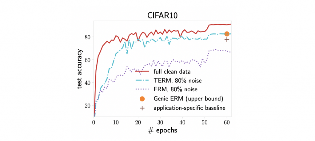
Crowdsourcing is a popular technique for obtaining data labels from a large crowd of annotators. However, the quality of annotators varies significantly as annotators may be unskilled or even malicious. Thus, handling a large amount of noise is essential for the crowdsourcing setting. Here we consider applying TERM ((t<0)) to the application of mitigating noisy annotators.
Specifically, we explore a common benchmark—taking the CIFAR10 dataset and simulating 100 annotators where 20 of them are always correct and 80 of them assign labels uniformly at random. We use negative (t)’s for annotator-level tilting, which is equivalent to assigning annotator-level weights based on the aggregate value of their loss.
Figure 3 demonstrates that our approach performs on par with the oracle method that knows the qualities of annotators in advance. Additionally, we find that the accuracy of TERM alone is 5% higher than that reported by previous approaches which are specifically designed for this problem.
Figure 3. TERM removes the impact of noisy annotators.
Fair principal component analysis (PCA)
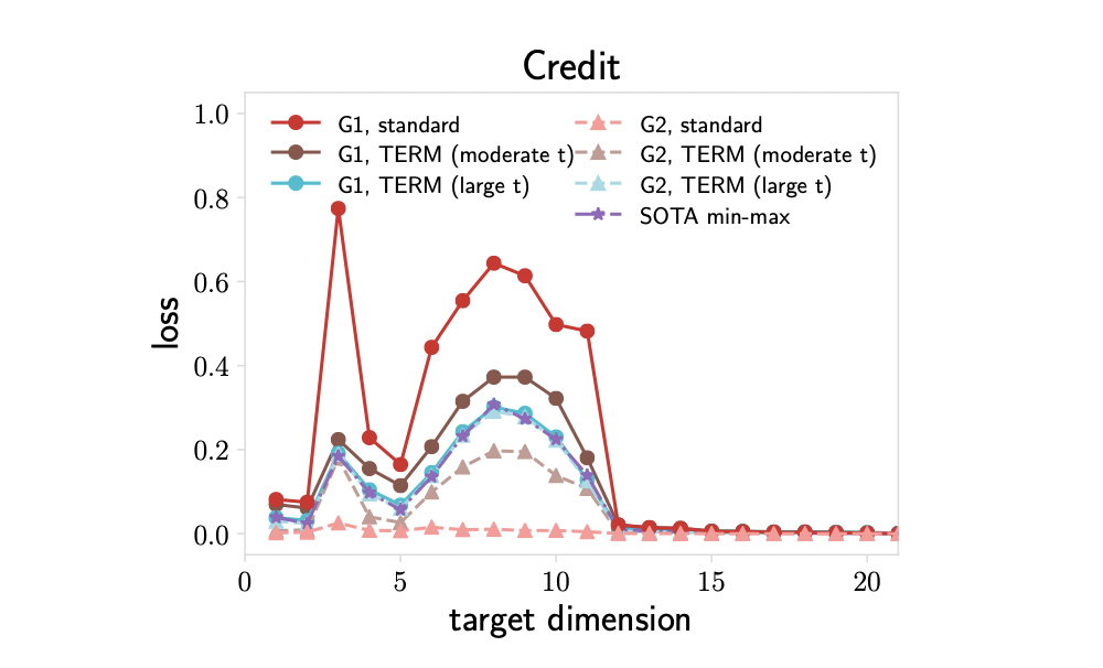
While the previous application explored TERM with (t<0), here we consider an application of TERM with positive (t)’s to fair PCA. PCA is commonly used for dimension reduction while preserving useful information of the original data for downstream tasks. The goal of fair PCA is to learn a projection that achieves similar (or the same) reconstruction errors across subgroups.
Applying standard PCA can be unfair to underrepresented groups. Figure 4 demonstrates that the classical PCA algorithm results in a large gap in the representation quality between two groups (G1 and G2).
To promote fairness, previous methods have proposed to solve a min-max problem via semidefinite programming, which scales poorly with the problem dimension. We apply TERM to this problem, reweighting the gradients based on the loss on each group. We see that TERM with a large (t) can recover the min-max results where the resulting losses on two groups are almost identical. In addition, with moderate values of (t), TERM offers more flexible tradeoffs between performance and fairness by reducing the performance gap less aggressively.
Figure 4. TERM applied to PCA recovers the min-max fair solution with a large t, while offering more flexibility to trade performance on Group 1 (G1) for performance on Group 2 (G2).
Solving compound issues: multi-objective tilting
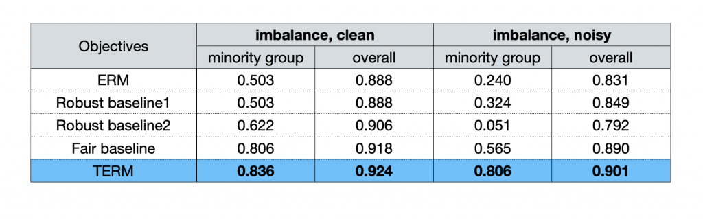
Finally, we note that in practice, multiple issues can co-exist in the data, e.g., we may have issues with both class imbalance and label noise. In these settings we can adopt hierarchical TERM as described previously to address compound issues. Depending on the application, one can choose whether to apply tilting at each level (e.g., possibly more than two levels of hierarchies exist in the data), and at either direction ((t>0) or (t<0)). For example, we can perform negative tilting at the sample level within each group to mitigate outlier samples, and perform positive tilting across all groups to promote fairness.
We test this protocol on the HIV-1 data with logistic regression. In Table 1 below, we find that TERM is superior to all baselines which perform well in their respective problem settings (only showing a subset here) when considering noisy samples and class imbalance simultaneously.
Table 1. Hierarchical TERM can address both class imbalance and noisy samples
More broadly, the idea of tilting can be applied to other learning problems, like GAN training, meta-learning, and improving calibration and generalization for deep learning. We encourage interested readers to view our paper, which explores a more comprehensive set of applications.
[Solving TERM] Wondering how to solve TERM? In our work, we discuss the properties of the objective in terms of its smoothness and convexity behavior. Based on that, we develop both batch and (scalable) stochastic solvers for TERM, where the computation cost is within 2(times) of standard ERM solvers. We describe these algorithms as well as their convergence guarantees in our paper.
Discussion
Our work explores tilted empirical risk minimization (TERM), a simple and general alternative to ERM, which is ubiquitous throughout machine learning. Our hope is that the TERM framework will allow machine learning practitioners to easily modify the ERM objective to handle practical concerns such as enforcing fairness amongst subgroups, mitigating the effect of outliers, and ensuring robust performance on new, unseen data. Critical to the success of such a framework is understanding the implications of the modified objective (i.e., the impact of varying (t)), both theoretically and empirically. Our work rigorously explores these effects—demonstrating the potential benefits of tilted objectives across a wide range of applications in machine learning.
Thanks to Maruan Al-Shedivat, Ahmad Beirami, Virginia Smith, and Ivan Stelmakh for feedback on this blog post.
Footnotes
1 For instance, this type of exponential smoothing (when (t>0)) is commonly used to approximate the max. Variants of tilting have also appeared in other contexts, including importance sampling, decision making, and large deviation theory.
Call it an intellectual Star Wars bar. You could run into just about anything at GTC.
Princeton’s William Tang would speak about using deep learning to unleash fusion energy, UC Berkeley’s Gerry Zhang would talk about hunting for alien signals, Airbus A3’s Arne Stoschek would describe flying autonomous pods.
Want to catch it all? Run. NVIDIA’s GPU Technology Conference has long been almost too much to take in — even if you had fresh sneakers and an employer willing to give you a few days.
But a strange thing happened when this galaxy of astronomers and business leaders and artists and game designers and roboticists went virtual, and free. More people showed up. Suddenly this galaxy of content and connections is anything but far away.
100,000+ Attendees
GTC, which kicks off April 12 with NVIDIA CEO Jensen Huang’s keynote, is a technology conference like no other because it’s not just about technology. It’s about putting technology to work to accelerate what you do, (just about) whatever you do.
We’re expecting more than 100,000 attendees to log into our latest virtual event. We’ve lined up more than 1,500 sessions, and more than 2,200 speakers. That’s more than 1,100 hours of content from 11 industries and in 13 broad topic areas.
There’s no way we could have done this if it wasn’t virtual. And now that it’s entirely virtual — right down to the “Dinner with Strangers” networking event — you can consume as much as want. No sneakers required.
For Business Leaders
Our weeklong event kicks off with a keynote on April 12 at 8:30 a.m. PT from NVIDIA founder and CEO Jensen Huang. It’ll be packed with demos and news.
Following the keynote, you’ll hear from execs at top companies, including Girish Bablani, corporate vice president for Microsoft Azure; Rene Haas, president of Arm’s IP Products Group; Daphne Koller, founder and CEO of Insitro and co-founder of Coursera; Epic Games CTO Kim Libreri; and Hildegard Wortmann, member of the board of management at Audi AG.
They’ll join leaders from Adobe, Amazon, Facebook, GE Renewable Energy, Google, Microsoft, and Salesforce, among many others.
For Developers and Those Early in Their Careers
If you’re just getting started with your career, our NVIDIA Deep Learning Institute will offer nine instructor-led workshops on a wide range of advanced software development topics in AI, accelerated computing and data science.
We also have a track of 101/Getting Started talks from our always popular “Deep Learning Demystified” series. These sessions can help anyone get oriented on the fundamentals of accelerated data analytics, high-level use cases and problem-solving methods — and how deep learning is transforming every industry.
Sessions will be offered live, online, in many time zones and in English, Chinese, Japanese and Korean. Participants can earn an NVIDIA DLI certificate to demonstrate subject-matter competency.
If you’re a technologist, you’ll be able to meet the minds that have created the technologies that have defined our era.
GTC will host three Turing Award winners — Yoshua Bengio, Geoffrey Hinton, Yann LeCun — whose work in deep learning has upended the technological landscape of the 21st century.
GTC will also host nine Gordon Bell winners, people who have brought the power of accelerated computing to bear on the most significant scientific challenges of our time.
Among them are Rommie Amaro, of UC San Diego; Lillian Chong of the University of Pittsburgh; computational biologist Arvind Ramanathan of Argonne National Lab; and James Phillips, a senior research programmer at the University of Illinois.
For Creators and Designers
If you’re an artist, designer or game developer, accelerated computing has long been key to creative industries of all kinds — from architecture to gaming to moviemaking.
Now, with AI, accelerated computing is being woven into the latest art. With our AI Art Gallery, 16 artists will showcase creations developed with AI.
You’ll also have multiple opportunities to participate. Highlights include a live, music-making workshop with the team from Paris-based AIVA and beatboxing sessions with Japanese composer Nao Tokui.
For Entrepreneurs and Investors
If you’re looking to build a new business — or fund one — you’ll find content by the fistfull. Start by loading up your calendar with our four AI Day for VC sessions, April 14.
Then browse sessions spotlighting startups in industries as diverse as healthcare, agriculture, and media and entertainment. Sessions will also touch on regions around the world, including Korean startups driving the self-driving car revolution, Taiwanese healthcare startups and Indian AI startups.
For Networking
While this conference may be virtual, GTC still offers plenty of networking. To connect attendees and speakers from a wide array of backgrounds, we’re continuing our longstanding “Dinner with Strangers” tradition. Attendees will have the opportunity to sit down, over Zoom, with others from their industry.
NVIDIA employee resource communities will host events including Growth for Women in Tech, the Queer in AI Mixer, the Black in AI Mixer and the LatinX in AI Mixer. We’re also launching “AI: Making (X) Better,” a series of talks featuring NVIDIA leaders from underrepresented communities who will discuss their path to AI.
Enough About Us, Make GTC About You
GTC offers an opportunity to engage with groundbreaking technologies like AI-accelerated data centers, deep learning for scientific discoveries, healthcare breakthroughs, next-generation collaboration and more.
Our advice? Register now, it’s free. Block off time in your calendar for the keynote April 12. Then hit the search bar on the conference page and look for content related to what you do — and what interests you.
Suddenly, the conference that’s all about accelerating everything is all about accelerating you.
When freak lightning ignited massive wildfires across Northern California last year, it also sparked efforts from data scientists to improve predictions for blazes.
One effort came from SpaceML, an initiative of the Frontier Development Lab, which is an AI research lab for NASA in partnership with the SETI Institute. Dedicated to open-source research, the SpaceML developer community is creating image recognition models to help advance the study of natural disaster risks, including wildfires.
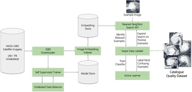
SpaceML uses accelerated computing on petabytes of data for the study of Earth and space sciences, with the goal of advancing projects for NASA researchers. It brings together data scientists and volunteer citizen scientists on projects that tap into the NASA Earth Observing System Data and Information System data. The satellite information came from recorded images of Earth — 197 million square miles — daily over 20 years, providing 40 petabytes of unlabeled data.
“We are lucky to be living in an age where such an unprecedented amount of data is available. It’s like a gold mine, and all we need to build are the shovels to tap its full potential,” said Anirudh Koul, machine learning lead and mentor at SpaceML.
Stoked to Make Difference
Koul, whose day job is a data scientist at Pinterest, said the California wildfires damaged areas near his home last fall. The San Jose resident and avid hiker said they scorched some of his favorite hiking spots at nearby Mount Hamilton. His first impulse was to join as a volunteer firefighter, but instead he realized his biggest contribution could be through lending his data science chops.
Koul enjoys work that helps others. Before volunteering at SpaceML, he led AI and research efforts at startup Aira, which uses augmented reality glasses to dictate for the blind what’s in front of them with image identification paired to natural language processing.
Aira, a member of the NVIDIA Inception accelerator program for startups in AI and data science, was acquired last year.
Inclusive Interdisciplinary Research
The work at SpaceML combines volunteers without backgrounds in AI with tech industry professionals as mentors on projects. Their goal is to build image classifiers from satellite imagery of Earth to spot signs of natural disasters.
Groups take on three-week projects that can examine everything from wildfires and hurricanes to floods and oil spills. They meet monthly with scientists from NASA with domain expertise in sciences for evaluations.
Contributors to SpaceML range from high school students to graduate students and beyond. The work has included participants from Nigeria, Mexico, Korea and Germany and Singapore.
SpaceML’s team members for this project include Rudy Venguswamy, Tarun Narayanan, Ajay Krishnan and Jeanessa Patterson. The mentors are Koul, Meher Kasam and Siddha Ganju, a data scientist at NVIDIA.
Assembling a SpaceML Toolkit
SpaceML provides a collection of machine learning tools. Groups use it to work on such tasks as self-supervised learning using SimCLR, multi-resolution image search, and data labeling, among other tasks. Ease of use is key to the suite of tools.
Among their pipeline of model-building tools, SpaceML contributors rely on NVIDIA DALI for fast preprocessing of data. DALI helps with unstructured data unfit to feed directly into convolutional neural networks to develop classifiers.
“Using DALI we were able to do this relatively quickly,” said Venguswamy.
Findings from SpaceML were published at the Committee on Space Research (COSPAR) so that researchers can replicate their formula.
Classifiers for Big Data
The group developed Curator to train classifiers with a human in the loop, requiring fewer labeled examples because of its self-supervised learning. Curator’s interface is like Tinder, explains Koul, so that novices can swipe left on rejected examples of images for their classifiers or swipe right for those that will be used in the training pipeline.
The process allows them to quickly collect a small set of labeled images and use that against the GIBS Worldview set of the satellite images to find every image in the world that’s a match, creating a massive dataset for further scientific research.
“The idea of this entire pipeline was that we can train a self-supervised learning model against the entire Earth, which is a lot of data,” said Venguswamy.
The CNNs are run on instances of NVIDIA GPUs in the cloud.
To learn more about SpaceML, check out these speaker sessions at GTC 2021:
Fuzz testing is a process of testing APIs with generated data. Fuzzing ensures that code will not break on the negative path, generating randomized inputs that try to cover every branch of code. A popular choice is to pair fuzzers with sanitizers, which are tools that check for illegal conditions and thus flag the bugs triggered by the fuzzers’ inputs.
In this way, fuzzing can find:
Buffer overflows
Memory leaks
Deadlocks
Infinite recursion
Round-trip consistency failures
Uncaught exceptions
And more.
The best way to fuzz to have your fuzz tests running continuously. The more a test runs, the more inputs can be generated and tested against. In this article, you’ll learn how to add a Python fuzzer to TensorFlow.
The technical how-to
TensorFlow Python fuzzers run via OSS-Fuzz, the continuous fuzzing service for open source projects.
For Python fuzzers, OSS-Fuzz uses Atheris, a coverage-guided Python fuzzing engine. Atheris is based on the fuzzing engine libFuzzer, and it can be used with the dynamic memory error detector Address Sanitizer or the fast undefined behavior detector, Undefined Behavior Sanitizer. Atheris dependencies will be pre-installed on OSS-Fuzz base Docker images.
Here is a barebones example of a Python fuzzer for TF. The runtime will call TestCode with different random data.
In the tensorflow repo, in the directory with the other fuzzers, add your own Python fuzzer like above. In TestCode, pick a TensorFlow API that you want to fuzz. In constant_fuzz.py, that API is tf.constant. That fuzzer simply passes data to the chosen API to see if it breaks. No need for code that catches the breakage; OSS-Fuzz will detect and report the bug.
Sometimes an API needs more structured data than just one input. TensorFlow has a Python class called FuzzingHelper that allows you to generate random int lists, a random bool, etc. See an example of its use in sparseCountSparseOutput_fuzz.py, a fuzzer that checks for uncaught exceptions in the API tf.raw_ops.SparseCountSparseOutput.
To build and run, your fuzzer needs a fuzzing target of type tf_py_fuzz_target, defined in tf_fuzzing.bzl. Here is an example fuzz target, with more examples here.
tf_py_fuzz_target(
    name = "fuzz_target_name",
    srcs = ["your_fuzzer.py"],
    tags = ["notap"],  # Important: include to run in OSS.
)
Testing your fuzzer with Docker
Make sure that your fuzzer builds in OSS-Fuzz with Docker.
First install Docker. In your terminal, run command docker image prune to remove any dangling images.
Clone oss-fuzz from Github. The project for a Python TF fuzzer, tensorflow-py, contains a build.sh file to be executed in the Docker container defined in the Dockerfile. Build.sh defines how to build binaries for fuzz targets in tensorflow-py. Specifically, it builds all the Python fuzzers found in $SRC/tensorflow/tensorflow, including your new fuzzer!
The command compile will run build.sh, which will attempt to build your new fuzzer.
The results
Once your fuzzer is up and running, you can search this dashboard for your fuzzer to see what vulnerabilities your fuzzer has uncovered.
Conclusion
Fuzzing is an exciting way to test software from the unhappy path. Whether you want to dabble in security or gain a deeper understanding of TensorFlow’s internals, we hope this post gives you a good place to start.
As mankind bleeds out in the trenches of Enoch, you’ll create your own Outrider and embark on a journey across the hostile planet. Check out this highly anticipated 1-3 player co-op RPG shooter set in an original, dark and desperate sci-fi universe.
Members can also look for the following titles later today:
Narita Boy (day-and-date release on Steam, March 30)
There’s a wide and exciting variety of games coming soon to GeForce NOW:
The Legend of Heroes: Trails of Cold Steel IV (Steam)The long-awaited finale to the epic engulfing a continent comes to a head in the final chapter of the Trails of Cold Steel saga!
The legendary side-scroller is back with beautiful 3D graphics, exhilarating shoot-’em-up gameplay, and a multitude of stages, ships and weapons that will allow you to conduct a symphony of destruction upon your foes.
Play as an adorable yet trouble-making turnip. Avoid paying taxes, solve plantastic puzzles, harvest crops and battle massive beasts all in a journey to tear down a corrupt vegetable government!
And that’s not all — check out even more games you’ll be able to stream from the cloud in April:


 Sachin Doshi is a Senior Application Architect working in the AWS Professional Services team. He is based out of New York metropolitan area. Sachin helps customers optimize their applications using cloud native AWS services.