As companies welcome more autonomous robots and other heavy equipment into the workplace, we need to ensure equipment can operate safely around human teammates. In this post, we will show you how to build a virtual boundary with computer vision and AWS DeepLens, the AWS deep learning-enabled video camera designed for developers to learn machine learning (ML). Using the machine learning techniques in this post, you can build virtual boundaries for restricted areas that automatically shut down equipment or sound an alert when humans come close.
For this project, you will train a custom object detection model with Amazon SageMaker and deploy the model to an AWS DeepLens device. Object detection is an ML algorithm that takes an image as input and identifies objects and their location within the image. In addition to virtual boundary solutions, you can apply techniques learned in this post when you need to detect where certain objects are inside an image or count the number of instances of a desired object in an image, such as counting items in a storage bin or on a retail shelf.
Solution overview
The walkthrough includes the following steps:
- Prepare your dataset to feed into an ML algorithm.
- Train a model with Amazon SageMaker.
- Test model with custom restriction zones.
- Deploy the solution to AWS DeepLens.
We also discuss other real-world use cases where you can apply this solution.
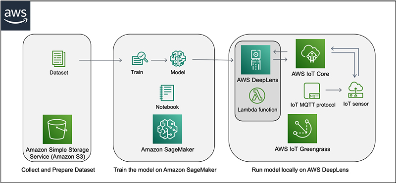
The following diagram illustrates the solution architecture.
Prerequisites
To complete this walkthrough, you must have the following prerequisites:
Prepare your dataset to feed into an ML algorithm
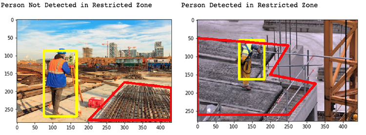
This post uses an ML algorithm called an object detection model to build a solution that detects if a person is in a custom restricted zone. You use the publicly available Pedestrian Detection dataset available on Kaggle, which has over 2,000 images. This dataset has labels for human and human-like objects (like mannequins) so the trained model can more accurately distinguish between real humans and cardboard props or statues.
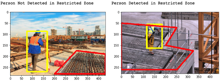
For example, the following images are examples of a construction worker being detected and if they are in the custom restriction zone (red outline).
To start training your model, first create an S3 bucket to store your training data and model output. For AWS DeepLens projects, the S3 bucket names must start with the prefix deeplens-. You use this data to train a model with SageMaker, a fully managed service that provides the ability to build, train, and deploy ML models quickly.
Train a model with Amazon SageMaker
You use SageMaker Jupyter notebooks as the development environment to train the model. Jupyter Notebook is an open-source web application that allows you to create and share documents that contain live code, equations, visualizations, and narrative text. For this post, we provide Train_Object_Detection_People_DeepLens.ipynb, a full notebook for you to follow along.
To create a custom object detection model, you need to use a graphic processing unit (GPU)-enabled training job instance. GPUs are excellent at parallelizing computations required to train a neural network. Although the notebook itself is a single ml.t2.medium instance, the training job specifically uses an ml.p2.xlarge instance. To access a GPU-enabled training job instance, you must submit a request for a service limit increase to the AWS Support Center.
After you receive your limit increase, complete the following steps to create a SageMaker notebook instance:
- On the SageMaker console, choose Notebook instances.
- Choose Create notebook instance.
- For Notebook instance name, enter a name for your notebook instance.
- For Instance type, choose t2.medium.
This is the least expensive instance type that notebook instances support, and it suffices for this tutorial.
- For IAM role, choose Create a new role.
Make sure this AWS Identity and Access Management (IAM) role has access to the S3 bucket you created earlier (prefix deeplens-).
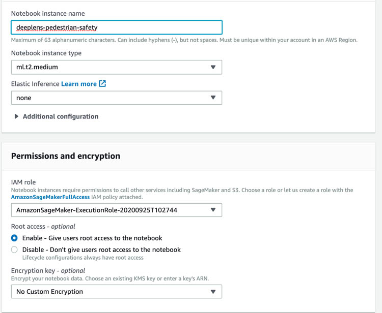
- Choose Create notebook instance. Your notebook instance can take a couple of minutes to start up.
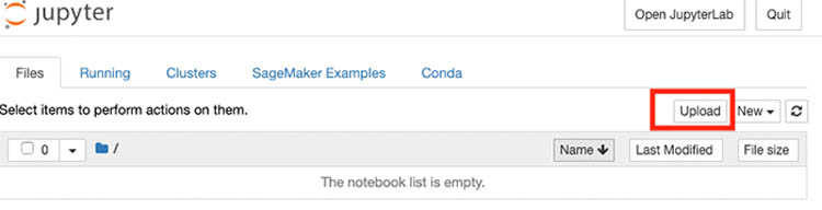
- When the status on the notebook instances page changes to InService, choose Open Jupyter to launch your newly created Jupyter notebook instance.
- Choose Upload to upload the
Train_Object_Detection_people_DeepLens.ipynb file you downloaded earlier.
- Open the notebook and follow it through to the end.
- If you’re asked about setting the kernel, select conda_mxnet_p36.
The Jupyter notebook contains a mix of text and code cells. To run a piece of code, choose the cell and press Shift+Enter. While the cell is running, an asterisk appears next to the cell. When the cell is complete, an output number and new output cell appear below the original cell.
- Download the dataset from the public S3 bucket into the local SageMaker instance and unzip the data. This can be done by following the code in the notebook:
 !aws s3 cp s3://deeplens-public/samples/pedestriansafety/humandetection_data.zip .

!rm -rf humandetection/
!unzip humandetection_data.zip -d humandetection
- Convert the dataset into a format (RecordIO) that can be fed into the SageMaker algorithm:
 !python $mxnet_path/tools/im2rec.py --pass-through --pack-label $DATA_PATH/train_mask.lst $DATA_PATH/
!python $mxnet_path/tools/im2rec.py --pass-through --pack-label $DATA_PATH/val_mask.lst $DATA_PATH/
- Transfer the RecordIO files back to Amazon S3.
Now that you’re done with all the data preparation, you’re ready to train the object detector.
There are many different types of object detection algorithms. For this post, you use the Single-Shot MultiBox Detection algorithm (SSD). The SSD algorithm has a good balance of speed vs. accuracy, making it ideal for running on edge devices such as AWS DeepLens.
As part of the training job, you have a lot of options for hyperparameters that help configure the training behavior (such as number of epochs, learning rate, optimizer type, and mini-batch size). Hyperparameters let you tune training speed and accuracy of your model. For more information about hyperparameters, see Object Detection Algorithm.
- Set up your hyperparameters and data channels. Consider using the following example definition of hyperparameters:
 od_model = sagemaker.estimator.Estimator(training_image,
                                         role,
                                         train_instance_count=1,
                                         train_instance_type='ml.p2.xlarge',
                                         train_volume_size = 50,
                                         train_max_run = 360000,
                                         input_mode= 'File',
                                         output_path=s3_output_location,
                                         sagemaker_session=sess)

od_model.set_hyperparameters(base_network='resnet-50',
                             use_pretrained_model=1,
                             num_classes=2,
                             mini_batch_size=32,
                             epochs=100,
                             learning_rate=0.003,
                             lr_scheduler_step='3,6',
                             lr_scheduler_factor=0.1,
                             optimizer='sgd',
                             momentum=0.9,
                             weight_decay=0.0005,
                             overlap_threshold=0.5,
                             nms_threshold=0.45,
                             image_shape=300,
                             num_training_samples=n_train_samples)
The notebook has some default hyperparameters that have been pre-selected. For pedestrian detection, you train the model for 100 epochs. This training step should take approximately 2 hours using one ml.p2.xlarge instance. You can experiment with different combinations of the hyperparameters, or train for more epochs for performance improvements. For information about the latest pricing, see Amazon SageMaker Pricing.
- You can start a training job with a single line of code and monitor the accuracy over time on the SageMaker console:
od_model.fit(inputs=data_channels, logs=True)
For more information about how training works, see CreateTrainingJob. The provisioning and data downloading take time, depending on the size of the data. Therefore, it might be a few minutes before you start getting data logs for your training jobs.
You can monitor the progress of your training job through the metric mean average precision (mAP), which allows you to monitor the quality of the model’s ability to classify objects and detect the correct bounding boxes. The data logs also print out the mAP on the validation data, among other losses, for every run of the dataset, one time for one epoch. This metric is a proxy for the quality of the algorithm’s performance on accurately detecting the class and the accurate bounding box around it.
When the job is finished, you can find the trained model files in the S3 bucket and folder specified earlier in s3_output_location:
s3_output_location = 's3://{}/{}/output'.format(BUCKET, PREFIX)
For this post, we show results on the validation set at the completion of the 10th epoch and the 100th epoch. At the end of the 10th epoch, we see a validation mAP of approximately 0.027, whereas the 100th epoch was approximately 0.42.
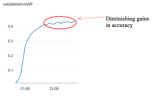
To achieve better detection results, you can try to tune the hyperparameters by using the capability built into SageMaker for automatic model tuning and train the model for more epochs. You usually stop training when you see a diminishing gain in accuracy.
Test model with custom restriction zones
Before you deploy the trained model to AWS DeepLens, you can test it in the cloud by using a SageMaker hosted endpoint. A SageMaker endpoint is a fully managed service that allows you to make real-time inferences via a REST API. SageMaker allows you to quickly deploy new endpoints to test your models so you don’t have to host the model on the local instance that was used to train the model. This allows you to make predictions (or inference) from the model on images that the algorithm didn’t see during training.
You don’t have to host on the same instance type that you used to train. Training is a prolonged and compute-heavy job that requires a different set of compute and memory requirements that hosting typically doesn’t. You can choose any type of instance you want to host the model. In this case, we chose the ml.p3.2xlarge instance to train, but we choose to host the model on the less expensive CPU instance, ml.m4.xlarge. The following code snippet shows our endpoint deployment.
object_detector = od_model.deploy(initial_instance_count = 1,
                                  instance_type = 'ml.m4.xlarge')
Detection in a custom restriction zone (region of interest)
The format of the output can be represented as [class_index, confidence_score, xmin, ymin, xmax, ymax]. Low-confidence predictions often have higher chances of a false positive or false negative, so you should probably discard low-confidence predictions. You can use the following code to detect if the bounding box of the person overlaps with the restricted zone.
def inRestrictedSection(ImShape = None, R1 = None, restricted_region = None, kclass = None, score = None, threshold = None):
    statement = 'Person Not Detected in Restricted Zone'
    if (kclass == 1) and (score > threshold):
        Im1 = np.zeros((ImShape[0],ImShape[1],3), np.int32)
        cv2.fillPoly(Im1, [R1], 255)
        Im2 = np.zeros((ImShape[0],ImShape[1],3), np.int32)
        if restricted_region is None:
            restricted_region = np.array([[0,ImShape[0]],[ImShape[1],ImShape[0]],[ImShape[1],0], [0,0]], np.int32)
        cv2.fillPoly(Im2, [restricted_region], 255)
        Im = Im1 * Im2
        if np.sum(np.greater(Im, 0))>0:
            statement = 'Person Detected in Restricted Zone'
    else:
        statement = statement

    return statement
By default, the complete frame is evaluated for human presence. However, you can easily specify the region of interest within which the presence of a person is deemed as high risk. If you want to add a custom restriction zone, add coordinates of the vertices of the region represented by [X-axis,Y-axis] and create the polygon. The coordinates must be entered in either clockwise or counter-clockwise. See the following code:
restricted_region = None
#restricted_region = np.array([[0,200],[100,200],[100,0], [10,10]], np.int32)
The following sample code shows pedestrians that are identified within a restricted zone:
file_name = 'humandetection/test_images/t1_image.jpg'
img = cv2.imread(file_name)
img =cv2.cvtColor(img,cv2.COLOR_BGR2RGB)
thresh = 0.2
height = img.shape[0]
width = img.shape[1]
colors = dict()


with open(file_name, 'rb') as image:
    f = image.read()
    b = bytearray(f)
    ne = open('n.txt','wb')
    ne.write(b)


results = object_detector.predict(b, initial_args={'ContentType': 'image/jpeg'})
detections = json.loads(results)

object_categories = ['no-person', 'person']

for det in detections['prediction']:
    (klass, score, x0, y0, x1, y1) = det
    if score < thresh:
        continue
    cls_id = int(klass)
    prob = score
    if cls_id not in colors:
        colors[cls_id] = (random.random(), random.random(), random.random())
    xmin = int(x0 * width)
    ymin = int(y0 * height)
    xmax = int(x1 * width)
    ymax = int(y1 * height)

    R1 = np.array([[xmin,ymin],[xmax,ymin],[xmax,ymax], [xmin,ymax]], np.int32)
    cv2.polylines(img,[R1],True, (255,255,0), thickness = 5)
    cv2.polylines(img,[restricted_region],True, (255,0,0), thickness = 5)

    plt.imshow(img)

    print(inRestrictedSection(img.shape,R1 = R1, restricted_region= restricted_region, kclass = cls_id, score = prob, threshold=0.2))
The following images show our results.
Deploy the solution to AWS DeepLens
Convert the model for deployment to AWS DeepLens
When deploying a SageMaker-trained SSD model to AWS DeepLens, you must first run deploy.py to convert the model artifact into a deployable model:
!rm -rf incubator-mxnet
!git clone -b v1.7.x https://github.com/apache/incubator-mxnet

MODEL_PATH = od_model.model_data
TARGET_PATH ='s3://'+BUCKET+'/'+PREFIX+'/patched/'
!rm -rf tmp && mkdir tmp

rm -rf tmp && mkdir tmp
!aws s3 cp $MODEL_PATH tmp
!tar -xzvf tmp/model.tar.gz -C tmp
!mv tmp/model_algo_1-0000.params tmp/ssd_resnet50_300-0000.params
!mv tmp/model_algo_1-symbol.json tmp/ssd_resnet50_300-symbol.json
!python incubator-mxnet/example/ssd/deploy.py --network resnet50 --data-shape 300 --num-class 2 --prefix tmp/ssd_
!tar -cvzf ./patched_model.tar.gz -C tmp ./deploy_ssd_resnet50_300-0000.params ./deploy_ssd_resnet50_300-symbol.json ./hyperparams.json
!aws s3 cp patched_model.tar.gz $TARGET_PATH
Import your model into AWS DeepLens
To run the model on an AWS DeepLens device, you need to create an AWS DeepLens project. Start by importing your model into AWS DeepLens.
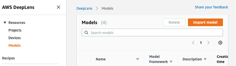
- On the AWS DeepLens console, under Resources, choose Models.
- Choose Import model.
- For Import source, select Externally trained model.
- Enter the Amazon S3 location of the patched model that you saved from running deploy.py in the step above.
- For Model framework, choose MXNet.
- Choose Import model.
Create the inference function
The inference function feeds each camera frame into the model to get predictions and runs any custom business logic on using the inference results. You use AWS Lambda to create a function that you deploy to AWS DeepLens. The function runs inference locally on the AWS DeepLens device.
First, we need to create a Lambda function to deploy to AWS DeepLens.
- Download the inference Lambda function.
- On the Lambda console, choose Functions.
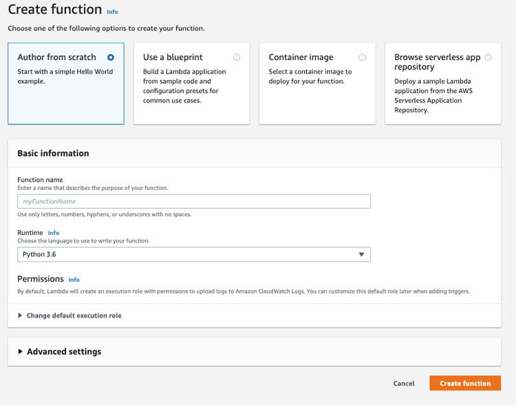
- Choose Create function.
- Select Author from scratch.
- For Function name, enter a name.
- For Runtime, choose Python 3.7.
- For Choose or create an execution role, choose Use an existing role.
- Choose service-role/AWSDeepLensLambdaRole.
- Choose Create function.
- On the function’s detail page, on the Actions menu, choose Upload a .zip file.
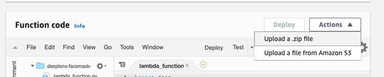
- Upload the inference Lambda file you downloaded earlier.
- Choose Save to save the code you entered.
- On the Actions menu, choose Publish new version.
Publishing the function makes it available on the AWS DeepLens console so that you can add it to your custom project.
- Enter a version number and choose Publish.
Understanding the inference function
This section walks you through some important parts of the inference function. First, you should pay attention to two specific files:
- labels.txt – Contains a mapping of the output from the neural network (integers) to human readable labels (string)
- lambda_function.py – Contains code for the function being called to generate predictions on every camera frame and send back results
In lambda_function.py, you first load and optimize the model. Compared to cloud virtual machines with a GPU, AWS DeepLens has less computing power. AWS DeepLens uses the Intel OpenVino model optimizer to optimize the model trained in SageMaker to run on its hardware. The following code optimizes your model to run locally:
client.publish(topic=iot_topic, payload='Optimizing model...')
ret, model_path = mo.optimize('deploy_ssd_resnet50_300', INPUT_W, INPUT_H)

# Load the model onto the GPU.
client.publish(topic=iot_topic, payload='Loading model...')
model = awscam.Model(model_path, {'GPU': 1})
Then you run the model frame-per-frame over the images from the camera. See the following code:
while True:
    # Get a frame from the video stream
    ret, frame = awscam.getLastFrame()
    if not ret:
        raise Exception('Failed to get frame from the stream')
    # Resize frame to the same size as the training set.
    frame_resize = cv2.resize(frame, (INPUT_H, INPUT_W))
    # Run the images through the inference engine and parse the results using
    # the parser API, note it is possible to get the output of doInference
    # and do the parsing manually, but since it is a ssd model,
    # a simple API is provided.
    parsed_inference_results = model.parseResult(model_type,
                                                 model.doInference(frame_resize))
Finally, you send the text prediction results back to the cloud. Viewing the text results in the cloud is a convenient way to make sure that the model is working correctly. Each AWS DeepLens device has a dedicated iot_topic automatically created to receive the inference results. See the following code:
# Send results to the cloud
client.publish(topic=iot_topic, payload=json.dumps(cloud_output))
Create a custom AWS DeepLens project
To create a new AWS DeepLens project, complete the following steps:
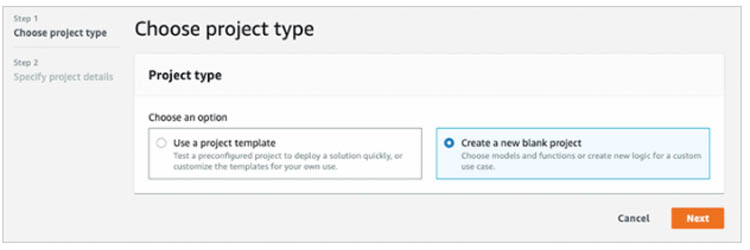
- On the AWS DeepLens console, on the Projects page, choose Create project.
- For Project type, select Create a new blank project.
- Choose Next.
- Name your project
yourname-pedestrian-detector-.
- Choose Add model.
- Select the model you just created.
- Choose Add function.
- Search for the Lambda function you created earlier by name.
- Choose Create project.
- On the Projects page, select the project you want to deploy.
- Chose Deploy to device.
- For Target device, choose your device.
- Choose Review.
- Review your settings and choose Deploy.
The deployment can take up to 10 minutes to complete, depending on the speed of the network your AWS DeepLens is connected to. When the deployment is complete, you should see a green banner on the page with the message, “Congratulations, your model is now running locally on AWS DeepLens!”
To see the text output, scroll down on the device details page to the Project output section. Follow the instructions in the section to copy the topic and go to the AWS IoT Core console to subscribe to the topic. You should see results as in the following screenshot.
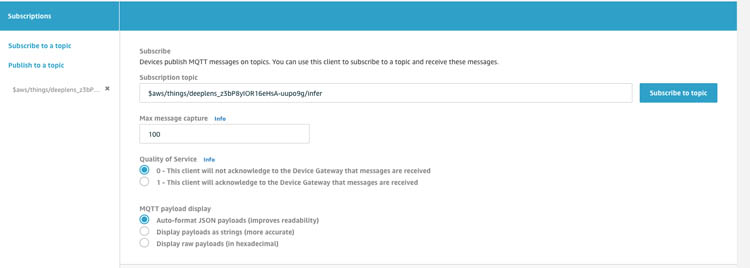
For step-by-step instructions on viewing the video stream or text output, see Viewing results from AWS DeepLens.
Real-world use cases
Now that you have predictions from your model running on AWS DeepLens, let’s convert those predictions into alerts and insights. Some most common uses for a project like this include:
- Understanding how many people on a given day entered a restricted zone so construction sites can identify spots that require more safety signs. This can be done by collecting the results and using them to create a dashboard using Amazon QuickSight. For more details about creating a dashboard using QuickSight, see Build a work-from-home posture tracker with AWS DeepLens and GluonCV.
- Collecting the output from AWS DeepLens and configuring a Raspberry Pi to sound an alert when someone is walking into a restricted zone. For more details about connecting an AWS DeepLens device to a Raspberry Pi device, see Building a trash sorter with AWS DeepLens.
Conclusion
In this post, you learned how to train an object detection model and deploy it to AWS DeepLens to detect people entering restricted zones. You can use this tutorial as a reference to train and deploy your own custom object detection projects on AWS DeepLens.
For a more detailed walkthrough of this tutorial and other tutorials, samples, and project ideas with AWS DeepLens, see AWS DeepLens Recipes.
About the Authors
 Yash Shah is a data scientist in the Amazon ML Solutions Lab, where he works on a range of machine learning use cases from healthcare to manufacturing and retail. He has a formal background in Human Factors and Statistics, and was previously part of the Amazon SCOT team designing products to guide 3P sellers with efficient inventory management.
 Phu Nguyen is a Product Manager for AWS Panorama. He builds products that give developers of any skill level an easy, hands-on introduction to machine learning.
Read More
 Tim Pavlick, PhD, is VP of Product at HawkEye 360. He is responsible for the conception, creation, and productization of all HawkEye space innovations. Mission Space is HawkEye 360’s flagship product, incorporating all the data and analytics from the HawkEye portfolio into one intuitive RF experience. Dr. Pavlick’s prior invention contributions include Myca, IBM’s AI Career Coach, Grit PTSD monitor for Veterans, IBM Defense Operations Platform, Smarter Planet Intelligent Operations Center, AI detection of dangerous hate speech on the internet, and the STORES electronic food ordering system for the US military. Dr. Pavlick received his PhD in Cognitive Psychology from the University of Maryland College Park.
 Ian Avilez is a Data Scientist with HawkEye 360. He works with customers to highlight the insights that can be gained by combining different datasets and looking at that data in various ways.
 Dan Ford is a Data Scientist at the Amazon ML Solution Lab, where he helps AWS National Security customers build state-of-the-art ML solutions.
 Gaurav Rele is a Data Scientist at the Amazon ML Solution Lab, where he works with AWS customers across different verticals to accelerate their use of machine learning and AWS Cloud services to solve their business challenges.


 Rizwan Gilani is a Software Development Engineer at Amazon SageMaker. His passion lies with making machine learning more interactive and accessible at scale. Before that, he worked on Amazon Alexa as part of the core team that launched Alexa Communications.
 Phi Nguyen is a solutions architect at AWS helping customers with their cloud journey with a special focus on data lake, analytics, semantics technologies and machine learning. In his spare time, you can find him biking to work, coaching his son’s soccer team or enjoying nature walk with his family.
 Arunprasath Shankar is an Artificial Intelligence and Machine Learning (AI/ML) Specialist Solutions Architect with AWS, helping global customers scale their AI solutions effectively and efficiently in the cloud. In his spare time, Arun enjoys watching sci-fi movies and listening to classical music.