Everything You Need To Know About Torchvision’s SSDlite Implementation

In the previous article, we’ve discussed how the SSD algorithm works, covered its implementation details and presented its training process. If you have not read the previous blog post, I encourage you to check it out before continuing.

In this part 2 of the series, we will focus on the mobile-friendly variant of SSD called SSDlite. Our plan is to first go through the main components of the algorithm highlighting the parts that differ from the original SSD, then discuss how the released model was trained and finally provide detailed benchmarks for all the new Object Detection models that we explored.

The SSDlite Network Architecture

The SSDlite is an adaptation of SSD which was first briefly introduced on the MobileNetV2 paper and later reused on the MobileNetV3 paper. Because the main focus of the two papers was to introduce novel CNN architectures, most of the implementation details of SSDlite were not clarified. Our code follows all the details presented on the two papers and where necessary fills the gaps from the official implementation.

As noted before, the SSD is a family of models because one can configure it with different backbones (such as VGG, MobileNetV3 etc) and different Heads (such as using regular convolutions, separable convolutions etc). Thus many of the SSD components remain the same in SSDlite. Below we discuss only those that are different

Classification and Regression Heads

Following the Section 6.2 of the MobileNetV2 paper, SSDlite replaces the regular convolutions used on the original Heads with separable convolutions. Consequently, our implementation introduces new heads that use 3×3 Depthwise convolutions and 1×1 projections. Since all other components of the SSD method remain the same, to create an SSDlite model our implementation initializes the SSDlite head and passes it directly to the SSD constructor.

Backbone Feature Extractor

Our implementation introduces a new class for building MobileNet feature extractors. Following the Section 6.3 of the MobileNetV3 paper, the backbone returns the output of the expansion layer of the Inverted Bottleneck block which has an output stride of 16 and the output of the layer just before the pooling which has an output stride of 32. Moreover, all extra blocks of the backbone are replaced with lightweight equivalents which use a 1×1 compression, a separable 3×3 convolution with stride 2 and a 1×1 expansion. Finally to ensure that the heads have enough prediction power even when small width multipliers are used, the minimum depth size of all convolutions is controlled by the min_depth hyperparameter.

The SSDlite320 MobileNetV3-Large model

This section discusses the configuration of the provided SSDlite pre-trained model along with the training processes followed to replicate the paper results as closely as possible.

Training process

All of the hyperparameters and scripts used to train the model on the COCO dataset can be found in our references folder. Here we discuss the most notable details of the training process.

Tuned Hyperparameters

Though the papers don’t provide any information on the hyperparameters used for training the models (such as regularization, learning rate and the batch size), the parameters listed in the configuration files on the official repo were good starting points and using cross validation we adjusted them to their optimal values. All the above gave us a significant boost over the baseline SSD configuration.

Data Augmentation

Key important difference of SSDlite comparing to SSD is that the backbone of the first has only a fraction of the weights of the latter. This is why in SSDlite, the Data Augmentation focuses more on making the model robust to objects of variable sizes than trying to avoid overfitting. Consequently, SSDlite uses only a subset of the SSD transformations and this way it avoids the over-regularization of the model.

LR Scheme

Due to the reliance on Data Augmentation to make the model robust to small and medium sized objects, we found that it is particularly beneficial for the training recipe to use large number of epochs. More specifically by using roughly 3x more epochs than SSD we are able to increase our precision by 4.2mAP points and by using a 6x multiplier we improve by 4.9mAP. Increasing further the epochs seems to yield diminishing returns and makes the training too slow and impractical, nevertheless based on the model configuration it seems that the authors of the paper used an equivalent 16x multiplier.

Weight Initialization & Input Scaling & ReLU6

A set of final optimizations that brought our implementation very close to the official one and helped us bridge the accuracy gap was training the backbone from scratch instead of initializing from ImageNet, adapting our weight initialization scheme, changing our Input Scaling and replacing all standard ReLUs added on the SSDlite heads with ReLU6. Note that since we trained the model from random weights, we additionally applied the speed optimization described on the paper of using a reduced tail on the backbone.

Implementation Differences

Comparing the above implementation with the one on the official repo, we’ve identified a few differences. Most of them are minor and they are related to how we initialize the weights (for example Normal initialization vs Truncated Normal), how we parameterize the LR Scheduling (for example smaller vs larger warmup rate, shorter vs longer training) etc. The biggest known difference lies in the way we compute the Classification loss. More specifically the implementation of SSDlite with MobileNetV3 backbone on the official repo doesn’t use the SSD’s Multibox loss but instead uses RetinaNet’s focal loss. This is a rather significant deviation from the paper and since TorchVision already offers a full implementation of RetinaNet, we decided to implement SSDlite using the normal Multi-box SSD loss.

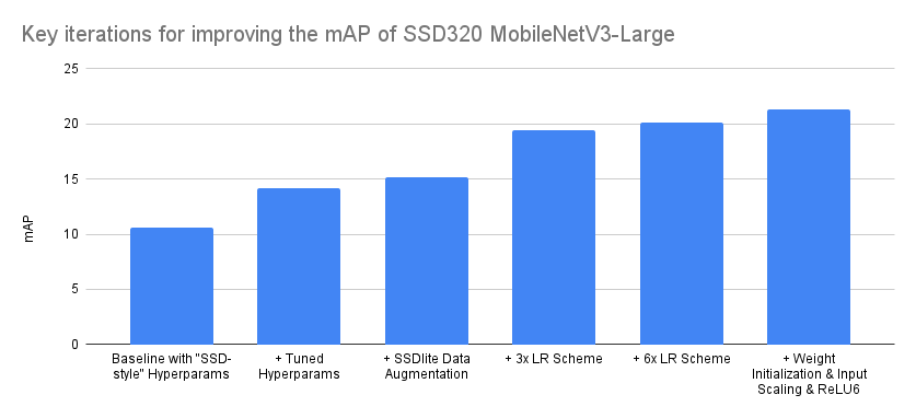
Break down of key accuracy improvements

As discussed in previous articles, reproducing research papers and porting them to code is not a journey of monotonically increasing accuracies, especially in cases where the full training and implementation details are not known. Typically the process involves lots of backtracking as one needs to identify those implementation details and parameters that have significant impact on the accuracy from those that don’t. Below we try to visualize the most important iterations that improved our accuracy from the baseline:

Iteration mAP
Baseline with “SSD-style” Hyperparams 10.6
+ Tuned Hyperparams 14.2
+ SSDlite Data Augmentation 15.2
+ 3x LR Scheme 19.4
+ 6x LR Scheme 20.1
+ Weight Initialization & Input Scaling & ReLU6 21.3

The order of optimizations presented above is accurate, though a bit idealized in some cases. For example, though different schedulers were tested during the Hyperparameter tuning phase, none of them provided significant improvements and thus we maintained the MultiStepLR which was used in the baseline. Nevertheless while later experimenting with different LR Schemes, we found it beneficial to switch to CosineAnnealingLR, as it required less configuration. Consequently, we believe that the main takeaway from the above summary should be that even by starting with a correct implementation and a set of optimal hyperparams from a model of the same family, there is always accuracy points to be found by optimizing the training recipe and tuning the implementation. Admittedly the above is a rather extreme case where the accuracy doubled, but still in many cases there is a large number of optimizations that can help us push the accuracy significantly.

Benchmarks

Here is how to initialize the two pre-trained models:

ssdlite = torchvision.models.detection.ssdlite320_mobilenet_v3_large(pretrained=True)
ssd = torchvision.models.detection.ssd300_vgg16(pretrained=True)

Below are the benchmarks between the new and selected previous detection models:

Model mAP Inference on CPU (sec) # Params (M)
SSDlite320 MobileNetV3-Large 21.3 0.0911 3.44
SSD300 VGG16 25.1 0.8303 35.64
SSD512 VGG16 (not released) 28.8 2.2494 37.08
SSD512 ResNet50 (not released) 30.2 1.1137 42.70
Faster R-CNN MobileNetV3-Large 320 FPN (Low-Res) 22.8 0.1679 19.39
Faster R-CNN MobileNetV3-Large FPN (High-Res) 32.8 0.8409 19.39

As we can see, the SSDlite320 MobileNetV3-Large model is by far the fastest and smallest model and thus it’s an excellent candidate for real-world mobile applications. Though its accuracy is lower than the pre-trained low-resolution Faster R-CNN equivalent, the SSDlite framework is adaptable and one can boost its accuracy by introducing heavier heads with more convolutions.

On the other hand, the SSD300 VGG16 model is rather slow and less accurate. This is mainly because of its VGG16 backbone. Though extremely important and influential, the VGG architecture is nowadays quite outdated. Thus though the specific model has historical and research value and hence it’s included in TorchVision, we recommend to users who want high-resolution detectors for real world applications to either combine SSD with alternative backbones (see this example on how to create one) or use one of the Faster R-CNN pre-trained models.

We hope you enjoyed the 2nd and final part of the SSD series. We are looking forward to your feedback.

Read More

Achieving Precision in Quantum Material Simulations

Posted by Charles Neill and Zhang Jiang, Senior Research Scientists, Google Quantum AI

In fall of 2019, we demonstrated that the Sycamore quantum processor could outperform the most powerful classical computers when applied to a tailor-made problem. The next challenge is to extend this result to solve practical problems in materials science, chemistry and physics. But going beyond the capabilities of classical computers for these problems is challenging and will require new insights to achieve state-of-the-art accuracy. Generally, the difficulty in performing quantum simulations of such physical problems is rooted in the wave nature of quantum particles, where deviations in the initial setup, interference from the environment, or small errors in the calculations can lead to large deviations in the computational result.

In two upcoming publications, we outline a blueprint for achieving record levels of precision for the task of simulating quantum materials. In the first work, we consider one-dimensional systems, like thin wires, and demonstrate how to accurately compute electronic properties, such as current and conductance. In the second work, we show how to map the Fermi-Hubbard model, which describes interacting electrons, to a quantum processor in order to simulate important physical properties. These works take a significant step towards realizing our long-term goal of simulating more complex systems with practical applications, like batteries and pharmaceuticals.

A bottom view of one of the quantum dilution refrigerators during maintenance. During the operation, the microwave wires that are floating in this image are connected to the quantum processor, e.g., the Sycamore chip, bringing the temperature of the lowest stage to a few tens of milli-degrees above absolute zero temperature.

Computing Electronic Properties of Quantum Materials
In “Accurately computing electronic properties of a quantum ring”, to be published in Nature, we show how to reconstruct key electronic properties of quantum materials. The focus of this work is on one-dimensional conductors, which we simulate by forming a loop out of 18 qubits on the Sycamore processor in order to mimic a very narrow wire. We illustrate the underlying physics through a series of simple text-book experiments, starting with a computation of the “band-structure” of this wire, which describes the relationship between the energy and momentum of electrons in the metal. Understanding such structure is a key step in computing electronic properties such as current and conductance. Despite being an 18-qubit algorithm consisting of over 1,400 logical operations, a significant computational task for near-term devices, we are able to achieve a total error as low as 1%.

The key insight enabling this level of accuracy stems from robust properties of the Fourier transform. The quantum signal that we measure oscillates in time with a small number of frequencies. Taking a Fourier transform of this signal reveals peaks at the oscillation frequencies (in this case, the energy of electrons in the wire). While experimental imperfections affect the height of the observed peaks (corresponding to the strength of the oscillation), the center frequencies are robust to these errors. On the other hand, the center frequencies are especially sensitive to the physical properties of the wire that we hope to study (e.g., revealing small disorders in the local electric field felt by the electrons). The essence of our work is that studying quantum signals in the Fourier domain enables robust protection against experimental errors while providing a sensitive probe of the underlying quantum system.

(Left) Schematic of the 54-qubit quantum processor, Sycamore. Qubits are shown as gray crosses and tunable couplers as blue squares. Eighteen of the qubits are isolated to form a ring. (Middle) Fourier transform of the measured quantum signal. Peaks in the Fourier spectrum correspond to the energy of electrons in the ring. Each peak can be associated with a traveling wave that has fixed momentum. (Right) The center frequency of each peak (corresponding to the energy of electrons in the wire) is plotted versus the peak index (corresponding to the momentum). The measured relationship between energy and momentum is referred to as the ‘band structure’ of the quantum wire and provides valuable information about electronic properties of the material, such as current and conductance.

Quantum Simulation of the Fermi-Hubbard Model
In “Observation of separated dynamics of charge and spin in the Fermi-Hubbard model”, we focus on the dynamics of interacting electrons. Interactions between particles give rise to novel phenomena such as high temperature superconductivity and spin-charge separation. The simplest model that captures this behavior is known as the Fermi-Hubbard model. In materials such as metals, the atomic nuclei form a crystalline lattice and electrons hop from lattice site to lattice site carrying electrical current. In order to accurately model these systems, it is necessary to include the repulsion that electrons feel when getting close to one another. The Fermi-Hubbard model captures this physics with two simple parameters that describe the hopping rate (J) and the repulsion strength (U).

We realize the dynamics of this model by mapping the two physical parameters to logical operations on the qubits of the processor. Using these operations, we simulate a state of the electrons where both the electron charge and spin densities are peaked near the center of the qubit array. As the system evolves, the charge and spin densities spread at different rates due to the strong correlations between electrons. Our results provide an intuitive picture of interacting electrons and serve as a benchmark for simulating quantum materials with superconducting qubits.

(Left top) Illustration of the one-dimensional Fermi-Hubbard model in a periodic potential. Electrons are shown in blue, with their spin indicated by the connected arrow. J, the distance between troughs in the electric potential field, reflects the “hopping” rate, i.e., the rate at which electrons transition from one trough in the potential to another, and U, the amplitude, represents the strength of repulsion between electrons. (Left bottom) The simulation of the model on a qubit ladder, where each qubit (square) represents a fermionic state with spin-up or spin-down (arrows). (Right) Time evolution of the model reveals separated spreading rates of charge and spin. Points and solid lines represent experimental and numerical exact results, respectively. At t = 0, the charge and spin densities are peaked at the middle sites. At later times, the charge density spreads and reaches the boundaries faster than the spin density.

Conclusion
Quantum processors hold the promise to solve computationally hard tasks beyond the capability of classical approaches. However, in order for these engineered platforms to be considered as serious contenders, they must offer computational accuracy beyond the current state-of-the-art classical methods. In our first experiment, we demonstrate an unprecedented level of accuracy in simulating simple materials, and in our second experiment, we show how to embed realistic models of interacting electrons into a quantum processor. It is our hope that these experimental results help progress the goal of moving beyond the classical computing horizon.

Read More

Meet TensorFlow community leads around the world

Posted by Joana Carrasqueira and Lynette Gaddi, Program Managers at Google

The TensorFlow community keeps growing every day, and includes many thousands of developers, educators, and researchers around the world. If you’d like to get involved with the community, there are many different organizations you can check out.

These include Special Interest Groups (SIGs), TensorFlow User Groups (TFUGs), and Google Developer Groups (GDGs). There are also many Google Developer Experts (GDEs) you can get in touch with. They’re knowledgeable about ML and help others in their community, and are a great point of contact to find future local events.

We spend a lot of time working with community leads, and in this article, we’d like to share some of their stories with you. We had the wonderful opportunity to interview several leads from different areas – including a SIG Lead, a Machine Learning GDE, and two TensorFlow User Group organizers, so you can learn about their background, how they got involved in the community, and how you can too.

TensorFlow branded banner with orange elements

Karl Lessard

TensorFlow SIG Lead for JVM

Montreal, Canada

Image of Karl Lessard

Karl has been working in software engineering and consulting for more than 20 years in various fields, including computer graphics and communications. He is now working full-time at Expedia in Montreal, focusing on delivering solutions for complex linguistic and localization challenges.

What does being a community leader mean to you?

What really matters is that all members of the group enjoy contributing to the project, and making it as fulfilling as possible for them. Because that’s what open-source is to me: a playground for grownups building something useful to the world! Being a community leader comes with a bunch of technical responsibilities, too, but for me that’s the most important thing.

How did you get involved in the TF community?

I started designing a few proposals to enhance the TensorFlow Java client, which at that time was offering minimal support for running model inference on Android devices. My proposed changes were welcomed by Google (special thanks to Asim Shankar), and I’ve submitted multiple pull requests over a couple years since then.

There was increasing general interest in supporting TensorFlow on the JVM following that, and I met the engineering team (and many others from the community) at a TensorFlow Dev summit in 2019 to suggest the idea of starting a group focusing on this topic. That’s how SIG JVM was born.

How do you contribute technically as a SIG Lead?

I still contribute to the design and the code of the project (like in the beginning), but I also review most of the pull requests, plan video calls, and make sure proposed changes are done with respect to the global vision of the project shared by other members, and they are being discussed properly and broadly.

Do you have any advice on how to get involved in the community?

If you can make it to the TensorFlow Dev/Contributor Summit, do it. That’s definitely a good place to meet people sharing the same interests as you. Also, you can get involved in the various discussions related to the topics of your interests. SIGs forums are a good place to start, and you can also get in touch with others on the new TensorFlow Forum. Finally, don’t be shy to make change proposals and/or to submit a few pull requests!

Ruqiya Bin Safi

Google Cloud GDE

Saudi Arabia

image of Ruqiya Bin Safi

Ruqiya Bin Safi is a Software Engineer that is interested in Artificial Intelligence, Machine Learning and Deep Learning as well as Data Science. Ruqiya started learning Machine Learning many years ago. She seeks to spread knowledge about Machine Learning and new technologies.

What does being a community leader mean to you?

It means a responsibility I take on, a goal I’ve accomplished, and a dream I fulfill. It means that I contribute to the development of my community and helping others. To be a community leader means sharing useful knowledge so that everyone can benefit. Leadership is also a give and take: the community gives to me, and I give back to the community. It’s a cooperation. We share similar goals and interests, and vision and mission. And we seek to employ what we’ve learned to develop tools that make the world a better place.

How did you get involved in the TF community?

I’ve always loved learning new technologies and using them to solve problems. I started as a software engineer, and found machine learning increasingly interesting as I studied it, and eventually made it a focus. I got involved with the TF community through a Women Techmakers (WTM) event. I then joined a local WTM community to help others learn about ML, and later applied and was accepted into the GDE program.

How do you contribute as a ML GDE?

I love giving talks, and most of my contributions were as speaker and technical trainer through various tech talks, panel discussions, and workshops. My goal is to help and motivate people to learn more about ML. I also run a deep learning monthly workshop that aims to help participants gain foundational knowledge of common deep learning techniques as well as practical experience in building neural networks with TensorFlow. I also really enjoy mentoring for Google for Startups Accelerator MENA program as well as some hackathons, and I write articles from time to time about machine learning and TensorFlow.

Do you have any advice on how to get involved in the community?

One of the best ways is to try to learn something new, and then share what you have learned with your community through blogging or a local meetup. Love what you do, and as much as you can, find work that you enjoy – and trust in yourself as you become more active and involved.

Armel Yara

TensorFlow User Group, Organizer

Abidja, West Africa

Photo of Armel Yara

Armel is a developer and TensorFlow community leader in Francophone Africa, where he organizes and hosts developer events in multiple languages (including large events like TensorFlow Everywhere SSA), and manages machine learning projects for local business

What does being a community leader mean to you?

Being a community leader means for me sharing experiences, being available for others, and listening to their needs and expectations.

How did you get involved in the TF community?

I get involved in the TF community by sharing the latest news about the TF community on my blog and working on open source projects.

How do you contribute as a TFUG lead?

I organize events and give technical sessions at universities and online.

Do you have any advice on how to get involved in the community?

My advice to become more active and get more involved in the community is to look over the membership expectations, share projects that you have built, and use them to motivate others. Lead by example, let others know how much you enjoy what you do and showcase your work.

Nijat Zeynalov

TensorFlow User Group, Organizer

Azerbaijan

photo of Nijat Zeynalov

Nijat is a Certified TensorFlow Developer and a first year master student at University of Tartu. He’s passionate about data science and machine learning, and organizing events to help others.

What does being a community leader mean to you?

I learned about leadership by running a local community where we aimed to provide free support to anyone interested in coding. In my mind, being a community leader means to help inspire others, and also to foster a community of respect that enables and encourages contributions of others. I strongly believe that leadership can be learned with practice.

How did you get involved in the TF community?

While I was preparing for the TensorFlow Developer certificate, I found a user groups page and I thought – why not set up a local user group for our country. I understood the responsibility of being a community leader, and I contacted a few TensorFlow User Group organizers to learn more about it. Their positive feedback about the overall impression made my decision even easier and motivated me to get started, and it’s been a great experience ever since.

How do you contribute as a community organizer?

We regularly discuss the latest TensorFlow updates in the user group, and we organise “Paper Reading Meetings” where we read and discuss one deep learning paper as a group. This has been a really great way for people to share their knowledge and ask questions. Additionally, in March, as a “TensorFlow User Group – Azerbaijan”, we held the 5-hour long “TensorFlow Everywhere – 2021” event which was the country’s largest machine learning event to date.

It was a pleasure to speak with Karl, Ruqiya, Armel and Nijat (thank you again for your time and contributions!) We hope their stories inspire you to get involved, and take on a leadership role in your local community in the future. If you’d like, you can start a conversation on the TensorFlow Forum and share how you got involved in the TensorFlow Community, and meet others. And check out the top of this post for more links to user and special interest groups.

Read More

A Dataset for Studying Gender Bias in Translation

Posted by Romina Stella, Product Manager, Google Translate

Advances on neural machine translation (NMT) have enabled more natural and fluid translations, but they still can reflect the societal biases and stereotypes of the data on which they’re trained. As such, it is an ongoing goal at Google to develop innovative techniques to reduce gender bias in machine translation, in alignment with our AI Principles.

One research area has been using context from surrounding sentences or passages to improve gender accuracy. This is a challenge because traditional NMT methods translate sentences individually, but gendered information is not always explicitly stated in each individual sentence. For example, in the following passage in Spanish (a language where subjects aren’t always explicitly mentioned), the first sentence refers explicitly to Marie Curie as the subject, but the second one doesn’t explicitly mention the subject. In isolation, this second sentence could refer to a person of any gender. When translating to English, however, a pronoun needs to be picked, and the information needed for an accurate translation is in the first sentence.

Spanish Text Translation to English
Marie Curie nació en Varsovia. Fue la primera persona en recibir dos premios Nobel en distintas especialidades. Marie Curie was born in Warsaw. She was the first person to receive two Nobel Prizes in different specialties.

Advancing translation techniques beyond single sentences requires new metrics for measuring progress and new datasets with the most common context-related errors. Adding to this challenge is the fact that translation errors related to gender (such as picking the correct pronoun or having gender agreement) are particularly sensitive, because they may directly refer to people and how they self identify.

To help facilitate progress against the common challenges on contextual translation (e.g., pronoun drop, gender agreement and accurate possessives), we are releasing the Translated Wikipedia Biographies dataset, which can be used to evaluate the gender bias of translation models. Our intent with this release is to support long-term improvements on ML systems focused on pronouns and gender in translation by providing a benchmark in which translations’ accuracy can be measured pre- and post-model changes.

A Source of Common Translation Errors
Because they are well-written, geographically diverse, contain multiple sentences, and refer to subjects in the third person (and so contain plenty of pronouns), Wikipedia biographies offer a high potential for common translation errors associated with gender. These often occur when articles refer to a person explicitly in early sentences of a paragraph, but there is no explicit mention of the person in later sentences. Some examples:

Translation Error     Text     Translation
Pro-drop in Spanish → English     Marie Curie nació en Varsovia. Recibió el Premio Nobel en 1903 y en 1911.     Marie Curie was born in Warsaw. He received the Nobel Prize in 1903 and in 1911.
Neutral possessives in Spanish → English     Marie Curie nació en Varsovia. Su carrera profesional fue desarrollada en Francia.     Marie Curie was born in Warsaw. His professional career was developed in France.
Gender agreement in English → German     Marie Curie was born in Warsaw. The distinguished scientist received the Nobel Prize in 1903 and in 1911.     Marie Curie wurde in Varsovia geboren. Der angesehene Wissenschaftler erhielt 1903 und 1911 den Nobelpreis.
Gender agreement in English → Spanish     Marie Curie was born in Warsaw. The distinguished scientist received the Nobel Prize in 1903 and in 1911.     Marie Curie nació en Varsovia. El distinguido científico recibió el Premio Nobel en 1903 y en 1911.

Building the Dataset
The Translated Wikipedia Biographies dataset has been designed to analyze common gender errors in machine translation, such as those illustrated above. Each instance of the dataset represents a person (identified in the biographies as feminine or masculine), a rock band or a sports team (considered genderless). Each instance is represented by a long text translation of 8 to 15 connected sentences referring to that central subject (the person, rock band, or sports team). Articles are written in native English and have been professionally translated to Spanish and German. For Spanish, translations were optimized for pronoun-drop, so the same set could be used to analyze pro-drop (Spanish → English) and gender agreement (English → Spanish).

The dataset was built by selecting a group of instances that has equal representation across geographies and genders. To do this, we extracted biographies from Wikipedia according to occupation, profession, job and/or activity. To ensure an unbiased selection of occupations, we chose nine occupations that represented a range of stereotypical gender associations (either feminine, masculine, or neither) based on Wikipedia statistics. Then, to mitigate any geography-based bias, we divided all these instances based on geographical diversity. For each occupation category, we looked to have one candidate per region (using regions from census.gov as a proxy of geographical diversity). When an instance was associated with a region, we checked that the selected person had a relevant relationship with a country that belongs to a designated region (nationality, place of birth, lived for a big portion of their life, etc.). By using this criteria, the dataset contains entries about individuals from more than 90 countries and all regions of the world.

Although gender is non-binary, we focused on having equal representation of “feminine” and “masculine” entities. It’s worth mentioning that because the entities are represented as such on Wikipedia, the set doesn’t include individuals that identify as non-binary, as, unfortunately, there are not enough instances currently represented in Wikipedia to accurately reflect the non-binary community. To label each instance as “feminine” or “masculine” we relied on the biographical information from Wikipedia, which contained gender-specific references to the person (she, he, woman, son, father, etc.).

After applying all these filters, we randomly selected an instance for each occupation-region-gender triplet. For each occupation, there are two biographies (one masculine and one feminine), for each of the seven geographic regions.

Finally, we added 12 instances with no gender. We picked rock bands and sports teams because they are usually referred to by non-gendered third person pronouns (such as “it” or singular “they”). The purpose of including these instances is to study over triggering, i.e., when models learn that they are rewarded for producing gender-specific pronouns, leading them to produce these pronouns in cases where they shouldn’t.

Results and Applications
This dataset enables a new method of evaluation for gender bias reduction in machine translations (introduced in a previous post). Because each instance refers to a subject with a known gender, we can compute the accuracy of the gender-specific translations that refer to this subject. This computation is easier when translating into English (cases of languages with pro-drop or neutral pronouns) since computation is mainly based on gender-specific pronouns in English. In these cases, the gender datasets have resulted in a 67% reduction in errors on context-aware models vs. previous models. As mentioned before, the neutral entities have allowed us to discover cases of over triggering like the usage of feminine or masculine pronouns to refer to genderless entities. This new dataset also enables new research directions into the performance of different models across types of occupations or geographic regions.

As an example, the dataset allowed us to discover the following improvements in an excerpt of the translated biography of Marie Curie from Spanish.

Translation result with the previous NMT model.
Translation result with the new contextual model.

Conclusion
This Translated Wikipedia Biographies dataset is the result of our own studies and work on identifying biases associated with gender and machine translation. This set focuses on a specific problem related to gender bias and doesn’t aim to cover the whole problem. It’s worth mentioning that by releasing this dataset, we don’t aim to be prescriptive in determining what’s the optimal approach to address gender bias. This contribution aims to foster progress on this challenge across the global research community.

Acknowledgements
The datasets were built with help from Anja Austermann, Melvin Johnson, Michelle Linch, Mengmeng Niu, Mahima Pushkarna, Apu Shah, Romina Stella, and Kellie Webster.

Read More

Improving Genomic Discovery with Machine Learning

Posted by Andrew Carroll, Product Manager and Cory McLean, Software Engineer, Google Health

Each person’s genome, which collectively encodes the biochemical machinery they are born with, is composed of over 3 billion letters of DNA. However, only a small subset of the genome (~4-5 million positions) varies between two people. Nonetheless, each person’s unique genome interacts with the environment they experience to determine the majority of their health outcomes. A key method of understanding the relationship between genetic variants and traits is a genome-wide association study (GWAS), in which each genetic variant present in a cohort is individually examined for correlation with the trait of interest. GWAS results can be used to identify and prioritize potential therapeutic targets by identifying genes that are strongly associated with a disease of interest, and can also be used to build a polygenic risk score (PRS) to predict disease predisposition based on the combined influence of variants present in an individual. However, while accurate measurement of traits in an individual (called phenotyping) is essential to GWAS, it often requires painstaking expert curation and/or subjective judgment calls.

In “Large-scale machine learning-based phenotyping significantly improves genomic discovery for optic nerve head morphology”, we demonstrate how using machine learning (ML) models to classify medical imaging data can be used to improve GWAS. We describe how models can be trained for phenotypes to generate trait predictions and how these predictions are used to identify novel genetic associations. We then show that the novel associations discovered improve PRS accuracy and, using glaucoma as an example, that the improvements for anatomical eye traits relate to human disease. We have released the model training code and detailed documentation for its use on our Genomics Research GitHub repository.

Identifying genetic variants associated with eye anatomical traits
Previous work has demonstrated that ML models can identify eye diseases, skin diseases, and abnormal mammogram results with accuracy approaching or exceeding state-of-the-art methods by domain experts. Because identifying disease is a subset of phenotyping, we reasoned that ML models could be broadly used to improve the speed and quality of phenotyping for GWAS.

To test this, we chose a model that uses a fundus image of the eye to accurately predict whether a patient should be referred for assessment for glaucoma. This model uses the fundus images to predict the diameters of the optic disc (the region where the optic nerve connects to the retina) and the optic cup (a whitish region in the center of the optic disc). The ratio of the diameters of these two anatomical features (called the vertical cup-to-disc ratio, or VCDR) correlates strongly with glaucoma risk.

A representative retinal fundus image showing the vertical cup-to-disc ratio, which is an important diagnostic measurement for glaucoma.

We applied this model to predict VCDR in all fundus images from individuals in the UK Biobank, which is the world’s largest dataset available to researchers worldwide for health-related research in the public interest, containing extensive phenotyping and genetic data for ~500,000 pseudonymized (the UK Biobank’s standard for de-identification) individuals. We then performed GWAS in this dataset to identify genetic variants that are associated with the model-based predictions of VCDR.

Applying a VCDR prediction model trained on clinical data to generate predicted values for VCDR to enable discovery of genetic associations for the VCDR trait.

The ML-based GWAS identified 156 distinct genomic regions associated with VCDR. We compared these results to a VCDR GWAS conducted by another group on the same UK Biobank data, Craig et al. 2020, where experts had painstakingly labeled all images for VCDR. The ML-based GWAS replicates 62 of the 65 associations found in Craig et al., which indicates that the model accurately predicts VCDR in the UK Biobank images. Additionally, the ML-based GWAS discovered 93 novel associations.

Number of statistically significant GWAS associations discovered by exhaustive expert labeling approach (Craig et al., left), and by our ML-based approach (right), with shared associations in the middle.

The ML-based GWAS improves polygenic model predictions
To validate that the novel associations discovered in the ML-based GWAS are biologically relevant, we developed independent PRSes using the Craig et al. and ML-based GWAS results, and tested their ability to predict human-expert-labeled VCDR in a subset of UK Biobank as well as a fully independent cohort (EPIC-Norfolk). The PRS developed from the ML-based GWAS showed greater predictive ability than the PRS built from the expert labeling approach in both datasets, providing strong evidence that the novel associations discovered by the ML-based method influence VCDR biology, and suggesting that the improved phenotyping accuracy (i.e., more accurate VCDR measurement) of the model translates into a more powerful GWAS.

The correlation between a polygenic risk score (PRS) for VCDR generated from the ML-based approach and the exhaustive expert labeling approach (Craig et al.). In these plots, higher values on the y-axis indicate a greater correlation and therefore greater prediction from only the genetic data. [* — p ≤ 0.05; *** — p ≤ 0.001]

As a second validation, because we know that VCDR is strongly correlated with glaucoma, we also investigated whether the ML-based PRS was correlated with individuals who had either self-reported that they had glaucoma or had medical procedure codes suggestive of glaucoma or glaucoma treatment. We found that the PRS for VCDR determined using our model predictions were also predictive of the probability that an individual had indications of glaucoma. Individuals with a PRS 2.5 or more standard deviations higher than the mean were more than 3 times as likely to have glaucoma in this cohort. We also observed that the VCDR PRS from ML-based phenotypes was more predictive of glaucoma than the VCDR PRS produced from the extensive manual phenotyping.

The odds ratio of glaucoma (self-report or ICD code) stratified by the PRS for VCDR determined using the ML-based phenotypes (in standard deviations from the mean). In this plot, the y-axis shows the probability that the individual has glaucoma relative to the baseline rate (represented by the dashed line). The x-axis shows standard deviations from the mean for the PRS. Data are visualized as a standard box plot, which illustrates values for the mean (the orange line), first and third quartiles, and minimum and maximum.

Conclusion
We have shown that ML models can be used to quickly phenotype large cohorts for GWAS, and that these models can increase statistical power in such studies. Although these examples were shown for eye traits predicted from retinal imaging, we look forward to exploring how this concept could generally apply to other diseases and data types.

Acknowledgments
We would like to especially thank co-author Dr. Anthony Khawaja of Moorfields Eye Hospital for contributing his extensive medical expertise. We also recognize the efforts of Professor Jamie Craig and colleagues for their exhaustive labeling of UK Biobank images, which allowed us to make comparisons with our method. Several authors of that work, as well as Professor Stuart MacGregor and collaborators in Australia and at Max Kelsen have independently replicated these findings, and we value these scientific contributions as well. Last, this work summarizes the work of the following Google contributors, who we would like to thank: Babak Alipanahi, Farhad Hormozdiari, Babak Behsaz, Justin Cosentino, Zachary R. McCaw, Emanuel Schorsch, D. Sculley, Elizabeth H. Dorfman, Sonia Phene, Naama Hammel, Andrew Carroll, and Cory Y. McLean

Read More

The torch.linalg module: Accelerated Linear Algebra with Autograd in PyTorch

Linear algebra is essential to deep learning and scientific computing, and it’s always been a core part of PyTorch. PyTorch 1.9 extends PyTorch’s support for linear algebra operations with the torch.linalg module. This module, documented here, has 26 operators, including faster and easier to use versions of older PyTorch operators, every function from NumPy’s linear algebra module extended with accelerator and autograd support, and a few operators that are completely new. This makes the torch.linalg immediately familiar to NumPy users and an exciting update to PyTorch’s linear algebra support.

NumPy-like linear algebra in PyTorch

If you’re familiar with NumPy’s linear algebra module then it’ll be easy to start using torch.linalg. In most cases it’s a drop-in replacement. Let’s looking at drawing samples from a multivariate normal distribution using the Cholesky decomposition as a motivating example to demonstrate this:

import numpy as np

# Creates inputs
np.random.seed(0)
mu_np = np.random.rand(4)
L = np.random.rand(4, 4)
# Covariance matrix sigma is positive-definite
sigma_np = L @ L.T + np.eye(4)
normal_noise_np = np.random.standard_normal(mu_np.size)

def multivariate_normal_sample_np(mu, sigma, normal_noise):
    return mu + np.linalg.cholesky(sigma) @ normal_noise

print("Random sample: ", 
      multivariate_normal_sample_np(mu_np, sigma_np, normal_noise_np))
: Random sample: [2.9502426 1.78518077 1.83168697 0.90798228]

Now let’s see the same sampler implemented in PyTorch:

import torch

def multivariate_normal_sample_torch(mu, sigma, normal_noise):
    return mu + torch.linalg.cholesky(sigma) @ normal_noise

The two functions are identical, and we can validate their behavior by calling the function with the same arguments wrapped as PyTorch tensors:

# NumPy arrays are wrapped as tensors and share their memory
mu_torch = torch.from_numpy(mu_np)
sigma_torch = torch.from_numpy(sigma_np)
normal_noise_torch = torch.from_numpy(normal_noise_np)

multivariate_normal_sample_torch(mu_torch, sigma_torch, normal_noise_torch)
: tensor([2.9502, 1.7852, 1.8317, 0.9080], dtype=torch.float64)

The only difference is in how PyTorch prints tensors by default.

The Cholesky decomposition can also help us quickly compute the probability density function of the non-degenerate multivariate normal distribution. One of the expensive terms in that computation is the square root of the determinant of the covariance matrix. Using properties of the determinant and the Cholesky decomposition we can calculate the same result faster than the naive computation, however. Here’s the NumPy program that demonstrates this:

sqrt_sigma_det_np = np.sqrt(np.linalg.det(sigma_np))
sqrt_L_det_np = np.prod(np.diag(np.linalg.cholesky(sigma_np)))

print("|sigma|^0.5 = ", sqrt_sigma_det_np)
: |sigma|^0.5 = 4.237127491242027
 
print("|L| = ", sqrt_L_det_np)
: |L| = 4.237127491242028

And here’s the same validation in PyTorch:

sqrt_sigma_det_torch = torch.sqrt(torch.linalg.det(sigma_torch))
sqrt_L_det_torch = torch.prod(torch.diag(torch.linalg.cholesky(sigma_torch)))

print("|sigma|^0.5 = ", sqrt_sigma_det_torch)
: |sigma|^0.5 = tensor(4.2371, dtype=torch.float64) 

print("|L| = ", sqrt_L_det_torch)
: |L| = tensor(4.2371, dtype=torch.float64)

We can measure the difference in run time using PyTorch’s built-in benchmark utility:

import torch.utils.benchmark as benchmark

t0 = benchmark.Timer(
    stmt='torch.sqrt(torch.linalg.det(sigma))',
    globals={'sigma': sigma_torch})

t1 = benchmark.Timer(
    stmt='torch.prod(torch.diag(torch.linalg.cholesky(sigma)))',
    globals={'sigma': sigma_torch})

print(t0.timeit(100))
: torch.sqrt(torch.linalg.det(sigma))
  80.80 us
  1 measurement, 100 runs , 1 thread


print(t1.timeit(100))
: torch.prod(torch.diag(torch.linalg.cholesky(sigma)))
  11.56 us
  1 measurement, 100 runs , 1 thread

Demonstrating that the approach using the Cholesky decomposition can be significantly faster. Behind the scenes, PyTorch’s linear algebra module uses OpenBLAS or MKL implementations of the LAPACK standard to maximize its CPU performance.

Autograd Support

PyTorch’s linear algebra module doesn’t just implement the same functions as NumPy’s linear algebra module (and a few more), it also extends them with autograd and CUDA support.

Let’s look at a very simple program that just computes an inverse and the gradient of that operation to show how autograd works:

t = torch.tensor(((1, 2), (3, 4)), dtype=torch.float32, requires_grad=True)

inv = torch.linalg.inv(t)
inv.backward(torch.ones_like(inv))

print(t.grad)
: tensor([[-0.5000, 0.5000],
          [ 0.5000, -0.5000]])

We can mimic the same computation in NumPy by defining the autograd formula ourselves:

a = np.array(((1, 2), (3, 4)), dtype=np.float32)

inv_np = np.linalg.inv(a)

def inv_backward(result, grad):
    return -(result.transpose(-2, -1) @ (grad @ result.transpose(-2, -1)))
grad_np = inv_backward(inv_np, np.ones_like(inv_np))

print(grad_np)
: [[-0.5 0.5]
   [ 0.5 -0.5]]

Of course, as programs become more complicated it’s convenient to have builtin autograd support, and PyTorch’s linear algebra module supports both real and complex autograd.

CUDA Support

Support for autograd and accelerators, like CUDA devices, is a core part of PyTorch. The torch.linalg module was developed with NVIDIA’s PyTorch and cuSOLVER teams, who helped optimize its performance on CUDA devices with the cuSOLVER, cuBLAS, and MAGMA libraries. These improvements make PyTorch’s CUDA linear algebra operations faster than ever. For example, let’s look at the performance of PyTorch 1.9’s torch.linalg.cholesky vs. PyTorch 1.8’s (now deprecated) torch.cholesky:

(The above charts were created using an Ampere A100 GPU with CUDA 11.3, cuSOLVER 11.1.1.58, and MAGMA 2.5.2. Matrices are in double precision.)

These charts show that performance has increased significantly on larger matrices, and that batched performance is better across the board. Other linear algebra operations, including torch.linalg.qr and torch.linalg.lstsq, have also had their CUDA performance improved.

Beyond NumPy

In addition to offering all the functions in NumPy’s linear algebra module with support for autograd and accelerators, torch.linalg has a few new functions of its own. NumPy’s linalg.norm does not allow users to compute vector norms over arbitrary subsets of dimensions, so to enable this functionality we added torch.linalg.vector_norm. We’ve also started modernizing other linear algebra functionality in PyTorch, so we created torch.linalg.householder_product to replace the older torch.orgqr, and we plan to continue adding more linear algebra functionality in the future, too.

The Future of Linear Algebra in PyTorch

The torch.linalg module is fast and familiar with great support for autograd and accelerators. It’s already being used in libraries like botorch, too. But we’re not stopping here. We plan to continue updating more of PyTorch’s existing linear algebra functionality (like torch.lobpcg) and offering more support for low rank and sparse linear algebra. We also want to hear your feedback on how we can improve, so start a conversation on the forum or file an issue on our Github and share your thoughts.

We look forward to hearing from you and seeing what the community does with PyTorch’s new linear algebra functionality!

Read More