Watch the replay of the June 15 discussion featuring five Amazon scientists.Read More
Easier object detection on mobile with TensorFlow Lite

Posted by Khanh LeViet, Developer Advocate on behalf of the TensorFlow Lite team
At Google I/O this year, we are excited to announce several product updates that simplify training and deployment of object detection models on mobile devices:
- On-device ML learning pathway: a step-by-step tutorial on how to train and deploy a custom object detection model on mobile devices with no machine learning expertise required.
- EfficientDet-Lite: a state-of-the-art object detection model architecture optimized for mobile devices.
- TensorFlow Lite Model Maker for object detection: train custom models in just a few lines of code.
- TensorFlow Lite Metadata Writer API: simplify metadata creation to generate custom object detection models compatible with TFLite Task Library.
Despite being a very common ML use case, object detection can be one of the most difficult to do. We’ve worked hard to make it easier for you, and in this blog post we’ll show you how to leverage the latest offerings from TensorFlow Lite to build a state-of-the-art mobile object detector using your own domain data.
On-device ML learning pathway: learn how to train and deploy custom TensorFlow Lite object detection model in 12 minutes.
Training a custom object detection model and deploying it to an Android app has become super easy with TensorFlow Lite. We released a learning pathway that teaches you step-by-step how to do it.
In the video, you can learn the steps to build a custom object detector:
- Prepare the training data.
- Train a custom object detection model using TensorFlow Lite Model Maker.
- Deploy the model on your mobile app using TensorFlow Lite Task Library.
There’s also a codelab with source code on GitHub for you to run through the code yourself. Please try it out and let us know your feedback!
EfficientDet-Lite: the state-of-the-art model architecture for object detection on mobile devices
Running machine learning models on mobile devices means we always need to consider the trade-off between model accuracy vs. inference speed and model size. The state-of-the-art mobile-optimized model doesn’t only need to be more accurate, but it also needs to run faster and be smaller. We adapted the neural architecture search technique published in the EfficientDet paper, then optimized the model architecture for running on mobile devices and came up with a novel mobile object detection model family called EfficientDet-Lite.
EfficientDet-Lite has 5 different versions: Lite0 to Lite4. The smaller version runs faster but is not as accurate as the larger version. You can experiment with multiple versions of EfficientNet-Lite and choose the one that is most suitable for your use case.
|
Model architecture |
Size(MB)* |
Latency (ms)** |
Average Precision*** |
|
EfficientDet-Lite0 |
4.4 |
37 |
25.69% |
|
EfficientDet-Lite1 |
5.8 |
49 |
30.55% |
|
EfficientDet-Lite2 |
7.2 |
69 |
33.97% |
|
EfficientDet-Lite3 |
11.4 |
116 |
37.70% |
|
EfficientDet-Lite4 |
19.9 |
260 |
41.96% |
|
SSD MobileNetV2 320×320 |
6.7 |
24 |
20.2% |
|
SSD MobileNetV2 FPNLite 640×640 |
4.3 |
191 |
28.2% |
* Size of the integer quantized models.
** Latency measured on Pixel 4 using 4 threads on CPU.
*** Average Precision is the mAP (mean Average Precision) on the COCO 2017 validation dataset.
We have released the EfficientDet-Lite models trained on the COCO dataset to TensorFlow Hub. You also can train EfficientDet-Lite custom models using your own training data with TensorFlow Lite Model Maker.
TensorFlow Lite Model Maker: train a custom object detection using transfer learning in a few lines of code
TensorFlow Lite Model Maker is a Python library that significantly simplifies the process of training a machine learning model using a custom dataset. It leverages transfer learning to enable training high quality models using just a handful of images.
Model Maker accepts datasets in the PASCAL VOC format and the Cloud AutoML’s CSV format. As you can create your own dataset using open-source GUI tools such as LabelImg or makesense.ai, everyone can create training data for Model Maker without writing a single line of code.
Once you have your training data, you can start training a TensorFlow Lite custom object detectors.
# Step 1: Choose the model architecture
spec = model_spec.get('efficientdet_lite2')

# Step 2: Load your training data
train_data, validation_data, test_data = object_detector.DataLoader.from_csv('gs://cloud-ml-data/img/openimage/csv/salads_ml_use.csv')

# Step 3: Train a custom object detector
model = object_detector.create(train_data, model_spec=spec, validation_data=validation_data)

# Step 4: Export the model in the TensorFlow Lite format
model.export(export_dir='.')

# Step 5: Evaluate the TensorFlow Lite model
model.evaluate_tflite('model.tflite', test_data)
Check out this notebook to learn more.
TensorFlow Lite Task Library: deploying object detection models on mobile in a few lines of code
TensorFlow Lite Task Library is a cross-platform library which simplifies TensorFlow Lite model deployments on mobile. Custom object detection models trained with TensorFlow Lite Model Maker can be deployed to an Android app in just a few lines of Kotlin code:
// Step 1: Load the TensorFlow Lite model
val detector = ObjectDetector.createFromFile(context, "model.tflite")

// Step 2: Convert the input Bitmap into a TensorFlow Lite's TensorImage object
val image = TensorImage.fromBitmap(bitmap)

// Step 3: Feed given image to the model and get the detection result
val results = detector.detect(image)
See our documentation to learn more about the customization options in Task Library, including how to configure the minimum detection threshold or the maximum number of detected objects.
TensorFlow Lite Metadata Writer API: simplify deployment of custom models trained with TensorFlow Object Detection API
Task Library relies on the model metadata bundled in the TensorFlow Lite model to execute the preprocessing and postprocessing logic required to run inference using the model. They include how to normalize the input image, or how to map the class id to human readable labels. Models trained using Model Maker have these metadata by default, making them compatible with Task Library. But if you train a TensorFlow Lite object detection model using a training pipeline other than Model Maker, you can add the metadata using TensorFlow Lite Metadata Writer API.
For example, if you train a model using TensorFlow Object Detection API, you can add metadata to the TensorFlow Lite model using this Python code:
LABEL_PATH = 'label_map.txt'
MODEL_PATH = "ssd_mobilenet_v2_fpnlite_640x640_coco17_tpu-8/model.tflite"
SAVE_TO_PATH = "ssd_mobilenet_v2_fpnlite_640x640_coco17_tpu-8/model_with_metadata.tflite"

# Step 1: Specify the preprocessing parameters and label file
writer = object_detector.MetadataWriter.create_for_inference(
    writer_utils.load_file(MODEL_PATH), input_norm_mean=[0],
    input_norm_std=[255], label_file_paths=[LABEL_PATH])

# Step 2: Export the model with metadata
writer_utils.save_file(writer.populate(), SAVE_TO_PATH)
Here we specify the normalization parameters (input_norm_mean=[0], input_norm_std=[255]) so that the input image will be normalized into the [0..1] range. You need to specify normalization parameters to be the same as in the preprocessing logic used during the model training.
See this notebook for a full tutorial on how to convert models trained with the TensorFlow Object Detection API to TensorFlow Lite and add metadata.
What’s next
Our goal is to make machine learning easier to use for every developer, with or without machine learning expertise. We are working with the Model Garden team to bring more object detection model architectures to Model Maker. We will also continue to work with researchers in Google to make future state-of-the-art object detection models available via Model Maker, shortening the path from cutting-edge research to production for everyone. Stay tuned for more updates!
Learning an Accurate Physics Simulator via Adversarial Reinforcement Learning
Yifeng Jiang, Research Intern and Jie Tan, Research Scientist, Robotics at Google
Simulation empowers various engineering disciplines to quickly prototype with minimal human effort. In robotics, physics simulations provide a safe and inexpensive virtual playground for robots to acquire physical skills with techniques such as deep reinforcement learning (DRL). However, as the hand-derived physics in simulations does not match the real world exactly, control policies trained entirely within simulation can fail when tested on real hardware — a challenge known as the sim-to-real gap or the domain adaptation problem. The sim-to-real gap for perception-based tasks (such as grasping) has been tackled using RL-CycleGAN and RetinaGAN, but there is still a gap caused by the dynamics of robotic systems. This prompts us to ask, can we learn a more accurate physics simulator from a handful of real robot trajectories? If so, such an improved simulator could be used to refine the robot controller using standard DRL training, so that it succeeds in the real world.
In our ICRA 2021 publication “SimGAN: Hybrid Simulator Identification for Domain Adaptation via Adversarial Reinforcement Learning”, we propose to treat the physics simulator as a learnable component that is trained by DRL with a special reward function that penalizes discrepancies between the trajectories (i.e., the movement of the robots over time) generated in simulation and a small number of trajectories that are collected on real robots. We use generative adversarial networks (GANs) to provide such a reward, and formulate a hybrid simulator that combines learnable neural networks and analytical physics equations, to balance model expressiveness and physical correctness. On robotic locomotion tasks, our method outperforms multiple strong baselines, including domain randomization.
A Learnable Hybrid Simulator
A traditional physics simulator is a program that solves differential equations to simulate the movement or interactions of objects in a virtual world. For this work, it is necessary to build different physical models to represent different environments – if a robot walks on a mattress, the deformation of the mattress needs to be taken into account (e.g., with the finite element method). However, due to the diversity of the scenarios that robots could encounter in the real world, it would be tedious (or even impossible) for such environment-specific modeling techniques, which is why it is useful to instead take an approach based on machine learning. Although simulators can be learned entirely from data, if the training data does not include a wide enough variety of situations, the learned simulator might violate the laws of physics (i.e., deviate from the real-world dynamics) if it needs to simulate situations for which it was not trained. As a result, the robot that is trained in such a limited simulator is more likely to fail in the real world.
To overcome this complication, we construct a hybrid simulator that combines both learnable neural networks and physics equations. Specifically, we replace what are often manually-defined simulator parameters — contact parameters (e.g., friction and restitution coefficients) and motor parameters (e.g., motor gains) — with a learnable simulation parameter function because the unmodeled details of contact and motor dynamics are major causes of the sim-to-real gap. Unlike conventional simulators in which these parameters are treated as constants, in the hybrid simulator they are state-dependent — they can change according to the state of the robot. For example, motors can become weaker at higher speed. These typically unmodeled physical phenomena can be captured using the state-dependent simulation parameter functions. Moreover, while contact and motor parameters are usually difficult to identify and subject to change due to wear-and-tear, our hybrid simulator can learn them automatically from data. For example, rather than having to manually specify the parameters of a robot’s foot against every possible surface it might contact, the simulation learns these parameters from training data.
 |
| Comparison between a conventional simulator and our hybrid simulator. |
The other part of the hybrid simulator is made up of physics equations that ensure the simulation obeys fundamental laws of physics, such as conservation of energy, making it a closer approximation to the real world and thus reducing the sim-to-real gap.
In our earlier mattress example, the learnable hybrid simulator is able to mimic the contact forces from the mattress. Because the learned contact parameters are state-dependent, the simulator can modulate contact forces based on the distance and velocity of the robot’s feet relative to the mattress, mimicking the effect of the stiffness and damping of a deformable surface. As a result, we do not need to analytically devise a model specifically for deformable surfaces.
Using GANs for Simulator Learning
Successfully learning the simulation parameter functions discussed above would result in a hybrid simulator that can generate similar trajectories to the ones collected on the real robot. The key that enables this learning is defining a metric for the similarity between trajectories. GANs, initially designed to generate synthetic images that share the same distribution, or “style,” with a small number of real images, can be used to generate synthetic trajectories that are indistinguishable from real ones. GANs have two main parts, a generator that learns to generate new instances, and a discriminator that evaluates how similar the new instances are to the training data. In this case, the learnable hybrid simulator serves as the GAN generator, while the GAN discriminator provides the similarity scores.
 |
| The GAN discriminator provides the similarity metric that compares the movements of the simulated and the real robot. |
Fitting parameters of simulation models to data collected in the real world, a process called system identification (SysID), has been a common practice in many engineering fields. For example, the stiffness parameter of a deformable surface can be identified by measuring the displacements of the surface under different pressures. This process is typically manual and tedious, but using GANs can be much more efficient. For example, SysID often requires a hand-crafted metric for the discrepancy between simulated and real trajectories. With GANs, such a metric is automatically learned by the discriminator. Furthermore, to calculate the discrepancy metric, conventional SysID requires pairing each simulated trajectory to a corresponding real-world one that is generated using the same control policy. Since the GAN discriminator takes only one trajectory as the input and calculates the likelihood that it is collected in the real world, this one-to-one pairing is not needed.
Using Reinforcement Learning (RL) to Learn the Simulator and Refine the Policy
Putting everything together, we formulate simulation learning as an RL problem. A neural network learns the state-dependent contact and motor parameters from a small number of real-world trajectories. The neural network is optimized to minimize the error between the simulated and the real trajectories. Note that it is important to minimize this error over an extended period of time — a simulation that accurately predicts a more distant future will lead to a better control policy. RL is well suited to this because it optimizes the accumulated reward over time, rather than just optimizing a single-step reward.
After the hybrid simulator is learned and becomes more accurate, we use RL again to refine the robot’s control policy within the simulation (e.g., walking across a surface, shown below).
 |
| Following the arrows clockwise: (upper left) recording a small number of robot’s failed attempts in the target domain (e.g., a real-world proxy in which the leg in red is modified to be much heavier than the source domain); (upper right) learning the hybrid simulator to match trajectories collected in the target domain; (lower right) refining control policies in this learned simulator; (lower left) testing the refined controller directly in the target domain. |
Evaluation
Due to limited access to real robots during 2020, we created a second and different simulation (target domain) as a proxy of the real-world. The change of dynamics between the source and the target domains are large enough to approximate different sim-to-real gaps (e.g., making one leg heavier, walking on deformable surfaces instead of hard floor). We assessed whether our hybrid simulator, with no knowledge of these changes, could learn to match the dynamics in the target domain, and if the refined policy in this learned simulator could be successfully deployed in the target domain.
Qualitative results below show that simulation learning with less than 10 minutes of data collected in the target domain (where the floor is deformable) is able to generate a refined policy that performs much better for two robots with different morphologies and dynamics.
 |
| Comparison of performance between the initial and refined policy in the target domain (deformable floor) for the hopper and the quadruped robot. |
Quantitative results below show that SimGAN outperforms multiple state-of-the-art baselines, including domain randomization (DR) and direct finetuning in target domains (FT).
 |
| Comparison of policy performance using different sim-to-real transfer methods in three different target domains for the Quadruped robot: locomotion on deformable surface, with weakened motors, and with heavier bodies. |
Conclusion
The sim-to-real gap is one of the key bottlenecks that prevents robots from tapping into the power of reinforcement learning. We tackle this challenge by learning a simulator that can more faithfully model real-world dynamics, while using only a small amount of real-world data. The control policy that is refined in this simulator can be successfully deployed. To achieve this, we augment a classical physics simulator with learnable components, and train this hybrid simulator using adversarial reinforcement learning. To date we have tested its application to locomotion tasks, we hope to build on this general framework by applying it to other robot learning tasks, such as navigation and manipulation.
Acknowledgements
We’d like to thank our paper co-authors: Tingnan Zhang, Daniel Ho, Yunfei Bai, C. Karen Liu, and Sergey Levine. We would also like to thank the team members of Robotics at Google for discussions and feedback.

Automatically evaluating question-answering models
Relative to human evaluation of question-answering models, the new method has an error rate of only 7%.Read More
Everything You Need To Know About Torchvision’s SSD Implementation
In TorchVision v0.10, we’ve released two new Object Detection models based on the SSD architecture. Our plan is to cover the key implementation details of the algorithms along with information on how they were trained in a two-part article.
In part 1 of the series, we will focus on the original implementation of the SSD algorithm as described on the Single Shot MultiBox Detector paper. We will briefly give a high-level description of how the algorithm works, then go through its main components, highlight key parts of its code, and finally discuss how we trained the released model. Our goal is to cover all the necessary details to reproduce the model including those optimizations which are not covered on the paper but are part on the original implementation.
How Does SSD Work?
Reading the aforementioned paper is highly recommended but here is a quick oversimplified refresher. Our target is to detect the locations of objects in an image along with their categories. Here is the Figure 5 from the SSD paper with prediction examples of the model:
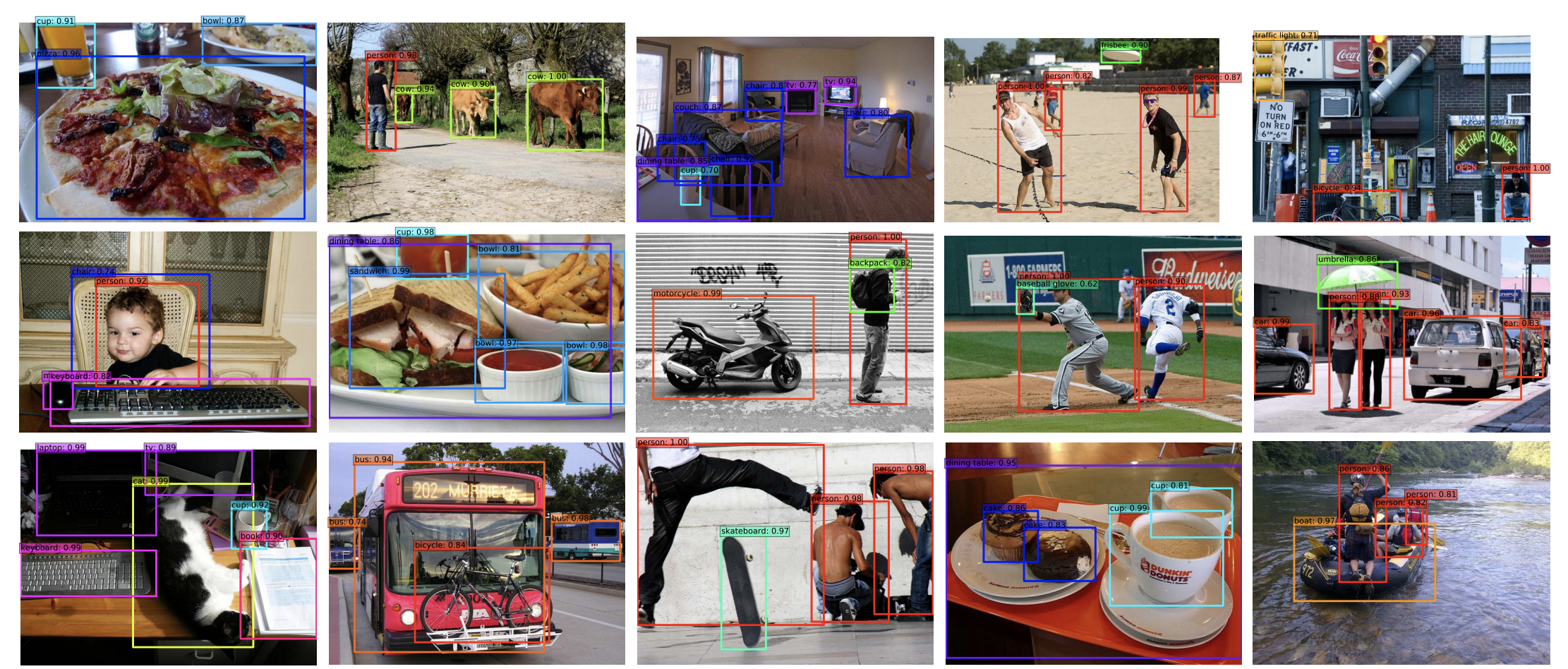
The SSD algorithm uses a CNN backbone, passes the input image through it and takes the convolutional outputs from different levels of the network. The list of these outputs are called feature maps. These feature maps are then passed through the Classification and Regression heads which are responsible for predicting the class and the location of the boxes.
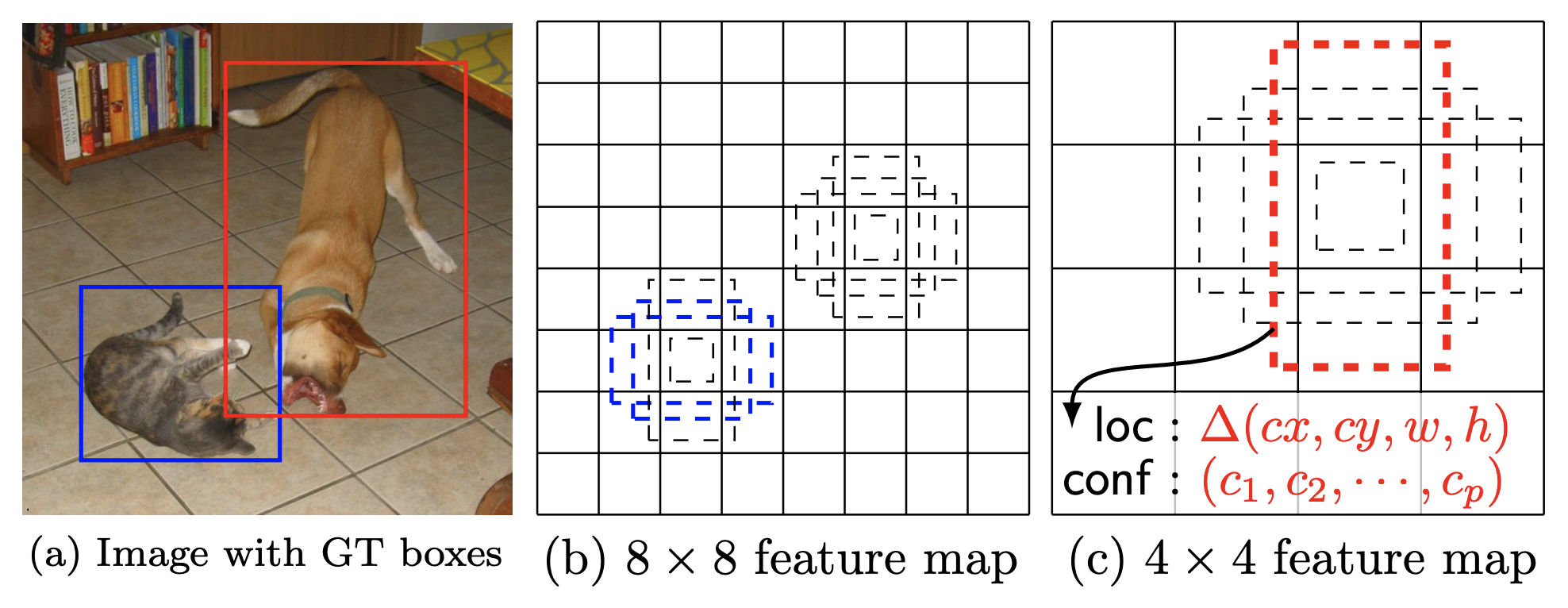
Since the feature maps of each image contain outputs from different levels of the network, their size varies and thus they can capture objects of different dimensions. On top of each, we tile several default boxes which can be thought as our rough prior guesses. For each default box, we predict whether there is an object (along with its class) and its offset (correction over the original location). During training time, we need to first match the ground truth to the default boxes and then we use those matches to estimate our loss. During inference, similar prediction boxes are combined to estimate the final predictions.
The SSD Network Architecture
In this section, we will discuss the key components of SSD. Our code follows closely the paper and makes use of many of the undocumented optimizations included in the official implementation.
DefaultBoxGenerator
The DefaultBoxGenerator class is responsible for generating the default boxes of SSD and operates similarly to the AnchorGenerator of FasterRCNN (for more info on their differences see pages 4-6 of the paper). It produces a set of predefined boxes of specific width and height which are tiled across the image and serve as the first rough prior guesses of where objects might be located. Here is Figure 1 from the SSD paper with a visualization of ground truths and default boxes:
The class is parameterized by a set of hyperparameters that control their shape and tiling. The implementation will provide automatically good guesses with the default parameters for those who want to experiment with new backbones/datasets but one can also pass optimized custom values.
SSDMatcher
The SSDMatcher class extends the standard Matcher used by FasterRCNN and it is responsible for matching the default boxes to the ground truth. After estimating the IoUs of all combinations, we use the matcher to find for each default box the best candidate ground truth with overlap higher than the IoU threshold. The SSD version of the matcher has an extra step to ensure that each ground truth is matched with the default box that has the highest overlap. The results of the matcher are used in the loss estimation during the training process of the model.
Classification and Regression Heads
The SSDHead class is responsible for initializing the Classification and Regression parts of the network. Here are a few notable details about their code:
- Both the Classification and the Regression head inherit from the same class which is responsible for making the predictions for each feature map.
- Each level of the feature map uses a separate 3×3 Convolution to estimate the class logits and box locations.
- The number of predictions that each head makes per level depends on the number of default boxes and the sizes of the feature maps.
Backbone Feature Extractor
The feature extractor reconfigures and enhances a standard VGG backbone with extra layers as depicted on the Figure 2 of the SSD paper:
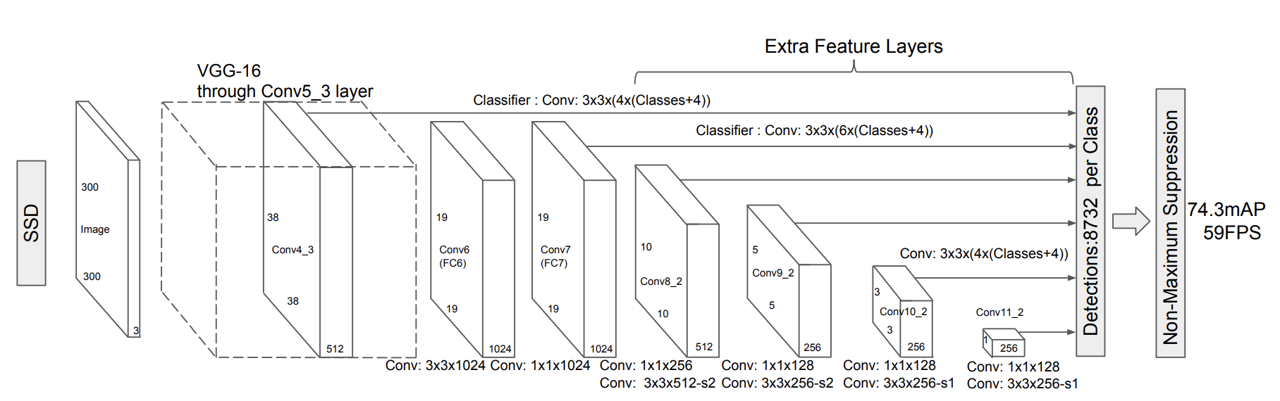
The class supports all VGG models of TorchVision and one can create a similar extractor class for other types of CNNs (see this example for ResNet). Here are a few implementation details of the class:
- Patching the
ceil_mode parameterof the 3rd Maxpool layer is necessary to get the same feature map sizes as the paper. This is due to small differences between PyTorch and the original Caffe implementation of the model. - It adds a series of extra feature layerson top of VGG. If the highres parameter is
Trueduring its construction, it will append an extra convolution. This is useful for the SSD512 version of the model. - As discussed on section 3 of the paper, the fully connected layers of the original VGG are converted to convolutions with the first one using Atrous. Moreover maxpool5’s stride and kernel size is modified.
- As described on section 3.1, L2 normalization is used on the output of conv4_3 and a set of learnable weights are introduced to control its scaling.
SSD Algorithm
The final key piece of the implementation is on the SSD class. Here are some notable details:
- The algorithm is parameterized by a set of arguments similar to other detection models. The mandatory parameters are: the backbone which is responsible for estimating the feature maps, the
anchor_generatorwhich should be a configured instance of theDefaultBoxGeneratorclass, the size to which the input images will be resized and thenum_classesfor classification excluding the background. - If a head is not provided, the constructor will initialize the default
SSDHead. To do so, we need to know the number of output channels for each feature map produced by the backbone. Initially we try to retrieve this information from the backbone but if not available we will dynamically estimate it. - The algorithm reuses the standard BoxCoder class used by other Detection models. The class is responsible for encoding and decoding the bounding boxes and is configured to use the same prior variances as the original implementation.
- Though we reuse the standard GeneralizedRCNNTransform class to resize and normalize the input images, the SSD algorithm configures it to ensure that the image size will remain fixed.
Here are the two core methods of the implementation:
- The
compute_lossmethod estimates the standard Multi-box loss as described on page 5 of the SSD paper. It uses the smooth L1 loss for regression and the standard cross-entropy loss with hard-negative sampling for classification. - As in all detection models, the forward method currently has different behaviour depending on whether the model is on training or eval mode. It starts by resizing & normalizing the input images and then passes them through the backbone to get the feature maps. The feature maps are then passed through the head to get the predictions and then the method generates the default boxes.
- If the model is on training mode, the forward will estimate the IoUs of the default boxes with the ground truth, use the
SSDmatcherto produce matches and finally estimate the losses by calling thecompute_loss method. - If the model is on eval mode, we first select the best detections by keeping only the ones that pass the score threshold, select the most promising boxes and run NMS to clean up and select the best predictions. Finally we postprocess the predictions to resize them to the original image size.
- If the model is on training mode, the forward will estimate the IoUs of the default boxes with the ground truth, use the
The SSD300 VGG16 Model
The SSD is a family of models because it can be configured with different backbones and different Head configurations. In this section, we will focus on the provided SSD pre-trained model. We will discuss the details of its configuration and the training process used to reproduce the reported results.
Training process
The model was trained using the COCO dataset and all of its hyper-parameters and scripts can be found in our references folder. Below we provide details on the most notable aspects of the training process.
Paper Hyperparameters
In order to achieve the best possible results on COCO, we adopted the hyperparameters described on the section 3 of the paper concerning the optimizer configuration, the weight regularization etc. Moreover we found it useful to adopt the optimizations that appear in the official implementation concerning the tiling configuration of the DefaultBox generator. This optimization was not described in the paper but it was crucial for improving the detection precision of smaller objects.
Data Augmentation
Implementing the SSD Data Augmentation strategy as described on page 6 and page 12 of the paper was critical to reproducing the results. More specifically the use of random “Zoom In” and “Zoom Out” transformations make the model robust to various input sizes and improve its precision on the small and medium objects. Finally since the VGG16 has quite a few parameters, the photometric distortions included in the augmentations have a regularization effect and help avoid the overfitting.
Weight Initialization & Input Scaling
Another aspect that we found beneficial was to follow the weight initialization scheme proposed by the paper. To do that, we had to adapt our input scaling method by undoing the 0-1 scaling performed by ToTensor() and use pre-trained ImageNet weights fitted with this scaling (shoutout to Max deGroot for providing them in his repo). All the weights of new convolutions were initialized using Xavier and their biases were set to zero. After initialization, the network was trained end-to-end.
LR Scheme
As reported on the paper, after applying aggressive data augmentations it’s necessary to train the models for longer. Our experiments confirm this and we had to tweak the Learning rate, batch sizes and overall steps to achieve the best results. Our proposed learning scheme is configured to be rather on the safe side, showed signs of plateauing between the steps and thus one is likely to be able to train a similar model by doing only 66% of our epochs.
Breakdown of Key Accuracy Improvements
It is important to note that implementing a model directly from a paper is an iterative process that circles between coding, training, bug fixing and adapting the configuration until we match the accuracies reported on the paper. Quite often it also involves simplifying the training recipe or enhancing it with more recent methodologies. It is definitely not a linear process where incremental accuracy improvements are achieved by improving a single direction at a time but instead involves exploring different hypothesis, making incremental improvements in different aspects and doing a lot of backtracking.
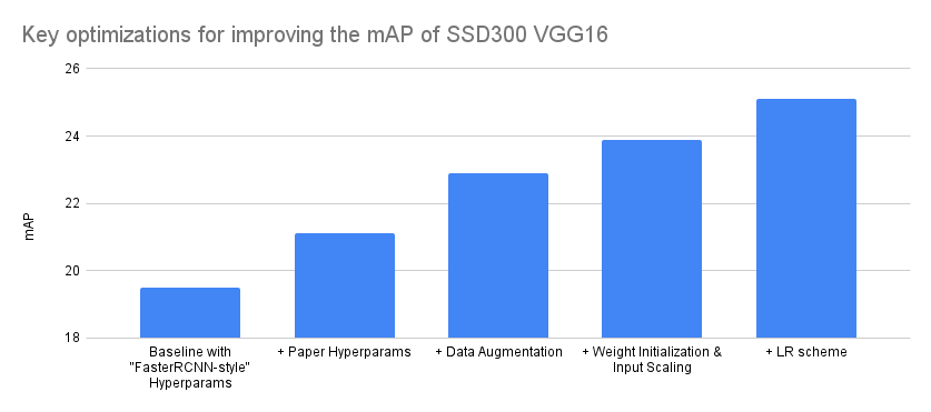
With that in mind, below we try to summarize the optimizations that affected our accuracy the most. We did this by grouping together the various experiments in 4 main groups and attributing the experiment improvements to the closest match. Note that the Y-axis of the graph starts from 18 instead from 0 to make the difference between optimizations more visible:
| Model Configuration | mAP delta | mAP |
|---|---|---|
| Baseline with “FasterRCNN-style” Hyperparams | – | 19.5 |
| + Paper Hyperparams | 1.6 | 21.1 |
| + Data Augmentation | 1.8 | 22.9 |
| + Weight Initialization & Input Scaling | 1 | 23.9 |
| + LR scheme | 1.2 | 25.1 |
Our final model achieves an mAP of 25.1 and reproduces exactly the COCO results reported on the paper. Here is a detailed breakdown of the accuracy metrics.
We hope you found the part 1 of the series interesting. On the part 2, we will focus on the implementation of SSDlite and discuss its differences from SSD. Until then, we are looking forward to your feedback.
A Step Toward More Inclusive People Annotations in the Open Images Extended Dataset
Posted by Candice Schumann and Susanna Ricco, Software Engineers, Google Research
In 2016, we introduced Open Images, a collaborative release of ~9 million images annotated with image labels spanning thousands of object categories and bounding box annotations for 600 classes. Since then, we have made several updates, including the release of crowdsourced data to the Open Images Extended collection to improve diversity of object annotations. While the labels provided with these datasets were expansive, they did not focus on sensitive attributes for people, which are critically important for many machine learning (ML) fairness tasks, such as fairness evaluations and bias mitigation. In fact, finding datasets that include thorough labeling of such sensitive attributes is difficult, particularly in the domain of computer vision.
Today, we introduce the More Inclusive Annotations for People (MIAP) dataset in the Open Images Extended collection. The collection contains more complete bounding box annotations for the person class hierarchy in 100k images containing people. Each annotation is also labeled with fairness-related attributes, including perceived gender presentation and perceived age range. With the increasing focus on reducing unfair bias as part of responsible AI research, we hope these annotations will encourage researchers already leveraging Open Images to incorporate fairness analysis in their research.
 |
| Examples of new boxes in MIAP. In each subfigure the magenta boxes are from the original Open Images dataset, while the yellow boxes are additional boxes added by the MIAP Dataset. Original photo credits — left: Boston Public Library; middle: jen robinson; right: Garin Fons; all used with permission under the CC- BY 2.0 license. |
Annotations in Open Images
Each image in the original Open Images dataset contains image-level annotations that broadly describe the image and bounding boxes drawn around specific objects. To avoid drawing multiple boxes around the same object, less specific classes were temporarily pruned from the label candidate set, a process that we refer to as hierarchical de-duplication. For example, an image with labels animal, cat, and washing machine has bounding boxes annotated for cat and washing machine, but not for the redundant class animal.
The MIAP dataset addresses the five classes that are part of the person hierarchy in the original Open Images dataset: person, man, woman, boy, girl. The existence of these labels make the Open Images dataset uniquely valuable for research advancing responsible AI, allowing one to train a general person detector with access to gender- and age-range-specific labels for fairness analysis and bias mitigation.
However, we found that the combination of hierarchical de-duplication and societally imposed distinctions between woman/girl and man/boy introduced limitations in the original annotations. For example, if annotators were asked to draw boxes for the class girl, they would not draw a box around a boy in the image. They may or may not draw a box around a woman depending on their assessment of the age of the individual and their cultural understanding of the concept of girl. These decisions could be applied inconsistently between images, depending on the cultural background of the individual annotator, the appearance of an individual, and the context of the scene. Consequently, the bounding box annotations in some images were incomplete, with some people who appeared prominently not being annotated.
Annotations in MIAP
The new MIAP annotations are designed to address these limitations and fulfill the promise of Open Images as a dataset that will enable new advances in machine learning fairness research. Rather than asking annotators to draw boxes for the most specific class from the hierarchy (e.g., girl), we invert the procedure, always requesting bounding boxes for the gender- and age-agnostic person class. All person boxes are then separately associated with labels for perceived gender presentation (predominantly feminine, predominantly masculine, or unknown) and age presentation (young, middle, older, or unknown). We recognize that gender is not binary and that an individual’s gender identity may not match their perceived or intended gender presentation and, in an effort to mitigate the effects of unconscious bias on the annotations, we reminded annotators that norms around gender expression vary across cultures and have changed over time.
This procedure adds a significant number of boxes that were previously missing.
Over the 100k images that include people, the number of person bounding boxes have increased from ~358k to ~454k. The number of bounding boxes per perceived gender presentation and perceived age presentation increased consistently. These new annotations provide more complete ground truth for training a person detector as well as more accurate subgroup labels for incorporating fairness into computer vision research.
 |
 |
| Comparison of number of person bounding boxes between the original Open Images and the new MIAP dataset. |
Intended Use
We include annotations for perceived age range and gender presentation for person bounding boxes because we believe these annotations are necessary to advance the ability to better understand and work to mitigate and eliminate unfair bias or disparate performance across protected subgroups within the field of image understanding. We note that the labels capture the gender and age range presentation as assessed by a third party based on visual cues alone, rather than an individual’s self-identified gender or actual age. We do not support or condone building or deploying gender and/or age presentation classifiers trained from these annotations as we believe the risks associated with the use of these technologies outside fairness research outweigh any potential benefits.
Acknowledgements
The core team behind this work included Utsav Prabhu, Vittorio Ferrari, and Caroline Pantofaru. We would also like to thank Alex Hanna, Reena Jana, Alina Kuznetsova, Matteo Malloci, Stefano Pellegrini, Jordi Pont-Tuset, and Mahima Pushkarna, for their contributions to the project.
Amazon teams up with Columbia University for research showcase
Register for the June 17 Annual Research Showcase organized by the Columbia Center of Artificial Intelligence.Read More
Voiceitt extends the voice revolution to people with nonstandard speech
Alexa Fund company unlocks voice-based computing for people who have trouble using their voices.Read More
New PyTorch Library Releases in PyTorch 1.9, including TorchVision, TorchAudio, and more
Today, we are announcing updates to a number of PyTorch libraries, alongside the PyTorch 1.9 release. The updates include new releases for the domain libraries including TorchVision, TorchText and TorchAudio. These releases, along with the PyTorch 1.9 release, include a number of new features and improvements that will provide a broad set of updates for the PyTorch community.
Some highlights include:
- TorchVision – Added new SSD and SSDLite models, quantized kernels for object detection, GPU Jpeg decoding, and iOS support. See release notes here.
- TorchAudio – Added wav2vec 2.0 model deployable in non-Python environments (including C++, Android, and iOS). Many performance improvements in lfilter, spectral operations, resampling. Added options for quality control in sampling (i.e. Kaiser window support). Initiated the migration of complex tensors operations. Improved autograd support. See release notes here.
- TorchText – Added a new high-performance Vocab module that provides common functional APIs for NLP workflows. See release notes here.
We’d like to thank the community for their support and work on this latest release.
Features in PyTorch releases are classified as Stable, Beta, and Prototype. You can learn more about the definitions in this blog post.
TorchVision 0.10
(Stable) Quantized kernels for object detection
The forward pass of the nms and roi_align operators now support tensors with a quantized dtype, which can help lower the memory footprint of object detection models, particularly on mobile environments. For more details, refer to the documentation.
(Stable) Speed optimizations for Tensor transforms
The resize and flip transforms have been optimized and its runtime improved by up to 5x on the CPU.
(Stable) Documentation improvements
Significant improvements were made to the documentation. In particular, a new gallery of examples is available. These examples visually illustrate how each transform acts on an image, and also properly documents and illustrates the output of the segmentation models.
The example gallery will be extended in the future to provide more comprehensive examples and serve as a reference for common torchvision tasks. For more details, refer to the documentation.
(Beta) New models for detection
SSD and SSDlite are two popular object detection architectures that are efficient in terms of speed and provide good results for low resolution pictures. In this release, we provide implementations for the original SSD model with VGG16 backbone and for its mobile-friendly variant SSDlite with MobileNetV3-Large backbone.
The models were pre-trained on COCO train2017 and can be used as follows:
import torch
import torchvision

# Original SSD variant
x = [torch.rand(3, 300, 300), torch.rand(3, 500, 400)]
m_detector = torchvision.models.detection.ssd300_vgg16(pretrained=True)
m_detector.eval()
predictions = m_detector(x)

# Mobile-friendly SSDlite variant
x = [torch.rand(3, 320, 320), torch.rand(3, 500, 400)]
m_detector = torchvision.models.detection.ssdlite320_mobilenet_v3_large(pretrained=True)
m_detector.eval()
predictions = m_detector(x)
The following accuracies can be obtained on COCO val2017 (full results available in #3403 and #3757):
| Model | mAP | mAP@50 | mAP@75 |
|---|---|---|---|
| SSD300 VGG16 | 25.1 | 41.5 | 26.2 |
| SSDlite320 MobileNetV3-Large | 21.3 | 34.3 | 22.1 |
For more details, refer to the documentation.
(Beta) JPEG decoding on the GPU
Decoding jpegs is now possible on GPUs with the use of nvjpeg, which should be readily available in your CUDA setup. The decoding time of a single image should be about 2 to 3 times faster than with libjpeg on CPU. While the resulting tensor will be stored on the GPU device, the input raw tensor still needs to reside on the host (CPU), because the first stages of the decoding process take place on the host:
from torchvision.io.image import read_file, decode_jpeg
data = read_file('path_to_image.jpg')  # raw data is on CPU
img = decode_jpeg(data, device='cuda')  # decoded image in on GPU
For more details, see the documentation.
(Beta) iOS support
TorchVision 0.10 now provides pre-compiled iOS binaries for its C++ operators, which means you can run Faster R-CNN and Mask R-CNN on iOS. An example app on how to build a program leveraging those ops can be found here.
TorchAudio 0.9.0
(Stable) Complex Tensor Migration
TorchAudio has functions that handle complex-valued tensors. These functions follow a convention to use an extra dimension to represent real and imaginary parts. In PyTorch 1.6, the native complex type was introduced. As its API is getting stable, torchaudio has started to migrate to the native complex type.
In this release, we added support for native complex tensors, and you can opt-in to use them. Using the native complex types, we have verified that affected functions continue to support autograd and TorchScript, moreover, switching to native complex types improves their performance. For more details, refer to pytorch/audio#1337.
(Stable) Filtering Improvement
In release 0.8, we added the C++ implementation of the core part of lfilter for CPU, which improved the performance. In this release, we optimized some internal operations of the CPU implementation for further performance improvement. We also added autograd support to both CPU and GPU. Now lfilter and all the biquad filters (biquad, band_biquad, bass_biquad, treble_biquad, allpass_biquad, lowpass_biquad, highpass_biquad, bandpass_biquad, equalizer_biquad and bandrefect_biquad) benefit from the performance improvement and support autograd. We also moved the implementation of overdrive to C++ for performance improvement. For more details, refer to the documentation.
(Stable) Improved Autograd Support
Along with the work of Complex Tensor Migration and Filtering Improvement, we also added autograd tests to transforms. lfilter, biquad and its variants, and most transforms are now guaranteed to support autograd. For more details, refer to the release note.
(Stable) Improved Windows Support
Torchaudio implements some operations in C++ for reasons such as performance and integration with third-party libraries. These C++ components were only available on Linux and macOS. In this release, we have added support to Windows. With this, the efficient filtering implementation mentioned above is also available on Windows.
However, please note that not all the C++ components are available for Windows. “sox_io” backend and torchaudio.functional.compute_kaldi_pitch are not supported.
(Stable) I/O Functions Migration
Since the 0.6 release, we have continuously improved I/O functionality. Specifically, in 0.8 we changed the default backend from “sox” to “sox_io” and applied the same switch to API of the “soundfile” backend. The 0.9 release concludes this migration by removing the deprecated backends. For more details, please refer to #903.
(Beta) Wav2Vec2.0 Model
We have added the model architectures from Wav2Vec2.0. You can import fine-tuned models parameters published on fairseq and Hugging Face Hub. Our model definition supports TorchScript, and it is possible to deploy the model to non-Python environments, such as C++, Android and iOS.
The following code snippet illustrates such a use case. Please check out our c++ example directory for the complete example. Currently, it is designed for running inference. If you would like more support for training, please file a feature request.
# Import fine-tuned model from Hugging Face Hub
import transformers
from torchaudio.models.wav2vec2.utils import import_huggingface_model

original = Wav2Vec2ForCTC.from_pretrained("facebook/wav2vec2-base-960h")
imported = import_huggingface_model(original)
# Import fine-tuned model from fairseq
import fairseq
from torchaudio.models.wav2vec2.utils import import_fairseq_model

original, _, _ = fairseq.checkpoint_utils.load_model_ensemble_and_task(
    ["wav2vec_small_960h.pt"], arg_overrides={'data': "<data_dir>"})
imported = import_fairseq_model(original[0].w2v_encoder)
# Build uninitialized model and load state dict
from torchaudio.models import wav2vec2_base

model = wav2vec2_base(num_out=32)
model.load_state_dict(imported.state_dict())

# Quantize / script / optimize for mobile
quantized_model = torch.quantization.quantize_dynamic(
    model, qconfig_spec={torch.nn.Linear}, dtype=torch.qint8)
scripted_model = torch.jit.script(quantized_model)
optimized_model = optimize_for_mobile(scripted_model)
optimized_model.save("model_for_deployment.pt")
For more details, see the documentation.
(Beta) Resampling Improvement
In release 0.8, we vectorized the operation in torchaudio.compliance.kaldi.resample_waveform, which improved the performance of resample_waveform and torchaudio.transforms.Resample. In this release, we have further revised the way the resampling algorithm is implemented.
We have:
- Added Kaiser Window support for a wider range of resampling quality.
- Added
rolloffparameter for anti-aliasing control. - Added the mechanism to precompute the kernel and cache it in
torchaudio.transforms.Resamplefor even faster operation. - Moved the implementation from
torchaudio.compliance.kaldi.resample_waveformtotorchaudio.functional.resampleand deprecatedtorchaudio.compliance.kaldi.resample_waveform.
For more details, see the documentation.
(Prototype) RNN Transducer Loss
The RNN transducer loss is used in training RNN transducer models, which is a popular architecture for speech recognition tasks. The prototype loss in torchaudio currently supports autograd, torchscript, float16 and float32, and can also be run on both CPU and CUDA. For more details, please refer to the documentation.
TorchText 0.10.0
(Beta) New Vocab Module
In this release, we introduce a new Vocab module that replaces the current Vocab class. The new Vocab provides common functional APIs for NLP workflows. This module is backed by an efficient C++ implementation that reduces batch look-up time by up-to ~85% (refer to summary of #1248 and #1290 for further information on benchmarks), and provides support for TorchScript. We provide accompanying factory functions that can be used to build the Vocab object either through a python ordered dictionary or an Iterator that yields lists of tokens.
#creating Vocab from text file
import io
from torchtext.vocab import build_vocab_from_iterator
#generator that yield list of tokens
def yield_tokens(file_path):
   with io.open(file_path, encoding = 'utf-8') as f:
      for line in f:
          yield line.strip().split()
#get Vocab object
vocab_obj = build_vocab_from_iterator(yield_tokens(file_path), specials=["<unk>"])

#creating Vocab through ordered dict
from torchtext.vocab import vocab
from collections import Counter, OrderedDict
counter = Counter(["a", "a", "b", "b", "b"])
sorted_by_freq_tuples = sorted(counter.items(), key=lambda x: x[1], reverse=True)
ordered_dict = OrderedDict(sorted_by_freq_tuples)
vocab_obj = vocab(ordered_dict)

#common API usage

#look-up index
vocab_obj["a"]

#batch look-up indices
vocab_obj.looup_indices(["a","b"])
#support forward API of PyTorch nn Modules
vocab_obj(["a","b"])

#batch look-up tokens
vocab_obj.lookup_tokens([0,1])

#set default index to return when token not found
vocab_obj.set_default_index(0)
vocab_obj["out_of_vocabulary"] #prints 0
For more details, refer to the documentation.
Thanks for reading. If you’re interested in these updates and want to join the PyTorch community, we encourage you to join the discussion forums and open GitHub issues. To get the latest news from PyTorch, follow us on Facebook, Twitter, Medium, YouTube or LinkedIn.
Cheers!
-Team PyTorch