Proposal submissions for the third round of fairness in AI research are due August 3.Read More
Using Variational Transformer Networks to Automate Document Layout Design
Posted by Diego Martin Arroyo, Software Engineer and Federico Tombari, Research Scientist, Google Research
Information in a written document is not only conveyed by the meaning of the words contained in it, but also by the overall document layout. Layouts are commonly used to direct the order in which the reader parses a document to enable a better understanding (e.g., with columns or paragraphs), to provide helpful summaries (e.g., with titles) or for aesthetic purposes (e.g., when displaying advertisements).
While these design rules are easy to follow, it is difficult to explicitly define them without quickly needing to include exceptions or encountering ambiguous cases. This makes the automation of document design difficult, as any system with a hardcoded set of production rules will either be overly simplistic and thus incapable of producing original layouts (causing a lack of diversity in the layout of synthesized data), or too complex, with a large set of rules and their accompanying exceptions. In an attempt to solve this challenge, some have proposed machine learning (ML) techniques to synthesize document layouts. However, most ML-based solutions for automatic document design do not scale to a large number of layout components, or they rely on additional information for training, such as the relationships between the different components of a document.
In “Variational Transformer Networks for Layout Generation”, to be presented at CVPR 2021, we create a document layout generation system that scales to an arbitrarily large number of elements and does not require any additional information to capture the relationships between design elements. We use self-attention layers as building blocks of a variational autoencoder (VAE), which is able to model document layout design rules as a distribution, rather than using a set of predetermined heuristics, increasing the diversity of the generated layouts. The resulting Variational Transformer Network (VTN) model is able to extract meaningful relationships between the layout elements (paragraphs, tables, images, etc.), resulting in realistic synthetic documents (e.g., better alignment and margins). We show the effectiveness of this combination across different domains, such as scientific papers, UI layouts, and even furniture arrangements.
VAEs for Layout Generation
The ultimate goal of this system is to infer the design rules for a given type of layout from a collection of examples. If one considers these design rules as the distribution underlying the data, it is possible to use probabilistic models to discover it. We propose doing this with a VAE (widely used for tasks like image generation or anomaly detection), an autoencoder architecture that consists of two distinct subparts, the encoder and decoder. The encoder learns to compress the input to fewer dimensions, retaining only the necessary information to reconstruct the input, while the decoder learns to undo this operation. The compressed representation (also called the bottleneck) can be forced to behave like a known distribution (e.g., a uniform Gaussian). Feeding samples from this a priori distribution to the decoder segment of the network results in outputs similar to the training data.
An additional advantage of the VAE formulation is that it is agnostic to the type of operations used to implement the encoder and decoder segments. As such, we use self-attention layers (typically seen in Transformer architectures) to automatically capture the influence that each layout element has over the rest.
Transformers use self-attention layers to model long, sequenced relationships, often applied to an array of natural language understanding tasks, such as translation and summarization, as well as beyond the language domain in object detection or document layout understanding tasks. The self-attention operation relates every element in a sequence to every other and determines how they influence each other. This property is ideal to model relationships across different elements in a layout without the need for explicit annotations.
In order to synthesize new samples from these relationships, some approaches for layout generation [e.g., 1] and even for other domains [e.g., 2, 3] rely on greedy search algorithms, such as beam search, nucleus sampling or top-k sampling. Since these strategies are often based on exploration rules that tend to favor the most likely outcome at every step, the diversity of the generated samples is not guaranteed. However, by combining self-attention with the VAE’s probabilistic techniques, the model is able to directly learn a distribution from which it can extract new elements.
Modeling the Variational Bottleneck
The bottleneck of a VAE is commonly modeled as a vector representing the input. Since self-attention layers are a sequence-to-sequence architecture, i.e., a sequence of n input elements is mapped onto n output elements, the standard VAE formulation is difficult to apply. Inspired by BERT, we append an auxiliary token to the beginning of the sequence and treat it as the autoencoder bottleneck vector z. During training, the vector associated with this token is the only piece of information passed to the decoder, so the encoder needs to learn how to compress the entire document information in this vector. The decoder then learns to infer the number of elements in the document as well as the locations of each element in the input sequence from this vector alone. This strategy allows us to use standard techniques to regularize the bottleneck, such as the KL divergence.
Decoding
In order to synthesize documents with varying numbers of elements, the network needs to model sequences of arbitrary length, which is not trivial. While self-attention enables the encoder to adapt automatically to any number of elements, the decoder segment does not know the number of elements in advance. We overcome this issue by decoding sequences in an autoregressive way — at every step, the decoder produces an element, which is concatenated to the previously decoded elements (starting with the bottleneck vector z as input), until a special stop element is produced.
 |
| A visualization of our proposed architecture |
Turning Layouts into Input Data
A document is often composed of several design elements, such as paragraphs, tables, images, titles, footnotes, etc. In terms of design, layout elements are often represented by the coordinates of their enclosing bounding boxes. To make this information easily digestible for a neural network, we define each element with four variables (x, y, width, height), representing the element’s location on the page (x, y) and size (width, height).
Results
We evaluate the performance of the VTN following two criteria: layout quality and layout diversity. We train the model on publicly available document datasets, such as PubLayNet, a collection of scientific papers with layout annotations, and evaluate the quality of generated layouts by quantifying the amount of overlap and alignment between elements. We measure how well the synthetic layouts resemble the training distribution using the Wasserstein distance over the distributions of element classes (e.g., paragraphs, images, etc.) and bounding boxes. In order to capture the layout diversity, we find the most similar real sample for each generated document using the DocSim metric, where a higher number of unique matches to the real data indicates a more diverse outcome.
We compare the VTN approach to previous works like LayoutVAE and Gupta et al. The former is a VAE-based formulation with an LSTM backbone, whereas Gupta et al. use a self-attention mechanism similar to ours, combined with standard search strategies (beam search). The results below show that LayoutVAE struggles to comply with design rules, like strict alignments, as in the case of PubLayNet. Thanks to the self-attention operation, Gupta et al. can model these constraints much more effectively, but the usage of beam search affects the diversity of the results.
| IoU | Overlap | Alignment | Wasserstein Class ↓ | Wasserstein Box ↓ | # Unique Matches ↑ | |
| LayoutVAE | 0.171 | 0.321 | 0.472 | – | 0.045 | 241 |
| Gupta et al. | 0.039 | 0.006 | 0.361 | 0.018 | 0.012 | 546 |
| VTN | 0.031 | 0.017 | 0.347 | 0.022 | 0.012 | 697 |
| Real Data | 0.048 | 0.007 | 0.353 | – | – | – |
| Results on PubLayNet. Down arrows (↓) indicate that a lower score is better, whereas up arrows (↑) indicate higher is better. |
We also explore the ability of our approach to learn design rules in other domains, such as Android UIs (RICO), natural scenes (COCO) and indoor scenes (SUN RGB-D). Our method effectively learns the design rules of these datasets and produces synthetic layouts of similar quality as the current state of the art and a higher degree of diversity.
| IoU | Overlap | Alignment | Wasserstein Class ↓ | Wasserstein Box ↓ | # Unique Matches ↑ | |
| LayoutVAE | 0.193 | 0.400 | 0.416 | – | 0.045 | 496 |
| Gupta et al. | 0.086 | 0.145 | 0.366 | 0.004 | 0.023 | 604 |
| VTN | 0.115 | 0.165 | 0.373 | 0.007 | 0.018 | 680 |
| Real Data | 0.084 | 0.175 | 0.410 | – | – | – |
| Results on RICO. Down arrows (↓) indicate that a lower score is better, whereas up arrows (↑) indicate higher is better. |
| IoU | Overlap | Alignment | Wasserstein Class ↓ | Wasserstein Box ↓ | # Unique Matches ↑ | |
| LayoutVAE | 0.325 | 2.819 | 0.246 | – | 0.062 | 700 |
| Gupta et al. | 0.194 | 1.709 | 0.334 | 0.001 | 0.016 | 601 |
| VTN | 0.197 | 2.384 | 0.330 | 0.0005 | 0.013 | 776 |
| Real Data | 0.192 | 1.724 | 0.347 | – | – | – |
| Results for COCO. Down arrows (↓) indicate that a lower score is better, whereas up arrows (↑) indicate higher is better. |
Below are some examples of layouts produced by our method compared to existing methods. The design rules learned by the network (location, margins, alignment) resemble those of the original data and show a high degree of variability.
| LayoutVAE |
 |
| Gupta et al. |
 |
| VTN |
 |
| Qualitative results of our method on PubLayNet compared to existing state-of-the-art methods. |
Conclusion
In this work we show the feasibility of using self-attention as part of the VAE formulation. We validate the effectiveness of this approach for layout generation, achieving state-of-the-art performance on various datasets and across different tasks. Our research paper also explores alternative architectures for the integration of self-attention and VAEs, exploring non-autoregressive decoding strategies and different types of priors, and analyzes advantages and disadvantages. The layouts produced by our method can help to create synthetic training data for downstream tasks, such as document parsing or automating graphic design tasks. We hope that this work provides a foundation for continued research in this area, as many subproblems are still not completely solved, such as how to suggest styles for the elements in the layout (text font, which image to choose, etc.) or how to reduce the amount of training data necessary for the model to generalize.
AcknowledgementsWe thank our co-author Janis Postels, as well as Alessio Tonioni and Luca Prasso for helping with the design of several of our experiments. We also thank Tom Small for his help creating the animations for this post.

Overview of PyTorch Autograd Engine
This blog post is based on PyTorch version 1.8, although it should apply for older versions too, since most of the mechanics have remained constant.
To help understand the concepts explained here, it is recommended that you read the awesome blog post by @ezyang: PyTorch internals if you are not familiar with PyTorch architecture components such as ATen or c10d.
What is autograd?
Background
PyTorch computes the gradient of a function with respect to the inputs by using automatic differentiation. Automatic differentiation is a technique that, given a computational graph, calculates the gradients of the inputs. Automatic differentiation can be performed in two different ways; forward and reverse mode. Forward mode means that we calculate the gradients along with the result of the function, while reverse mode requires us to evaluate the function first, and then we calculate the gradients starting from the output. While both modes have their pros and cons, the reverse mode is the de-facto choice since the number of outputs is smaller than the number of inputs, which allows a much more efficient computation. Check [3] to learn more about this.
Automatic differentiation relies on a classic calculus formula known as the chain-rule. The chain rule allows us to calculate very complex derivatives by splitting them and recombining them later.
Formally speaking, given a composite function , we can calculate its derivative as
. This result is what makes automatic differentiation work.
By combining the derivatives of the simpler functions that compose a larger one, such as a neural network, it is possible to compute the exact value of the gradient at a given point rather than relying on the numerical approximation, which would require multiple perturbations in the input to obtain a value.
To get the intuition of how the reverse mode works, let’s look at a simple function . Figure 1 shows its computational graph where the inputs x, y in the left, flow through a series of operations to generate the output z.
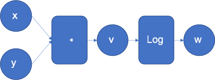
Figure 1: Computational graph of f(x, y) = log(x*y)
The automatic differentiation engine will normally execute this graph. It will also extend it to calculate the derivatives of w with respect to the inputs x, y, and the intermediate result v.
The example function can be decomposed in f and g, where and
. Every time the engine executes an operation in the graph, the derivative of that operation is added to the graph to be executed later in the backward pass. Note, that the engine knows the derivatives of the basic functions.
In the example above, when multiplying x and y to obtain v, the engine will extend the graph to calculate the partial derivatives of the multiplication by using the multiplication derivative definition that it already knows. and
. The resulting extended graph is shown in Figure 2, where the MultDerivative node also calculates the product of the resulting gradients by an input gradient to apply the chain rule; this will be explicitly seen in the following operations. Note that the backward graph (green nodes) will not be executed until all the forward steps are completed.
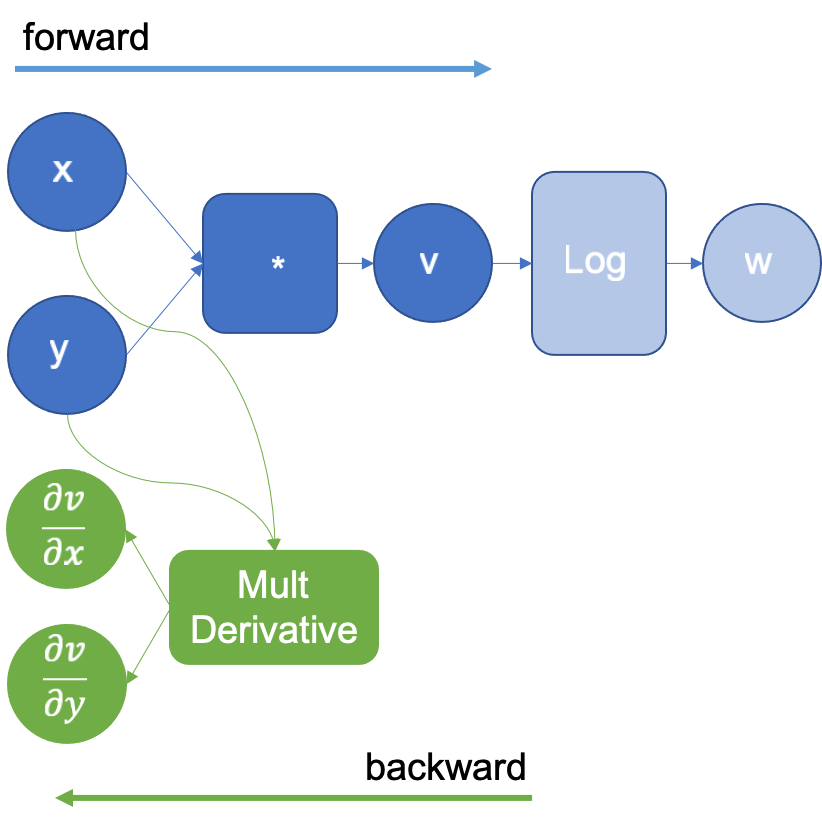
Figure 2: Computational graph extended after executing the logarithm
Continuing, the engine now calculates the operation and extends the graph again with the log derivative that it knows to be
. This is shown in figure 3. This operation generates the result
that when propagated backward and multiplied by the multiplication derivative as in the chain rule, generates the derivatives
,
.
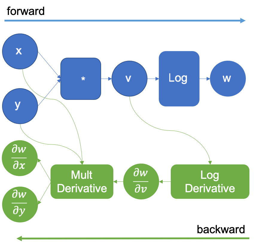
Figure 3: Computational graph extended after executing the logarithm
The original computation graph is extended with a new dummy variable z that is the same w. The derivative of z with respect to w is 1 as they are the same variable, this trick allows us to apply the chain rule to calculate the derivatives of the inputs. After the forward pass is complete, we start the backward pass, by supplying the initial value of 1.0 for . This is shown in Figure 4.
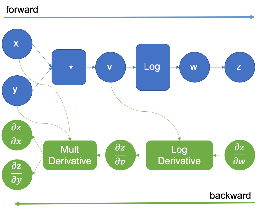
Figure 4: Computational graph extended for reverse auto differentiation
Then following the green graph we execute the LogDerivative operation that the auto differentiation engine introduced, and multiply its result by
to obtain the gradient
as per the chain rule states. Next, the multiplication derivative is executed in the same way, and the desired derivatives
are finally obtained.
Formally, what we are doing here, and PyTorch autograd engine also does, is computing a Jacobian-vector product (Jvp) to calculate the gradients of the model parameters, since the model parameters and inputs are vectors.
The Jacobian-vector product
When we calculate the gradient of a vector-valued function (a function whose inputs and outputs are vectors), we are essentially constructing a Jacobian matrix .
Thanks to the chain rule, multiplying the Jacobian matrix of a function by a vector
with the previously calculated gradients of a scalar function
results in the gradients
of the scalar output with respect to the vector-valued function inputs.
As an example, let’s look at some functions in python notation to show how the chain rule applies.
def f(x1, x2):
      a = x1 * x2
      y1 = log(a)
      y2 = sin(x2)
      return (y1, y2)
def g(y1, y2):
      return y1 * y2
Now, if we derive this by hand using the chain rule and the definition of the derivatives, we obtain the following set of identities that we can directly plug into the Jacobian matrix of
Next, let’s consider the gradients for the scalar function
If we now calculate the transpose-Jacobian vector product obeying the chain rule, we obtain the following expression:
Evaluating the Jvp for yields the result:
We can execute the same expression in PyTorch and calculate the gradient of the input:
>>> import torch
>>> x = torch.tensor([0.5, 0.75], requires_grad=True)
>>> y = torch.log(x[0] * x[1]) * torch.sin(x[1])
>>> y.backward(1.0)
>>> x.grad
tensor([1.3633,
0.1912])</pre>
The result is the same as our hand-calculated Jacobian-vector product!
However, PyTorch never constructed the matrix as it could grow prohibitively large but instead, created a graph of operations that traversed backward while applying the Jacobian-vector products defined in tools/autograd/derivatives.yaml.
Going through the graph
Every time PyTorch executes an operation, the autograd engine constructs the graph to be traversed backward.
The reverse mode auto differentiation starts by adding a scalar variable at the end so that
as we saw in the introduction. This is the initial gradient value that is supplied to the Jvp engine calculation as we saw in the section above.
In PyTorch, the initial gradient is explicitly set by the user when he calls the backward method.
Then, the Jvp calculation starts but it never constructs the matrix. Instead, when PyTorch records the computational graph, the derivatives of the executed forward operations are added (Backward Nodes). Figure 5 shows a backward graph generated by the execution of the functions and
seen before.
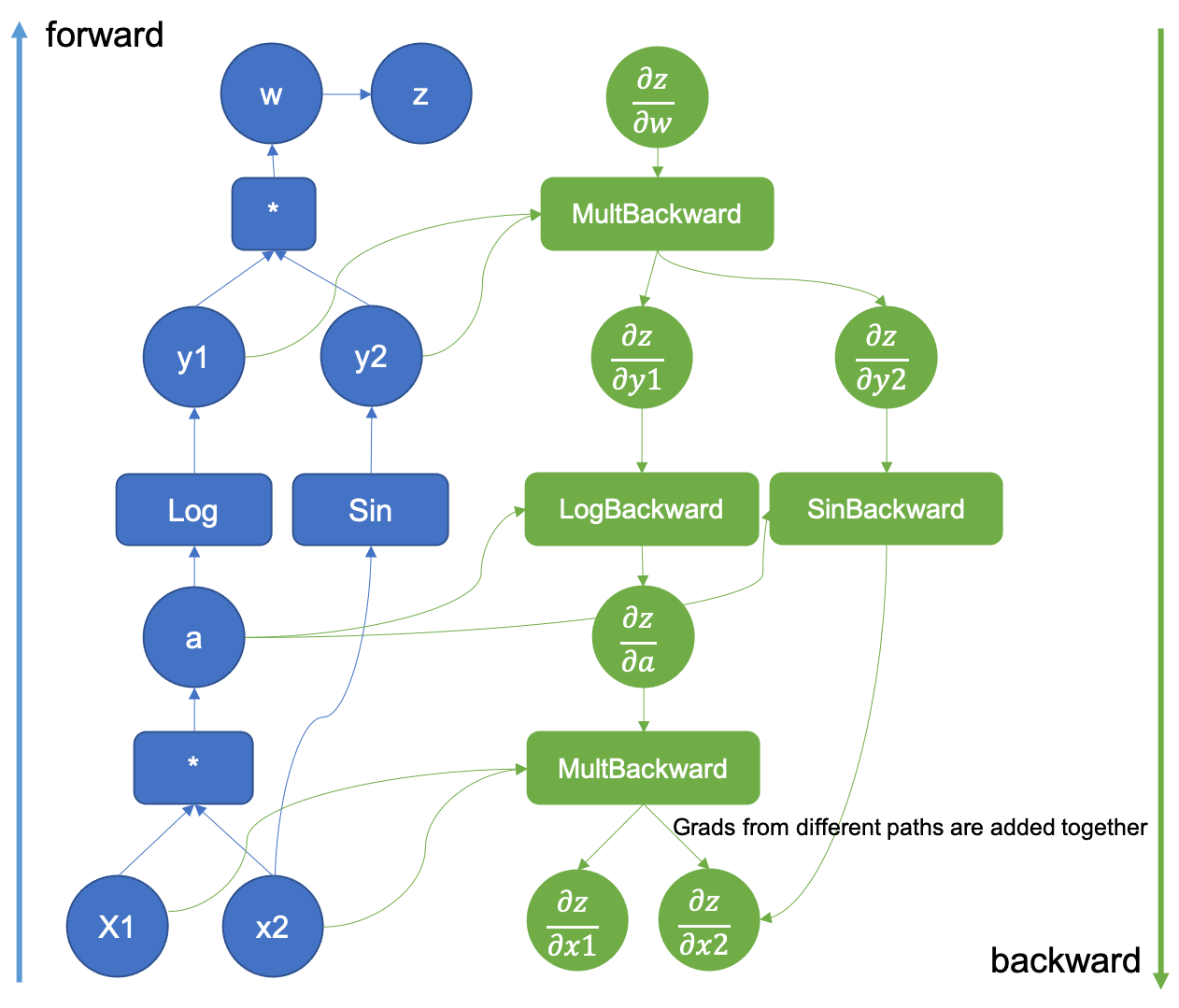
Figure 5: Computational Graph extended with the backward pass
Once the forward pass is done, the results are used in the backward pass where the derivatives in the computational graph are executed. The basic derivatives are stored in the tools/autograd/derivatives.yaml file and they are not regular derivatives but the Jvp versions of them [3]. They take their primitive function inputs and outputs as parameters along with the gradient of the function outputs with respect to the final outputs. By repeatedly multiplying the resulting gradients by the next Jvp derivatives in the graph, the gradients up to the inputs will be generated following the chain rule.
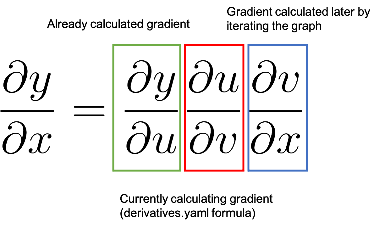
Figure 6: How the chain rule is applied in backward differentiation
Figure 6 represents the process by showing the chain rule. We started with a value of 1.0 as detailed before which is the already calculated gradient highlighted in green. And we move to the next node in the graph. The backward function registered in derivatives.yaml will calculate the associated
value highlighted in red and multiply it by
. By the chain rule this results in
which will be the already calculated gradient (green) when we process the next backward node in the graph.
You may also have noticed that in Figure 5 there is a gradient generated from two different sources. When two different functions share an input, the gradients with respect to the output are aggregated for that input, and calculations using that gradient can’t proceed unless all the paths have been aggregated together.
Let’s see an example of how the derivatives are stored in PyTorch.
Suppose that we are currently processing the backward propagation of the function, in the LogBackward node in Figure 2. The derivative of
in
derivatives.yaml is specified as grad.div(self.conj()). grad is the already calculated gradient and
self.conj() is the complex conjugate of the input vector. For complex numbers PyTorch calculates a special derivative called the conjugate Wirtinger derivative [6]. This derivative takes the complex number and its conjugate and by operating some magic that is described in [6], they are the direction of steepest descent when plugged into optimizers.
This code translates to , the corresponding green, and red squares in Figure 3. Continuing, the autograd engine will execute the next operation; backward of the multiplication. As before, the inputs are the original function’s inputs and the gradient calculated from the
backward step. This step will keep repeating until we reach the gradient with respect to the inputs and the computation will be finished. The gradient of
is only completed once the multiplication and sin gradients are added together. As you can see, we computed the equivalent of the Jvp but without constructing the matrix.
In the next post we will dive inside PyTorch code to see how this graph is constructed and where are the relevant pieces should you want to experiment with it!
References
- https://pytorch.org/tutorials/beginner/blitz/autograd_tutorial.html
- https://web.stanford.edu/class/cs224n/readings/gradient-notes.pdf
- https://www.cs.toronto.edu/~rgrosse/courses/csc321_2018/slides/lec10.pdf
- https://mustafaghali11.medium.com/how-pytorch-backward-function-works-55669b3b7c62
- https://indico.cern.ch/event/708041/contributions/3308814/attachments/1813852/2963725/automatic_differentiation_and_deep_learning.pdf
- https://pytorch.org/docs/stable/notes/autograd.html#complex-autograd-doc
- cs.ubc.ca/~fwood/CS340/lectures/AD1.pdf
Recommended: shows why the backprop is formally expressed with the Jacobian
PluggableDevice: Device Plugins for TensorFlow
Posted by Penporn Koanantakool and Pankaj Kanwar.
As the number of accelerators (GPUs, TPUs) in the ML ecosystem has exploded, there has been a strong need for seamless integration of new accelerators with TensorFlow. In this post, we introduce the PluggableDevice architecture which offers a plugin mechanism for registering devices with TensorFlow without the need to make changes in TensorFlow code.
This PluggableDevice architecture has been designed & developed collaboratively within the TensorFlow community. It leverages the work done for Modular TensorFlow, and is built using the StreamExecutor C API. The PluggableDevice mechanism is available in TF 2.5.
The need for Seamless integration
Prior to this, any integration of a new device required changes to the core TensorFlow. This was not scalable because of several issues, for example:
- Complex build dependencies and compiler toolchains. Onboarding a new compiler is nontrivial and adds to the technical complexity of the product.
- Slow development time. Changes need code reviews from the TensorFlow team, which can take time. Added technical complexity also adds to the development and testing time for new features.
- Combinatorial number of build configurations to test for. The changes made for a particular device might affect other devices or other components of TensorFlow. Each new device could increase the number of test configurations in a multiplicative manner.
- Easy to break. The lack of a contract via a well defined API means that it’s easier to break a particular device.
What is PluggableDevice?
The PluggableDevice mechanism requires no device-specific changes in the TensorFlow code. It relies on C APIs to communicate with the TensorFlow binary in a stable manner. Plug-in developers maintain separate code repositories and distribution packages for their plugins and are responsible for testing their devices. This way, TensorFlow’s build dependencies, toolchains, and test process are not affected. The integration is also less brittle since only changes to the C APIs or PluggableDevice components could affect the code.
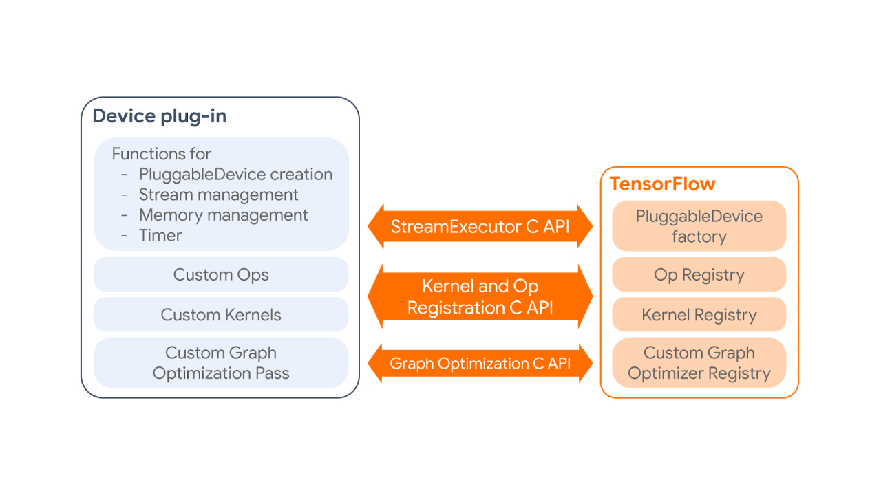
The PluggableDevice mechanism has four main components:
- PluggableDevice type: A new device type in TensorFlow which allows device registration from plug-in packages. It takes priority over native devices during the device placement phase.
- Custom operations and kernels: Plug-ins register their own operations and kernels to TensorFlow through the Kernel and Op Registration C API.
- Device execution and memory management: TensorFlow manages plug-in devices through the StreamExecutor C API.
- Custom graph optimization pass: Plug-ins can register one custom graph optimization pass, which will be run after all standard Grappler passes, through the Graph Optimization C API.
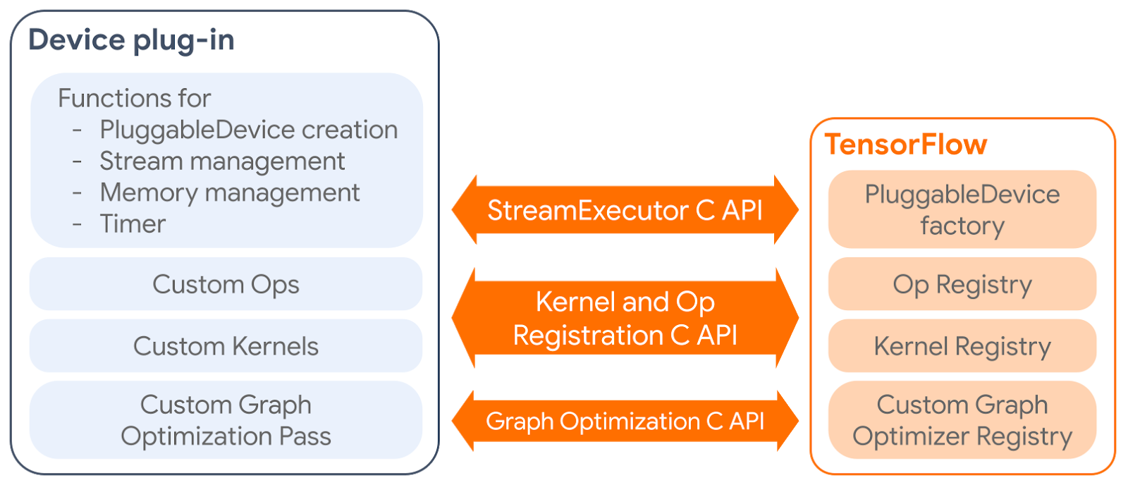 |
| How a device plug-in interacts with TensorFlow. |
Using PluggableDevice
To be able to use a particular device, like one would a native device in TensorFlow, users only have to install the device plug-in package for that device. The following code snippet shows how the plugin for a new device, say Awesome Processing Unit (APU), would be installed and used. For simplicity, let this APU plug-in only have one custom kernel for ReLU.
$ pip install tensorflow-apu-0.0.1-cp36-cp36m-linux_x86_64.whl
…
Successfully installed tensorflow-apu-0.0.1
$ python
Python 3.6.9 (default, Oct  8 2020, 12:12:24)
[GCC 8.4.0] on linux
Type "help", "copyright", "credits" or "license" for more information.
>>> import tensorflow as tf  # TensorFlow registers PluggableDevices here
>>> tf.config.list_physical_devices()
[PhysicalDevice(name='/physical_device:CPU:0', device_type='CPU'), PhysicalDevice(name='/physical_device:APU:0', device_type='APU')]

>>> a = tf.random.normal(shape=[5], dtype=tf.float32)  # Runs on CPU
>>> b =  tf.nn.relu(a)  # Runs on APU

>>> with tf.device("/APU:0"):  # Users can also use 'with tf.device' syntax
...  c = tf.nn.relu(a)  # Runs on APU

>>> @tf.function  # Defining a tf.function
... def run():
...    d = tf.random.uniform(shape=[100], dtype=tf.float32)  # Runs on CPU
...    e = tf.nn.relu(d)  # Runs on APU
>>> run()  # PluggableDevices also work with tf.function and graph mode.
Upcoming PluggableDevices
We are excited to announce that Intel will be one of our first partners to release a PluggableDevice. Intel has made significant contributions to this effort, submitting over 3 RFCs implementing the overall mechanism. They will release an Intel extension for TensorFlow (ITEX) plugin package to bring Intel XPU to TensorFlow for AI workload acceleration. We also expect other partners to take advantage of PluggableDevice and release additional plug-ins.
We will publish a detailed tutorial on how to develop a PluggableDevice plug-in for partners who might be interested in leveraging this infrastructure. For questions on the PluggableDevices, engineers can post questions directly on the RFC PRs [1, 2, 3, 4, 5, 6], or on the TensorFlow Forum with the tag pluggable_device.
The science behind the Halo Body feature
Scientists discuss the challenges in developing a system that can accurately estimate body fat percentage and create personalized 3D avatars of users from smartphone photos.Read More
Extending Contrastive Learning to the Supervised Setting
Posted by AJ Maschinot, Senior Software Engineer and Jenny Huang, Product Manager, Google Research
In recent years, self-supervised representation learning, which is used in a variety of image and video tasks, has significantly advanced due to the application of contrastive learning. These contrastive learning approaches typically teach a model to pull together the representations of a target image (a.k.a., the “anchor”) and a matching (“positive”) image in embedding space, while also pushing apart the anchor from many non-matching (“negative”) images. Because labels are assumed to be unavailable in self-supervised learning, the positive is often an augmentation of the anchor, and the negatives are chosen to be the other samples from the training minibatch. However, because of this random sampling, false negatives, i.e., negatives generated from samples of the same class as the anchor, can cause a degradation in the representation quality. Furthermore, determining the optimal method to generate positives is still an area of active research.
In contrast to the self-supervised approach, a fully-supervised approach could use labeled data to generate positives from existing same-class examples, providing more variability in pretraining than could typically be achieved by simply augmenting the anchor. However, very little work has been done to successfully apply contrastive learning in the fully-supervised domain.
In “Supervised Contrastive Learning”, presented at NeurIPS 2020, we propose a novel loss function, called SupCon, that bridges the gap between self-supervised learning and fully supervised learning and enables contrastive learning to be applied in the supervised setting. Leveraging labeled data, SupCon encourages normalized embeddings from the same class to be pulled closer together, while embeddings from different classes are pushed apart. This simplifies the process of positive selection, while avoiding potential false negatives. Because it accommodates multiple positives per anchor, this approach results in an improved selection of positive examples that are more varied, while still containing semantically relevant information. SupCon also allows label information to play an active role in representation learning rather than restricting it to be used only in downstream training, as is the case for conventional contrastive learning. To the best of our knowledge, this is the first contrastive loss to consistently perform better on large-scale image classification problems than the common approach of using cross-entropy loss to train the model directly. Importantly, SupCon is straightforward to implement and stable to train, provides consistent improvement to top-1 accuracy for a number of datasets and architectures (including Transformer architectures), and is robust to image corruptions and hyperparameter variations.
 |
| Self-supervised (left) vs supervised (right) contrastive losses: The self-supervised contrastive loss contrasts a single positive for each anchor (i.e., an augmented version of the same image) against a set of negatives consisting of the entire remainder of the minibatch. The supervised contrastive loss considered in this paper, however, contrasts the set of all samples from the same class as positives against the negatives from the remainder of the batch. |
The Supervised Contrastive Learning Framework
SupCon can be seen as a generalization of both the SimCLR and N-pair losses — the former uses positives generated from the same sample as that of the anchor, and the latter uses positives generated from different samples by exploiting known class labels. The use of many positives and many negatives for each anchor allows SupCon to achieve state-of-the-art performance without the need for hard negative mining (i.e., searching for negatives similar to the anchor), which can be difficult to tune properly.
 |
| SupCon subsumes multiple losses from the literature and is a generalization of the SimCLR and N-Pair losses. |
This method is structurally similar to those used in self-supervised contrastive learning, with modifications for supervised classification. Given an input batch of data, we first apply data augmentation twice to obtain two copies, or “views,” of each sample in the batch (though one could create and use any number of augmented views). Both copies are forward propagated through an encoder network, and the resulting embedding is then L2-normalized. Following standard practice, the representation is further propagated through an optional projection network to help identify meaningful features. The supervised contrastive loss is computed on the normalized outputs of the projection network. Positives for an anchor consist of the representations originating from the same batch instance as the anchor or from other instances with the same label as the anchor; the negatives are then all remaining instances. To measure performance on downstream tasks, we train a linear classifier on top of the frozen representations.
 |
| Cross-entropy, self-supervised contrastive loss and supervised contrastive loss Left: The cross-entropy loss uses labels and a softmax loss to train a classifier. Middle: The self-supervised contrastive loss uses a contrastive loss and data augmentations to learn representations. Right: The supervised contrastive loss also learns representations using a contrastive loss, but uses label information to sample positives in addition to augmentations of the same image. |
Key Findings
SupCon consistently boosts top-1 accuracy compared to cross-entropy, margin classifiers (with use of labels), and self-supervised contrastive learning techniques on CIFAR-10 and CIFAR-100 and ImageNet datasets. With SupCon, we achieve excellent top-1 accuracy on the ImageNet dataset with the ResNet-50 and ResNet-200 architectures. On ResNet-200, we achieve a top-1 accuracy of 81.4%, which is a 0.8% improvement over the state-of-the-art cross-entropy loss using the same architecture (which represents a significant advance for ImageNet). We also compared cross-entropy and SupCon on a Transformer-based ViT-B/16 model and found a consistent improvement over cross-entropy (77.8% versus 76% for ImageNet; 92.6% versus 91.6% for CIFAR-10) under the same data augmentation regime (without any higher-resolution fine-tuning).
 |
| The SupCon loss consistently outperforms cross-entropy with standard data augmentation strategies (AutoAugment, RandAugment and CutMix). We show top-1 accuracy for ImageNet, on ResNet-50, ResNet-101 and ResNet200. |
We also demonstrate analytically that the gradient of our loss function encourages learning from hard positives and hard negatives. The gradient contributions from hard positives/negatives are large while those for easy positives/negatives are small. This implicit property allows the contrastive loss to sidestep the need for explicit hard mining, which is a delicate but critical part of many losses, such as triplet loss. See the supplementary material of our paper for a full derivation.
SupCon is also more robust to natural corruptions, such as noise, blur and JPEG compression. The mean Corruption Error (mCE) measures the average degradation in performance compared to the benchmark ImageNet-C dataset. The SupCon models have lower mCE values across different corruptions compared to cross-entropy models, showing increased robustness.
We show empirically that the SupCon loss is less sensitive than cross-entropy to a range of hyperparameters. Across changes in augmentations, optimizers, and learning rates, we observe significantly lower variance in the output of the contrastive loss. Moreover, applying different batch sizes while holding all other hyperparameters constant results in consistently better top-1 accuracy of SupCon to that of cross-entropy at each batch size.
 |
| Accuracy of cross-entropy and supervised contrastive loss as a function of hyperparameters and training data size, measured on ImageNet with a ResNet-50 encoder. Left: Boxplot showing Top-1 accuracy vs changes in augmentation, optimizer and learning rates. SupCon yields more consistent results across variations in each, which is useful when the best strategies are unknown a priori. Right: Top-1 accuracy as a function of batch size shows both losses benefit from larger batch sizes while SupCon has higher Top-1 accuracy, even when trained with small batch sizes. |
 |
| Accuracy of supervised contrastive loss as a function of training duration and the temperature hyperparameter, measured on ImageNet with a ResNet-50 encoder. Left: Top-1 accuracy as a function of SupCon pre-training epochs. Right: Top-1 accuracy as a function of temperature during the pre-training stage for SupCon. Temperature is an important hyperparameter in contrastive learning and reducing sensitivity to temperature is desirable. |
Broader Impact and Next Steps
This work provides a technical advancement in the field of supervised classification. Supervised contrastive learning can improve both the accuracy and robustness of classifiers with minimal complexity. The classic cross-entropy loss can be seen as a special case of SupCon where the views correspond to the images and the learned embeddings in the final linear layer corresponding to the labels. We note that SupCon benefits from large batch sizes, and being able to train the models on smaller batches is an important topic for future research.
Our Github repository includes Tensorflow code to train the models in the paper. Our pre-trained models are also released on TF-Hub.
Acknowledgements
The NeurIPS paper was jointly co-authored with Prannay Khosla, Piotr Teterwak, Chen Wang, Aaron Sarna, Yonglong Tian, Phillip Isola, Aaron Maschinot, Ce Liu, and Dilip Krishnan. Special thanks to Jenny Huang for leading the writing process for this blogpost.
Data Cascades in Machine Learning
Nithya Sambasivan, Research Scientist, Google Research
Data is a foundational aspect of machine learning (ML) that can impact performance, fairness, robustness, and scalability of ML systems. Paradoxically, while building ML models is often highly prioritized, the work related to data itself is often the least prioritized aspect. This data work can require multiple roles (such as data collectors, annotators, and ML developers) and often involves multiple teams (such as database, legal, or licensing teams) to power a data infrastructure, which adds complexity to any data-related project. As such, the field of human-computer interaction (HCI), which is focused on making technology useful and usable for people, can help both to identify potential issues and to assess the impact on models when data-related work is not prioritized.
In “‘Everyone wants to do the model work, not the data work’: Data Cascades in High-Stakes AI”, published at the 2021 ACM CHI Conference, we study and validate downstream effects from data issues that result in technical debt over time (defined as “data cascades”). Specifically, we illustrate the phenomenon of data cascades with the data practices and challenges of ML practitioners across the globe working in important ML domains, such as cancer detection, landslide detection, loan allocation and more — domains where ML systems have enabled progress, but also where there is opportunity to improve by addressing data cascades. This work is the first that we know of to formalize, measure, and discuss data cascades in ML as applied to real-world projects. We further discuss the opportunity presented by a collective re-imagining of ML data as a high priority, including rewarding ML data work and workers, recognizing the scientific empiricism in ML data research, improving the visibility of data pipelines, and improving data equity around the world.
Origins of Data Cascades
We observe that data cascades often originate early in the lifecycle of an ML system, at the stage of data definition and collection. Cascades also tend to be complex and opaque in diagnosis and manifestation, so there are often no clear indicators, tools, or metrics to detect and measure their effects. Because of this, small data-related obstacles can grow into larger and more complex challenges that affect how a model is developed and deployed. Challenges from data cascades include the need to perform costly system-level changes much later in the development process, or the decrease in users’ trust due to model mis-predictions that result from data issues. Nevertheless and encouragingly, we also observe that such data cascades can be avoided through early interventions in ML development.
 |
| Different color arrows indicate different types of data cascades, which typically originate upstream, compound over the ML development process, and manifest downstream. |
Examples of Data Cascades
One of the most common causes of data cascades is when models that are trained on noise-free datasets are deployed in the often-noisy real world. For example, a common type of data cascade originates from model drifts, which occur when target and independent variables deviate, resulting in less accurate models. Drifts are more common when models closely interact with new digital environments — including high-stakes domains, such as air quality sensing, ocean sensing, and ultrasound scanning — because there are no pre-existing and/or curated datasets. Such drifts can lead to more factors that further decrease a model’s performance (e.g., related to hardware, environmental, and human knowledge). For example, to ensure good model performance, data is often collected in controlled, in-house environments. But in the live systems of new digital environments with resource constraints, it is more common for data to be collected with physical artefacts such as fingerprints, shadows, dust, improper lighting, and pen markings, which can add noise that affects model performance. In other cases, environmental factors such as rain and wind can unexpectedly move image sensors in deployment, which also trigger cascades. As one of the model developers we interviewed reported, even a small drop of oil or water can affect data that could be used to train a cancer prediction model, therefore affecting the model’s performance. Because drifts are often caused by the noise in real-world environments, they also take the longest — up to 2-3 years — to manifest, almost always in production.
Another common type of data cascade can occur when ML practitioners are tasked with managing data in domains in which they have limited expertise. For instance, certain kinds of information, such as identifying poaching locations or data collected during underwater exploration, rely on expertise in the biological sciences, social sciences, and community context. However, some developers in our study described having to take a range of data-related actions that surpassed their domain expertise — e.g., discarding data, correcting values, merging data, or restarting data collection — leading to data cascades that limited model performance. The practice of relying on technical expertise more than domain expertise (e.g., by engaging with domain experts) is what appeared to set off these cascades.
Two other cascades observed in this paper resulted from conflicting incentives and organizational practices between data collectors, ML developers, and other partners — for example, one cascade was caused by poor dataset documentation. While work related to data requires careful coordination across multiple teams, this is especially challenging when stakeholders are not aligned on priorities or workflows.
How to Address Data Cascades
Addressing data cascades requires a multi-part, systemic approach in ML research and practice:
- Develop and communicate the concept of goodness of the data that an ML system starts with, similar to how we think about goodness of fit with models. This includes developing standardized metrics and frequently using those metrics to measure data aspects like phenomenological fidelity (how accurately and comprehensively does the data represent the phenomena) and validity (how well the data explains things related to the phenomena captured by the data), similar to how we have developed good metrics to measure model performance, like F1-scores.
- Innovate on incentives to recognize work on data, such as welcoming empiricism on data in conference tracks, rewarding dataset maintenance, or rewarding employees for their work on data (collection, labelling, cleaning, or maintenance) in organizations.
- Data work often requires coordination across multiple roles and multiple teams, but this is quite limited currently (partly, but not wholly, because of the previously stated factors). Our research points to the value of fostering greater collaboration, transparency, and fairer distribution of benefits between data collectors, domain experts, and ML developers, especially with ML systems that rely on collecting or labelling niche datasets.
- Finally, our research across multiple countries indicates that data scarcity is pronounced in lower-income countries, where ML developers face the additional problem of defining and hand-curating new datasets, which makes it difficult to even start developing ML systems. It is important to enable open dataset banks, create data policies, and foster ML literacy of policy makers and civil society to address the current data inequalities globally.
Conclusion
In this work we both provide empirical evidence and formalize the concept of data cascades in ML systems. We hope to create an awareness of the potential value that could come from incentivising data excellence. We also hope to introduce an under-explored but significant new research agenda for HCI. Our research on data cascades has led to evidence-backed, state-of-the-art guidelines for data collection and evaluation in the revised PAIR Guidebook, aimed at ML developers and designers.
Acknowledgements
This paper was written in collaboration with Shivani Kapania, Hannah Highfill, Diana Akrong, Praveen Paritosh and Lora Aroyo. We thank our study participants, and Sures Kumar Thoddu Srinivasan, Jose M. Faleiro, Kristen Olson, Biswajeet Malik, Siddhant Agarwal, Manish Gupta, Aneidi Udo-Obong, Divy Thakkar, Di Dang, and Solomon Awosupin.
Amazon’s 36 ICASSP papers touch on everything audio
Topics range from the predictable, such as speech recognition and noise cancellation, to singing separation and automatic video dubbing.Read More
An update on our racial justice efforts
To help combat racism and advance racial equity, we’ve made donations to organisations that support Black communities in the AI/ML space.Read More
Alexa & Friends features Ariya Rastrow, senior principal scientist, Alexa AI
Rastrow discussed the continued challenges and expanded role of speech recognition, and some of the interesting research and themes that emerged from ICASSP 2021.Read More