Chaoyang He and Ninareh Mehrabi will focus on federated learning, distributed machine learning and fairness in machine learning.Read More
What’s New in PyTorch Profiler 1.9?
PyTorch Profiler v1.9 has been released! The goal of this new release (previous PyTorch Profiler release) is to provide you with new state-of-the-art tools to help diagnose and fix machine learning performance issues regardless of whether you are working on one or numerous machines. The objective is to target the execution steps that are the most costly in time and/or memory, and visualize the work load distribution between GPUs and CPUs.
Here is a summary of the five major features being released:
- Distributed Training View: This helps you understand how much time and memory is consumed in your distributed training job. Many issues occur when you take a training model and split the load into worker nodes to be run in parallel as it can be a black box. The overall model goal is to speed up model training. This distributed training view will help you diagnose and debug issues within individual nodes.
- Memory View: This view allows you to understand your memory usage better. This tool will help you avoid the famously pesky Out of Memory error by showing active memory allocations at various points of your program run.
- GPU Utilization Visualization: This tool helps you make sure that your GPU is being fully utilized.
- Cloud Storage Support: Tensorboard plugin can now read profiling data from Azure Blob Storage, Amazon S3, and Google Cloud Platform.
- Jump to Source Code: This feature allows you to visualize stack tracing information and jump directly into the source code. This helps you quickly optimize and iterate on your code based on your profiling results.
Getting Started with PyTorch Profiling Tool
PyTorch includes a profiling functionality called « PyTorch Profiler ». The PyTorch Profiler tutorial can be found here.
To instrument your PyTorch code for profiling, you must:
$ pip install torch-tb-profiler
import torch.profiler as profiler
With profiler.profile(XXXX)
Comments:
• For CUDA and CPU profiling, see below:
with torch.profiler.profile(
activities=[
torch.profiler.ProfilerActivity.CPU,
torch.profiler.ProfilerActivity.CUDA],
• With profiler.record_function(“$NAME”): allows putting a decorator (a tag associated to a name) for a block of function
• Profile_memory=True parameter under profiler.profile allows you to profile CPU and GPU memory footprint
Visualizing PyTorch Model Performance using PyTorch Profiler
Distributed Training
Recent advances in deep learning argue for the value of large datasets and large models, which requires you to scale out model training to more computational resources. Distributed Data Parallel (DDP) and NVIDIA Collective Communications Library (NCCL) are the widely adopted paradigms in PyTorch for accelerating your deep learning training.
In this release of PyTorch Profiler, DDP with NCCL backend is now supported.
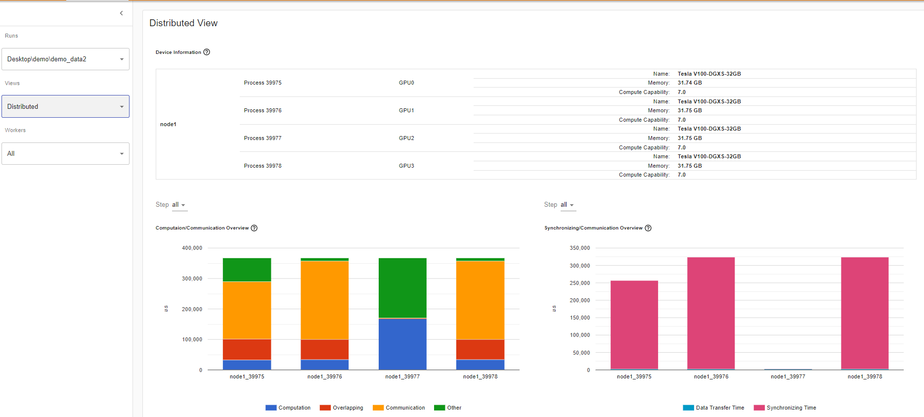
Computation/Communication Overview
In the Computation/Communication overview under the Distributed training view, you can observe the computation-to-communication ratio of each worker and [load balancer](https://en.wikipedia.org/wiki/Load_balancing_(computing) nodes between worker as measured by granularity.
Scenario 1:
If the computation and overlapping time of one worker is much larger than the others, this may suggest an issue in the workload balance or worker being a straggler. Computation is the sum of kernel time on GPU minus the overlapping time. The overlapping time is the time saved by interleaving communications during computation. The more overlapping time represents better parallelism between computation and communication. Ideally the computation and communication completely overlap with each other. Communication is the total communication time minus the overlapping time. The example image below displays how this scenario appears on Tensorboard.
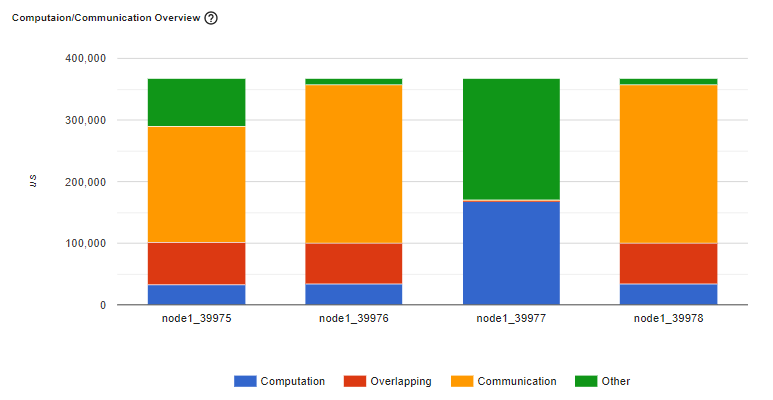
Figure: A straggler example
Scenario 2:
If there is a small batch size (i.e. less computation on each worker) or the data to be transferred is large, the computation-to-communication may also be small and be seen in the profiler with low GPU utilization and long waiting times. This computation/communication view will allow you to diagnose your code to reduce communication by adopting gradient accumulation, or to decrease the communication proportion by increasing batch size. DDP communication time depends on model size. Batch size has no relationship with model size. So increasing batch size could make computation time longer and make computation-to-communication ratio bigger.
Synchronizing/Communication Overview
In the Synchronizing/Communication view, you can observe the efficiency of communication. This is done by taking the step time minus computation and communication time. Synchronizing time is part of the total communication time for waiting and synchronizing with other workers. The Synchronizing/Communication view includes initialization, data loader, CPU computation, and so on Insights like what is the ratio of total communication is really used for exchanging data and what is the idle time of waiting for data from other workers can be drawn from this view.
For example, if there is an inefficient workload balance or straggler issue, you’ll be able to identify it in this Synchronizing/Communication view. This view will show several workers’ waiting time being longer than others.

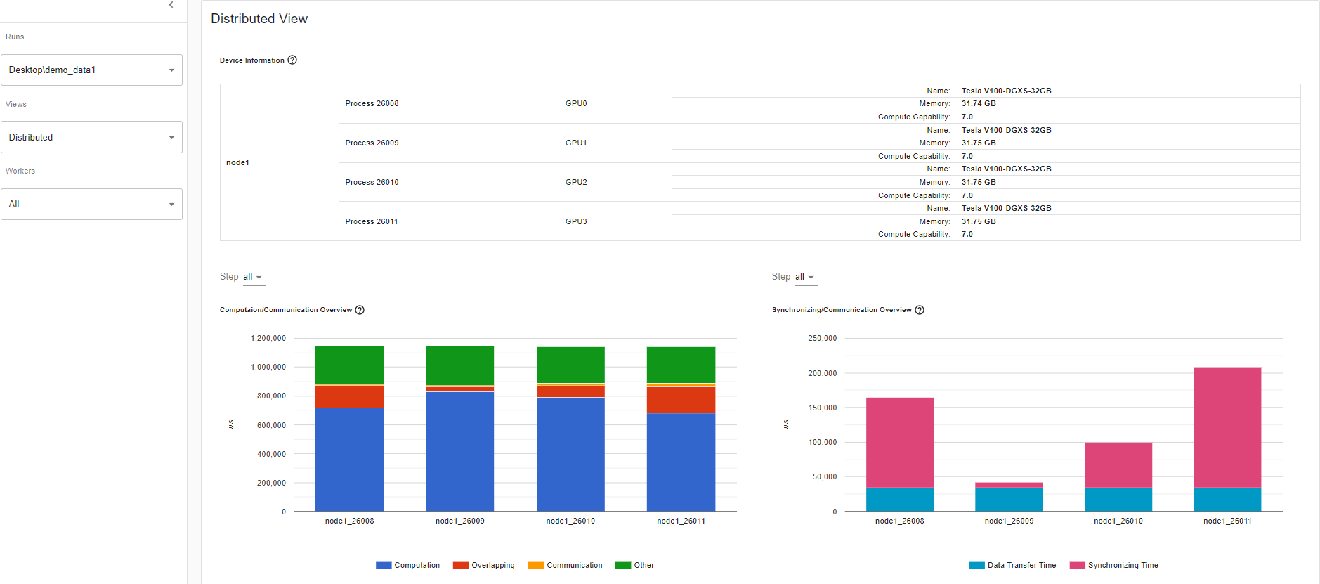
This table view above allows you to see the detailed statistics of all communication ops in each node. This allows you to see what operation types are being called, how many times each op is called, what is the size of the data being transferred by each op, etc.
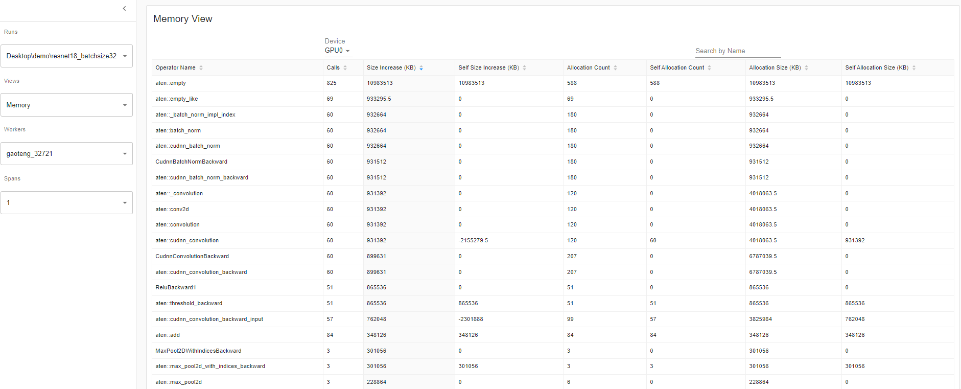
Memory View:
This memory view tool helps you understand the hardware resource consumption of the operators in your model. Understanding the time and memory consumption on the operator-level allows you to resolve performance bottlenecks and in turn, allow your model to execute faster. Given limited GPU memory size, optimizing the memory usage can:
- Allow bigger model which can potentially generalize better on end level tasks.
- Allow bigger batch size. Bigger batch sizes increase the training speed.
The profiler records all the memory allocation during the profiler interval. Selecting the “Device” will allow you to see each operator’s memory usage on the GPU side or host side. You must enable profile_memory=True to generate the below memory data as shown here.
With torch.profiler.profile(
Profiler_memory=True # this will take 1 – 2 minutes to complete.
)
Important Definitions:
• “Size Increase” displays the sum of all allocation bytes and minus all the memory release bytes.
• “Allocation Size” shows the sum of all allocation bytes without considering the memory release.
• “Self” means the allocated memory is not from any child operators, instead by the operator itself.
GPU Metric on Timeline:
This feature will help you debug performance issues when one or more GPU are underutilized. Ideally, your program should have high GPU utilization (aiming for 100% GPU utilization), minimal CPU to GPU communication, and no overhead.
Overview:
The overview page highlights the results of three important GPU usage metrics at different levels (i.e. GPU Utilization, Est. SM Efficiency, and Est. Achieved Occupancy). Essentially, each GPU has a bunch of SM each with a bunch of warps that can execute a bunch of threads concurrently. Warps execute a bunch because the amount depends on the GPU. But at a high level, this GPU Metric on Timeline tool allows you can see the whole stack, which is useful.
If the GPU utilization result is low, this suggests a potential bottleneck is present in your model. Common reasons:
•Insufficient parallelism in kernels (i.e., low batch size)
•Small kernels called in a loop. This is to say the launch overheads are not amortized
•CPU or I/O bottlenecks lead to the GPU not receiving enough work to keep busy
Looking of the overview page where the performance recommendation section is where you’ll find potential suggestions on how to increase that GPU utilization. In this example, GPU utilization is low so the performance recommendation was to increase batch size. Increasing batch size 4 to 32, as per the performance recommendation, increased the GPU Utilization by 60.68%.
GPU Utilization: the step interval time in the profiler when a GPU engine was executing a workload. The high the utilization %, the better. The drawback of using GPU utilization solely to diagnose performance bottlenecks is it is too high-level and coarse. It won’t be able to tell you how many Streaming Multiprocessors are in use. Note that while this metric is useful for detecting periods of idleness, a high value does not indicate efficient use of the GPU, only that it is doing anything at all. For instance, a kernel with a single thread running continuously will get a GPU Utilization of 100%
Estimated Stream Multiprocessor Efficiency (Est. SM Efficiency) is a finer grained metric, it indicates what percentage of SMs are in use at any point in the trace This metric reports the percentage of time where there is at least one active warp on a SM and those that are stalled (NVIDIA doc). Est. SM Efficiency also has it’s limitation. For instance, a kernel with only one thread per block can’t fully use each SM. SM Efficiency does not tell us how busy each SM is, only that they are doing anything at all, which can include stalling while waiting on the result of a memory load. To keep an SM busy, it is necessary to have a sufficient number of ready warps that can be run whenever a stall occurs
Estimated Achieved Occupancy (Est. Achieved Occupancy) is a layer deeper than Est. SM Efficiency and GPU Utilization for diagnosing performance issues. Estimated Achieved Occupancy indicates how many warps can be active at once per SMs. Having a sufficient number of active warps is usually key to achieving good throughput. Unlike GPU Utilization and SM Efficiency, it is not a goal to make this value as high as possible. As a rule of thumb, good throughput gains can be had by improving this metric to 15% and above. But at some point you will hit diminishing returns. If the value is already at 30% for example, further gains will be uncertain. This metric reports the average values of all warp schedulers for the kernel execution period (NVIDIA doc). The larger the Est. Achieve Occupancy value is the better.
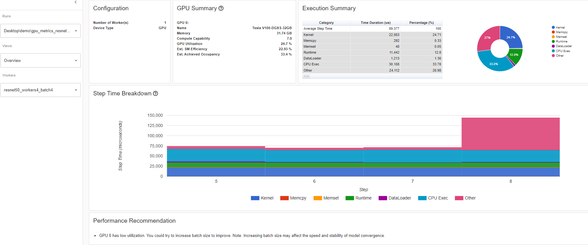
Overview details: Resnet50_batchsize4
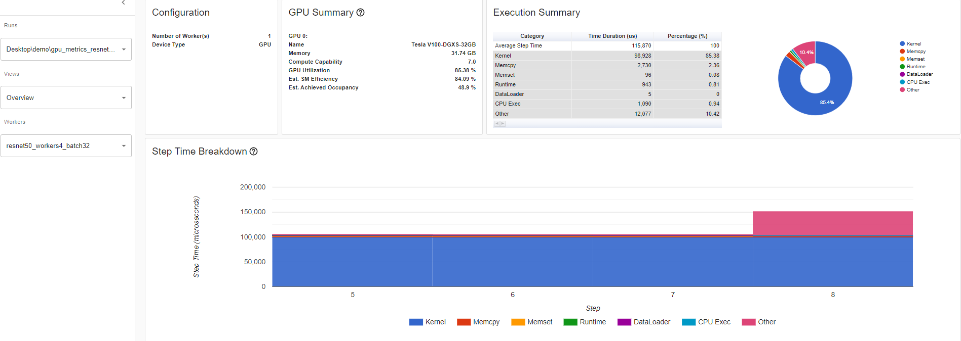
Overview details: Resnet50_batchsize32
Kernel View
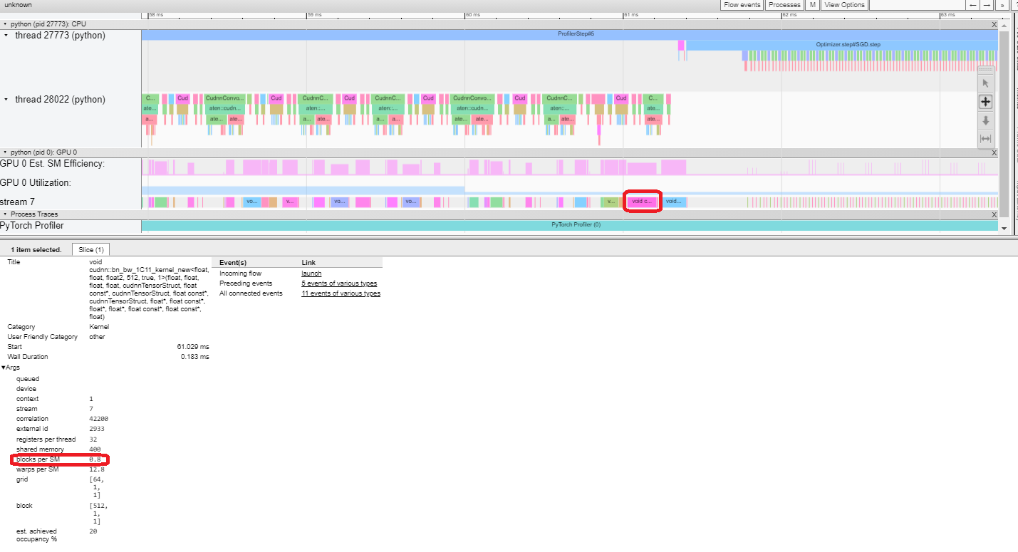
The kernel has “Blocks per SM” and “Est. Achieved Occupancy” which is a great tool to compare model runs.
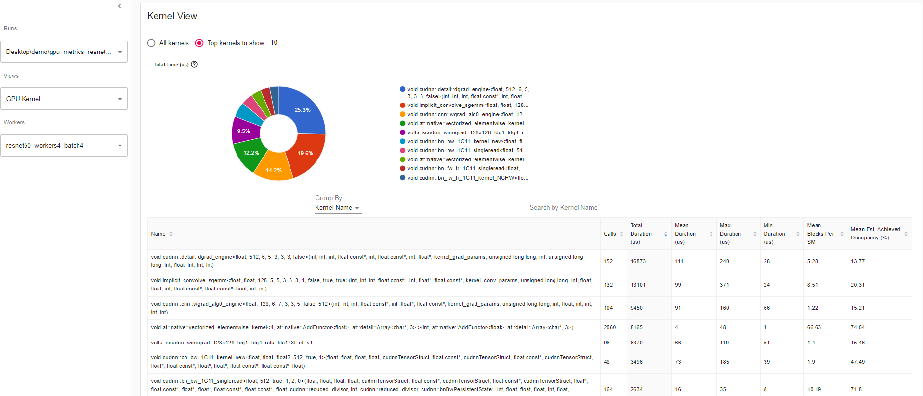
Mean Blocks per SM:
Blocks per SM = Blocks of this kernel / SM number of this GPU. If this number is less than 1, it indicates the GPU multiprocessors are not fully utilized. “Mean Blocks per SM” is weighted average of all runs of this kernel name, using each run’s duration as weight.
Mean Est. Achieved Occupancy:
Est. Achieved Occupancy is defined as above in overview. “Mean Est. Achieved Occupancy” is weighted average of all runs of this kernel name, using each run’s duration as weight.
Trace View
This trace view displays a timeline that shows the duration of operators in your model and which system executed the operation. This view can help you identify whether the high consumption and long execution is because of input or model training. Currently, this trace view shows GPU Utilization and Est. SM Efficiency on a timeline.
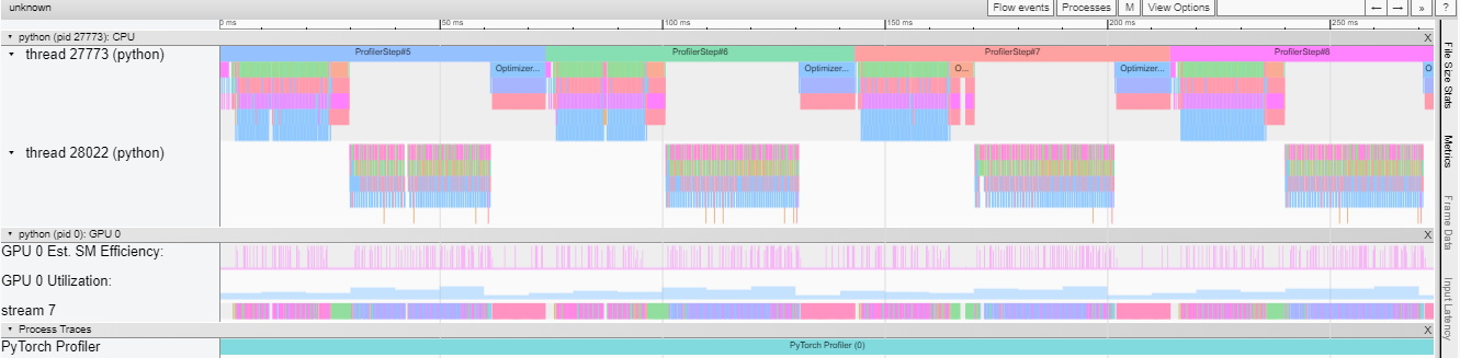
GPU utilization is calculated independently and divided into multiple 10 millisecond buckets. The buckets’ GPU utilization values are drawn alongside the timeline between 0 – 100%. In the above example, the “ProfilerStep5” GPU utilization during thread 28022’s busy time is higher than the following the one during “Optimizer.step”. This is where you can zoom-in to investigate why that is.
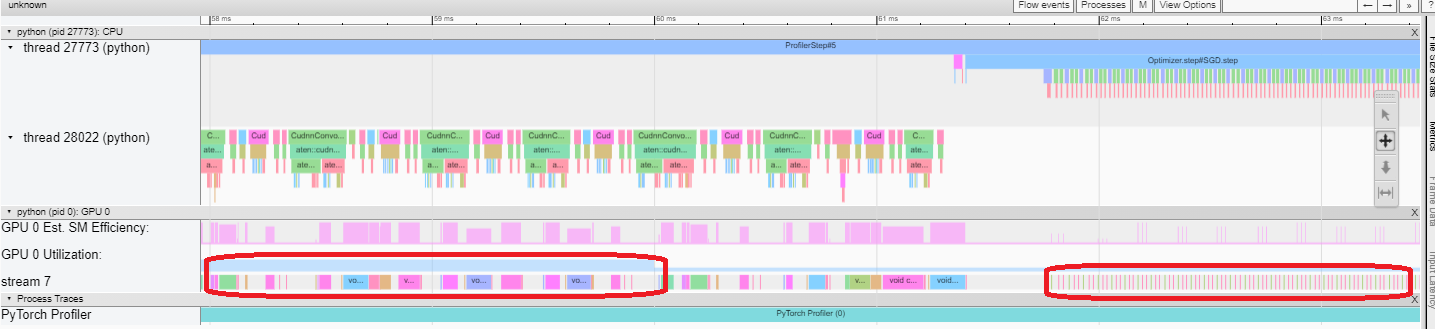
From above, we can see the former’s kernels are longer than the later’s kernels. The later’s kernels are too short in execution, which results in lower GPU utilization.
Est. SM Efficiency: Each kernel has a calculated est. SM efficiency between 0 – 100%. For example, the below kernel has only 64 blocks, while the SMs in this GPU is 80. Then its “Est. SM Efficiency” is 64/80, which is 0.8.
Cloud Storage Support
After running pip install tensorboard, to have data be read through these cloud providers, you can now run:
torch-tb-profiler[blob]
torch-tb-profiler[gs]
torch-tb-profiler[s3]
pip install torch-tb-profiler[blob], pip install torch-tb-profiler[gs], or pip install torch-tb-profiler[S3] to have data be read through these cloud providers. For more information, please refer to this README.
Jump to Source Code:
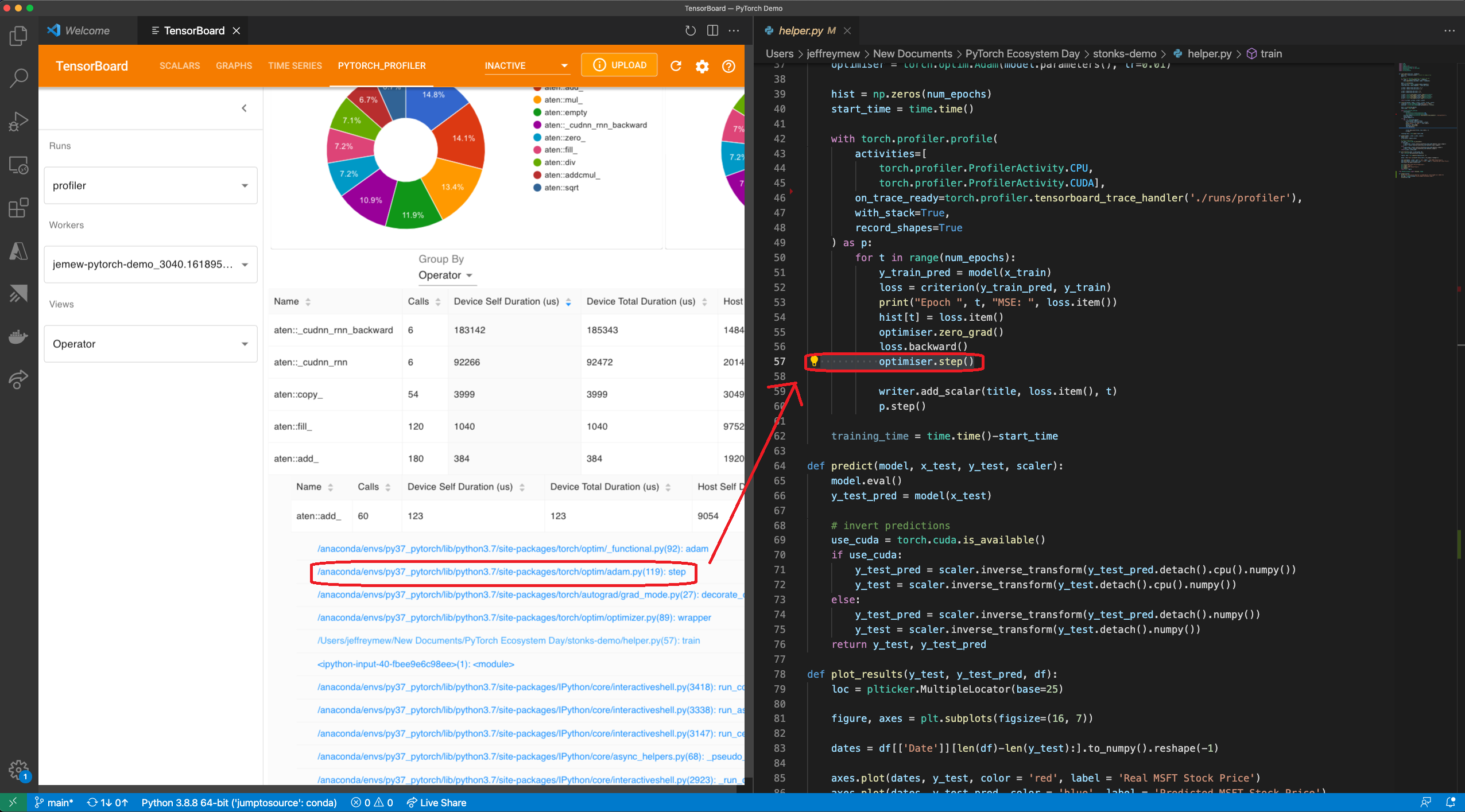
One of the great benefits of having both TensorBoard and the PyTorch Profiler being integrated directly in Visual Studio Code (VS Code) is the ability to directly jump to the source code (file and line) from the profiler stack traces. VS Code Python Extension now supports TensorBoard Integration.
Jump to source is ONLY available when Tensorboard is launched within VS Code. Stack tracing will appear on the plugin UI if the profiling with_stack=True. When you click on a stack trace from the PyTorch Profiler, VS Code will automatically open the corresponding file side by side and jump directly to the line of code of interest for you to debug. This allows you to quickly make actionable optimizations and changes to your code based on the profiling results and suggestions.
Gify: Jump to Source using Visual Studio Code Plug In UI
For how to optimize batch size performance, check out the step-by-step tutorial here. PyTorch Profiler is also integrated with PyTorch Lightning and you can simply launch your lightning training jobs with –trainer.profiler=pytorch flag to generate the traces. Check out an example here.
What’s Next for the PyTorch Profiler?
You just saw how PyTorch Profiler can help optimize a model. You can now try the Profiler by pip install torch-tb-profiler to optimize your PyTorch model.
Look out for an advanced version of this tutorial in the future. If you want tailored enterprise-grade support for this, check out PyTorch Enterprise on Azure. We are also thrilled to continue to bring state-of-the-art tool to PyTorch users to improve ML performance. We’d love to hear from you. Feel free to open an issue here.
For new and exciting features coming up with PyTorch Profiler, follow @PyTorch on Twitter and check us out on pytorch.org.
Building architectures that can handle the world’s data
Most architectures used by AI systems today are specialists. A 2D residual network may be a good choice for processing images, but at best it’s a loose fit for other kinds of data — such as the Lidar signals used in self-driving cars or the torques used in robotics. What’s more, standard architectures are often designed with only one task in mind, often leading engineers to bend over backwards to reshape, distort, or otherwise modify their inputs and outputs in hopes that a standard architecture can learn to handle their problem correctly. Dealing with more than one kind of data, like the sounds and images that make up videos, is even more complicated and usually involves complex, hand-tuned systems built from many different parts, even for simple tasks. As part of DeepMind’s mission of solving intelligence to advance science and humanity, we want to build systems that can solve problems that use many types of inputs and outputs, so we began to explore a more general and versatile architecture that can handle all types of data.Read More
Building architectures that can handle the world’s data
Perceiver IO, a more general version of the Perceiver architecture, can produce a wide variety of outputs from many different inputs.Read More
Simplify and automate anomaly detection in streaming data with Amazon Lookout for Metrics
Do you want to monitor your business metrics and detect anomalies in your existing streaming data pipelines? Amazon Lookout for Metrics is a service that uses machine learning (ML) to detect anomalies in your time series data. The service goes beyond simple anomaly detection. It allows developers to set up autonomous monitoring for important metrics to detect anomalies and identify their root cause in a matter of few clicks, using the same technology used by Amazon internally to detect anomalies in its metrics—all with no ML experience required. However, one limitation you may face if you have an existing Amazon Kinesis Data Streams data pipeline is not being able to directly run anomaly detection on your data streams using Lookout for Metrics. As of this writing, Lookout for Metrics doesn’t have native integration with Kinesis Data Streams to ingest streaming data and run anomaly detection on it.
In this post, we show you how to solve this problem by using an AWS Glue Spark streaming extract, transform, and load (ETL) script to ingest and organize streaming data in Amazon Simple Storage Service (Amazon S3) and using a Lookout for Metrics live detector to detect anomalies. If you have an existing Kinesis Data Streams pipeline that ingests ecommerce data, for example, you can use the solution to detect anomalies such as unexpected dips in revenue, high rates of abandoned shopping carts, increases in new user signups, and many more.
Included in this post is a sample streaming data generator to help you get started quickly. The included GitHub repo provides step-by-step deployment instructions, and uses the AWS Cloud Development Kit (AWS CDK) to simplify and automate the deployment.
Lookout for Metrics allows users to set up anomaly detectors in both continuous and backtest modes. Backtesting allows you to detect anomalies on historical data. This feature is helpful when you want to try out the service on past data or validate against known anomalies that occurred in the past. For this post, we use continuous mode, where you can detect anomalies on live data as they occur. In continuous mode, the detector monitors an input S3 bucket for continuous data and runs anomaly detection on new data at specified time intervals. For the live detector to consume continuous time series data from Amazon S3 correctly, it needs to know where to look for data for the current time interval, therefore, it requires continuous input data in S3 buckets organized by time interval.
Overview of solution
The solution architecture consists of the following components:
- Streaming data generator – To help you get started quickly, we provide Python code that generates sample time series data and writes to a Kinesis data stream at a specified time interval. The provided code generates sample data for an ecommerce schema (
platform,marketplace,event_time,views,revenue). You can also use your own data stream and data, but you must update the downstream processes in the architecture to process your schema. - Kinesis Data Streams to Lookout for Metrics – The AWS Glue Spark streaming ETL code is the core component of the solution. It contains logic to do the following:
- Ingest streaming data
- Micro-batch data by time interval
- Filter dimensions and metrics columns
- Deliver filtered data to Amazon S3 grouped by timestamp
- Lookout for Metrics continuous detector – The AWS Glue streaming ETL code writes time series data as CSV files to the S3 bucket, with objects organized by time interval. The Lookout for Metrics continuous detector monitors the S3 bucket for live data and runs anomaly detection at the specified time interval (for example, every 5 minutes). You can view the detected anomalies on the Lookout for Metrics dashboard.
The following diagram illustrates the solution architecture.

AWS Glue Spark streaming ETL script
The main component of the solution is the AWS Glue serverless streaming ETL script. The script contains the logic to ingest the streaming data and write the output, grouped by time interval, to an S3 bucket. This makes it possible for Lookout for Metrics to use streaming data from Kinesis Data Streams to detect anomalies. In this section, we walk through the Spark streaming ETL script used by AWS Glue.
The AWS Glue Spark streaming ETL script performs the following steps:
- Read from the AWS Glue table that uses Kinesis Data Streams as the data source.
The following screenshot shows the AWS Glue table created for the ecommerce data schema.

- Ingest the streaming data from the AWS Glue table (
table_nameparameter) batched by time window (stream_batch_timeparameter) and create a data frame for each micro-batch usingcreate_data_frame.from_catalog(), as shown in the following code:
data_frame_datasource0 = glueContext.create_data_frame.from_catalog(stream_batch_time = BATCH_WIN_SIZE,
                            database = glue_dbname, table_name = glue_tablename, transformation_ctx = "datasource0",
additional_options = {"startingPosition": "TRIM_HORIZON", "inferSchema": "false"})- Perform the following processing steps for each batch of data (data frame) ingested:
- Select only the required columns and convert the data frame to the AWS Glue native DynamicFrame.
datasource0 = DynamicFrame.fromDF(data_frame, glueContext, "from_data_frame").select_fields(['marketplace','event_time', 'views'])As shown in the preceding example code, select only the columns marketplace, event_time, and views to write to output CSV files in Amazon S3. Lookout for Metrics uses these columns for running anomaly detection. In this example, marketplace is the optional dimension column used for grouping anomalies, views is the metric to be monitored for anomalies, and event_time is the timestamp for time series data.
-
- Populate the time interval in each streaming record ingested:
datasource1 = Map.apply(frame=datasource0, f=populateTimeInterval)In the preceding code, we provide the custom function populateTimeInterval, which determines the appropriate time interval for the given data point based on its event_time timestamp column.
The following table includes example time intervals determined by the function for a 5-minute frequency.
| Input timestamp | Start of time interval determined by populateTimeInterval function |
| 2021-05-24 19:18:28 | 2021-05-24 19:15 |
| 2021-05-24 19:21:15 | 2021-05-24 19:20 |
The following table includes example time intervals determined by the function for a 10-minute frequency.
| Input timestamp | Start of time interval determined by populateTimeInterval function |
| 2021-05-24 19:18:28 | 2021-05-24 19:10 |
| 2021-05-24 19:21:15 | 2021-05-24 19:20 |
-
- The
write_dynamic_frame() function uses the time interval (as determined in the previous step) as the partition key to write output CSV files to the appropriate S3 prefix structure:
- The
datasink1 = glueContext.write_dynamic_frame.from_options(frame = datasource1, connection_type = "s3",
                        connection_options = {"path": path_datasink1, "partitionKeys": ["intvl_date", "intvl_hhmm"]},
                        format_options={"quoteChar": -1, "timestamp.formats": "yyyy-MM-dd HH:mm:ss"},
                        format = src_format, transformation_ctx = "datasink1")
For example, the following screenshot shows that the ETL script writes output to the S3 folder structure organized by 5-minute time intervals.
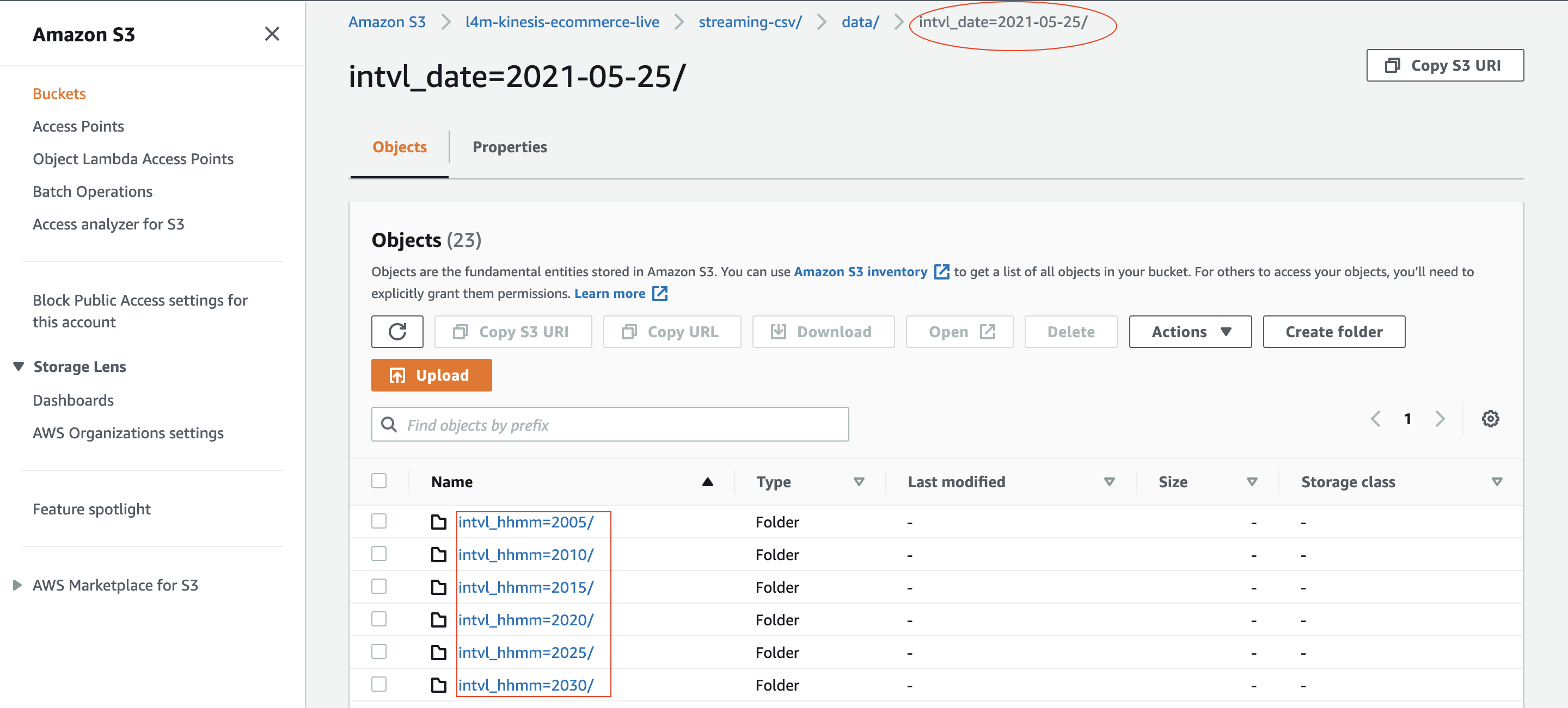
For additional details on partitions for ETL outputs, see Managing Partitions for ETL Output in AWS Glue.
You can set up a live detector using Amazon S3 as a continuous data source to start detecting the anomalies in streaming data. For detailed instructions, see GitHub repo.
Prerequisites
You need the following to deploy the solution:
- An AWS account with permissions to deploy the solution using AWS CDK
- A workstation or development environment with the following installed and configured:
- npm
- Typescript
- AWS CDK
- AWS account credentials
You can find detailed instructions in the “Getting Started” section of the GitHub repo.
Deploy the solution
Follow the step-by-step instructions in the GitHub repo to deploy the solution components. AWS CDK templates are provided for each of the solution components, organized in their own directory structure within the GitHub repo. The templates deploy the following resources:
- Data generator – The Lambda function, Amazon EventBridge rule, and Kinesis data stream
- Connector for Lookout for Metrics – The AWS Glue Spark streaming ETL job and S3 bucket
- Lookout for Metrics continuous detector – Our continuous detector
Clean up
To avoid incurring future charges, delete the resources by deleting the stacks deployed by the AWS CDK.
Conclusion
In this post, we showed how you can detect anomalies in streaming data sources using a Lookout for Metrics continuous detector. The solution used serverless streaming ETL with AWS Glue to prepare the data for Lookout for Metrics anomaly detection. The reference implementation used an ecommerce sample data schema (platform, marketplace, event_time, views, revenue) to demonstrate and test the solution.
You can easily extend the provided data generator code and ETL script to process your own schema and sample data. Additionally, you can adjust the solution parameters such as anomaly detection frequency to match your use case. With minor changes, you can replace the sample data generator with an existing Kinesis Data Streams streaming data source.
To learn more about Amazon Lookout for Metrics, see Introducing Amazon Lookout for Metrics: An anomaly detection service to proactively monitor the health of your business and the Lookout for Metrics Developer Guide. For additional information about streaming ETL jobs with AWS Glue, see Crafting serverless streaming ETL jobs with AWS Glue and Adding Streaming ETL Jobs in AWS Glue.
About the Author
 Babu Srinivasan is a Sr. Solutions Architect at AWS, with over 24 years of experience in IT and the last 6 years focused on the AWS Cloud. He is passionate about AI/ML. Outside of work, he enjoys woodworking and entertains friends and family (sometimes strangers) with sleight of hand card magic.
Google at ACL 2021
Posted by Catherine Armato, Program Manager
This week, the 59th annual meeting of the Association for Computational Linguistics (ACL), a premier conference covering a broad spectrum of research areas that are concerned with computational approaches to natural language, is taking place online.
As a leader in natural language processing and understanding, and a Diamond Level sponsor of ACL 2021, Google will showcase the latest research in the field with over 35 publications, and the organization of and participation in a variety of workshops and tutorials.
If you’re registered for ACL 2021, we hope that you’ll visit the Google virtual booth in Gather Town to learn more about the projects and opportunities at Google that go into solving interesting problems for billions of people. You can also learn more about Google’s participation on the ACL 2021 Expo page, and see a full list of Google publications below (Google affiliations in bold).
Organizing Committee
Senior Area Chairs include: Dan Roth, Emily Pitler, Jimmy Lin, Ming-Wei Chang, Sebastian Ruder, Slav Petrov
Area Chairs include: Ankur P. Parikh, Artem Sokolov, Bhuwan Dhingra, Cicero Nogueira dos Santos, Colin Cherry, Dani Yogatama, David Mimno, Hideto Kazawa, Ian Tenney, Jasmijn Bastings, Jun Suzuki, Katja Filippova, Kyle Gorma, Lu Wang, Manaal Faruqui, Natalie Schluter, Peter Liu, Radu Soricut, Sebastian Gehrmann, Shashi Narayan, Tal Linzen, Vinodkumar Prabhakaran, Waleed Ammar
Publications
Parameter-Efficient Multi-task Fine-Tuning for Transformers via Shared Hypernetwork
Rabeeh Karimi Mahabadi*, Sebastian Ruder, Mostafa Dehghani, James Henderson
TicketTalk: Toward Human-Level Performance with End-to-End, Transaction-Based Dialog Systems
Bill Byrne, Karthik Krishnamoorthi, Saravanan Ganesh, Mihir Sanjay Kale
Increasing Faithfulness in Knowledge-Grounded Dialogue with Controllable Feature
Hannah Rashkin, David Reitter, Gaurav Singh Tomar, Dipanjan Das
Compositional Generalization and Natural Language Variation: Can a Semantic Parsing Approach Handle Both?
Peter Shaw, Ming-Wei Chang, Panupong Pasupat, Kristina Toutanova
Exploiting Language Relatedness for Low Web-Resource Language Model Adaptation: An Indic Languages Study
Yash Khemchandani, Sarvesh Mehtani, Vaidehi Patil, Abhijeet Awasthi, Partha Talukdar, Sunita Sarawagi
Causal Analysis of Syntactic Agreement Mechanisms in Neural Language Model
Matthew Finlayson, Aaron Mueller, Sebastian Gehrmann, Stuart Shieber, Tal Linzen*, Yonatan Belinkov
Modeling Fine-Grained Entity Types with Box Embeddings
Yasumasa Onoe, Michael Boratko, Andrew McCallum, Greg Durrett
TextSETTR: Few-Shot Text Style Extraction and Tunable Targeted Restyling
Parker Riley*, Noah Constant, Mandy Guo, Girish Kumar*, David Uthus, Zarana Parekh
Which Linguist Invented the Lightbulb? Presupposition Verification for Question-Answering
Najoung Kim*, Ellie Pavlick, Burcu Karagol Ayan, Deepak Ramachandran
H-Transformer-1D: Fast One-Dimensional Hierarchical Attention for Sequences
Zhenhai Zhu, Radu Soricut
Are Pretrained Convolutions Better than Pretrained Transformers?
Yi Tay, Mostafa Dehghani, Jai Gupta, Dara Bahri, Vamsi Aribandi, Zhen Qin, Donald Metzler
Benchmarking Scalable Methods for Streaming Cross Document Entity Coreference
Robert L Logan IV, Andrew McCallum, Sameer Singh, Dan Bikel
PhotoChat: A Human-Human Dialogue Dataset With Photo Sharing Behavior For Joint Image-Text Modeling
Xiaoxue Zang, Lijuan Liu, Maria Wang, Yang Song*, Hao Zhang, Jindong Chen
Focus Attention: Promoting Faithfulness and Diversity in Summarization
Rahul Aralikatte*, Shashi Narayan, Joshua Maynez, Sascha Rothe, Ryan McDonald*
A Cognitive Regularizer for Language Modeling
Jason Wei, Clara Meister, Ryan Cotterell
Language Model Augmented Relevance Score
Ruibo Liu, Jason Wei, Soroush Vosoughi
Cross-Replication Reliability – An Empirical Approach to Interpreting Inter-rater Reliability
Ka Wong, Praveen Paritosh, Lora Aroyo
TIMEDIAL: Temporal Commonsense Reasoning in Dialog
Lianhui Qin*, Aditya Gupta, Shyam Upadhyay, Luheng He, Yejin Choi, Manaal Faruqui
StructFormer: Joint Unsupervised Induction of Dependency and Constituency Structure from Masked Language Modeling
Yikang Shen*, Yi Tay, Che Zheng, Dara Bahri, Donald Metzler, Aaron Courville
MOLEMAN: Mention-Only Linking of Entities with a Mention Annotation Network
Nicholas FitzGerald, Jan A. Botha, Daniel Gillick, Daniel M. Bikel, Tom Kwiatkowski, Andrew McCallum
Neural Retrieval for Question Answering with Cross-Attention Supervised Data Augmentation
Yinfei Yanga, Ning Jinb, Kuo Linb, Mandy Guoa, Daniel Cera
ROPE: Reading Order Equivariant Positional Encoding for Graph-Based Document Information Extraction
Chen-Yu Lee, Chun-Liang Li, Chu Wang∗, Renshen Wang, Yasuhisa Fujii, Siyang Qin, Ashok Popat, Tomas Pfister
Measuring and Improving BERT’s Mathematical Abilities by Predicting the Order of Reasoning
Piotr Piekos, Henryk Michalewski, Mateusz Malinowsk
Improving Compositional Generalization in Classification Tasks via Structure Annotations
Juyong Kim, Pradeep Ravikumar, Joshua Ainslie, Santiago Ontañón
A Simple Recipe for Multilingual Grammatical Error Correction
Sascha Rothe, Jonathan Mallinson, Eric Malmi, Sebastian Krause, Aliaksei Severyn
nmT5 – Is Parallel Data Still Relevant for Pre-training Massively Multilingual Language Models?
Mihir Kale, Aditya Siddhant, Noah Constant, Melvin Johnson, Rami Al-Rfou, Linting Xue
QA-Driven Zero-Shot Slot Filling with Weak Supervision Pretraining
Xinya Du*, Luheng He, Qi Li, Dian Yu*, Panupong Pasupat, Yuan Zhang
AgreeSum: Agreement-Oriented Multi-Document Summarization
Richard Yuanzhe Pang*, Adam D. Lelkes, Vinh Q. Tran, Cong Yu
Disfl-QA: A Benchmark Dataset for Understanding Disfluencies in Question Answering
Aditya Gupta, Jiacheng Xu*, Shyam Upadhyay, Diyi Yang, Manaal Faruqui
Training ELECTRA Augmented with Multi-word Selection
Jiaming Shen*, Jialu Liu, Tianqi Liu, Cong Yu, Jiawei Han
A Survey of Data Augmentation Approaches for NLP
Steven Y. Feng, Varun Gangal, Jason Wei, Sarath Chandar, Soroush Vosoughi, Teruko Mitamura, Eduard Hovy
RealFormer: Transformer Likes Residual Attention
Ruining He, Anirudh Ravula, Bhargav Kanagal, Joshua Ainslie
Scaling Within Document Coreference to Long Texts
Raghuveer Thirukovalluru, Nicholas Monath, Kumar Shridhar, Manzil Zaheer, Mrinmaya Sachan, Andrew McCallum
MergeDistill: Merging Language Models using Pre-trained Distillation
Simran Khanuja, Melvin Johnson, Partha Talukdar
DoT: An Efficient Double Transformer for NLP tasks with Tables
Syrine Krichene, Thomas Müller*, Julian Martin Eisenschlos
How Reliable are Model Diagnostics?
Vamsi Aribandi, Yi Tay, Donald Metzler
Workshops
Interactive Learning for Natural Language Processing
Organizers include: Filip Radlinski
Invited Panelist: Julia Kreutzer
6th Workshop on Representation Learning for NLP (RepL4NLP-2021)
Organizers include: Chris Dyer, Laura Rimell
Third Workshop on Gender Bias for Natural Language Processing
Organizers include: Kellie Webster
Benchmarking: Past, Present and Future
Invited Speaker: Eunsol Choi
SemEval-2021, 15th International Workshop on Semantic Evaluation
Organizers include: Natalie Schluter
Workshop on Online Abuse and Harms
Organizers include: Vinodkumar Prabhakaran
GEM: Natural Language Generation, Evaluation, and Metrics
Organizers include: Sebastian Gehrmann
Workshop on Natural Language Processing for Programming
Invited Speaker: Charles Sutton
WPT 2021: The 17th International Conference on Parsing Technologies
Organizers include: Weiwei Sun
Tutorial
Recognizing Multimodal Entailment
Instructors include: Cesar Ilharco, Vaiva Imbrasaite, Ricardo Marino, Jannis Bulian, Chen Sun, Afsaneh Shirazi, Lucas Smaira, Cordelia Schmid
* Work conducted while at Google.

Display systems research: Reverse passthrough VR
As AR and VR devices become a bigger part of how we work and play, how do we maintain seamless social connection between real and virtual worlds? In other words, how do we maintain “social co-presence” in shared spaces among people who may or may not be involved in the same AR/VR experience?
This year at SIGGRAPH, Facebook Reality Labs (FRL) Research will present a new concept for social co-presence with virtual reality headsets: reverse passthrough VR, led by research scientist Nathan Matsuda. Put simply, reverse passthrough is an experimental VR research demo that allows the eyes of someone wearing a headset to be seen by the outside world. This is in contrast to what Quest headsets can do today with Passthrough+ and the experimental Passthrough API, which use externally facing cameras to help users easily see their external surroundings while they’re wearing the headset.
Over the years, we’ve made strides in enabling Passthrough features for Oculus for consumers and developers to explore. In fact, the idea for this experimental reverse passthrough research occurred to Matsuda after he spent a day in the office wearing a Quest headset with Passthrough, thinking through how to make mixed reality environments more seamless for social and professional settings. Wearing the headset with Passthrough, he could see his colleagues and the room around him just fine. But his colleagues couldn’t see him without an external display. Every time he attempted to speak to someone, they remarked how strange it was that he wasn’t able to make eye contact. So Matsuda posed the question: What if you could see his eyes — would that add something to the social dynamic?
When Matsuda first demonstrated reverse passthrough for FRL Chief Scientist Michael Abrash in 2019, Abrash was unconvinced about the utility of this work. In the demo, Matsuda wore a custom-built Rift S headset with a 3D display mounted to the front. On the screen, a floating 3D image of Matsuda’s face, crudely rendered from a game engine, re-created his eye gaze using signals from a pair of eye-tracking cameras inside the headset.

Research scientist Nathan Matsuda wears an early reverse passthrough prototype with 2D outward-facing displays. Right: The first fully functional reverse passthrough demo using 3D light field displays.
“My first reaction was that it was kind of a goofy idea, a novelty at best,” said Abrash. “But I don’t tell researchers what to do, because you don’t get innovation without freedom to try new things, and that’s a good thing, because now it’s clearly a unique idea with genuine promise.”
Nearly two years after the initial demo, the 3D display technology and research prototype have evolved significantly, featuring purpose-built optics, electronics, software, and a range of supporting technologies to capture and depict more realistic 3D faces. This progress is promising, but this research is clearly still experimental: Tethered by many cables, it’s far from a standalone headset, and the eye and facial renderings are not yet completely lifelike. However, it is a research prototype designed in the spirit of FRL Research’s core ethos to run with far-flung concepts that may seem a bit outlandish. While this work is nowhere near a product roadmap, it does offer a glimpse into how reverse passthrough could be used in collaborative spaces of the future — both real and virtual.
Left: A VR headset with the external display disabled, representing the current state of the art. No gaze cues are visible through the opaque headset enclosure. Middle: A VR headset with outward-facing 2D displays, as proposed in prior academic works[1][2][3][4]. Some gaze cues are visible, but the incorrect perspective limits the viewer’s ability to discern gaze direction. Right: Our recent prototype uses 3D reverse passthrough displays, showing correct perspective for multiple external viewers.
Reverse passthrough
The essential component in a reverse passthrough headset is the externally facing 3D display. You could simply put a 2D display on the front of the headset and show a flat projection of the user’s face on it, but the offset from the user’s actual face to the front of the headset makes for a visually jarring, unnatural effect that breaks any hope of reading correct eye contact. As the research prototype evolved, it was clear that a 3D display was a better direction, as it would allow the user’s eyes and face to appear at the correct position in space on the front of the headset. This depiction helps maintain alignment as external viewers move in relation to the 3D display.
There are several established ways to display 3D images. For this research, we used a microlens-array light field display because it’s thin, simple to construct, and based on existing consumer LCD technology. These displays use a tiny grid of lenses that send light from different LCD pixels out in different directions, with the effect that an observer sees a different image when looking at the display from different directions. The perspective of the images shift naturally so that any number of people in the room can look at the light field display and see the correct perspective for their location.
As with any early stage research prototype, this hardware still carries significant limitations: First, the viewing angle can’t be too severe, and second, the prototype can only show objects in sharp focus that are within a few centimeters of the physical screen surface. Conversations take place face-to-face, which naturally limits reverse passthrough viewing angles. And the wearer’s face is only a few centimeters from the physical screen surface, so the technology works well for this case — and will work even better if VR headsets continue to shrink in size, using methods such as holographic optics.
Building the research prototype
FRL researchers used a Rift S for early explorations of reverse passthrough. As the concept evolved, the team began iterating on Half Dome 2 to build the research prototype presented this year at SIGGRAPH. Stripping down the headset to the bare display pod, mechanical research engineer Joel Hegland provided a roughly 50-millimeter-thick VR headset to serve as a base for the latest reverse passthrough demo. Then, optical scientist Brian Wheelwright designed a microlens array to be fitted in front.
The resulting headset contains two display pods that are mirror images of each other. They contain an LCD panel and lens for the base VR display. A ring of infrared LEDs illuminates the part of the face covered by the pod. A mirror that is reflective only for infrared light sits between the lens and screen, so that a pair of infrared cameras can view the eye from nearly head-on. Doing all this in the invisible infrared band keeps the eye imaging system from distracting the user from the VR display itself. Then the front of the pod has another LCD with the microlens array.


Left: A cutaway view of one of the prototype display pods. Right: The prototype display pod with driver electronics, prior to installation in the full headset prototype.
Imaging eyes and faces in 3D
Producing the interleaved 3D images to show on the light field display presented a significant challenge in itself. For this research prototype, Matsuda and team opted to use a stereo camera pair to produce a surface model of the face, then projected the views of the eye onto that surface. While the resulting projected eyes and face are not lifelike, this is just a short-term solution to pave the way for future development.
FRL’s Codec Avatars research points toward the next generation of this imaging. Codec Avatars are realistic representations of the human face, expressions, voice, and body that, via deep learning, can be driven from a compact set of measurements taken inside a VR headset in real time. These virtual avatars should be much more effective for reverse passthrough, allowing for a unified system of facial representation that works whether the viewer is local or remote.
Shown below, a short video depicts a Codec Avatar from our Pittsburgh lab running on the prototype reverse passthrough headset. These images, and their motion over time, appear much more lifelike than those captured using the current stereo camera method, indicating the sort of improvements that such a system could provide while working in tandem with remote telepresence systems.
The reverse passthrough prototype displaying a high-fidelity Codec Avatar facial reconstruction.
A path toward social co-presence in VR
Totally immersive VR and AR glasses with a display are fundamentally different technologies that will likely end up serving different users in different scenarios in the long term. There will be situations where people will need the true transparent optics of AR glasses, and others where people will prefer the image quality and immersion of VR. Facebook Reality Labs Research, under Michael Abrash’s direction, has cast a wide net when probing new technical concepts in order to move the ball forward across both of these display architectures. Fully exploring this space will ensure that the lab has a grasp on the full range of possibilities — and limitations — for future AR/VR devices, and eventually put those findings into practice in a way that supports human-computer interaction for the most people in the most places.
Reverse passthrough is representative of this sort of work — an example of how ideas from around the lab are pushing the utility of VR headsets forward. Later this year, we’ll give a more holistic update on our display systems research and show how all this work — from varifocal, holographic optics, eye tracking, and distortion correction to reverse passthrough — is coming together to help us pass what we call the Visual Turing Test in VR.
Ultimately, these innovations and more will come together to create VR headsets that are compact, light, and all-day wearable; that mix high-quality virtual images with high-quality real-world images; and that let you be socially present with anyone in the world, whether they’re on the other side of the planet or standing next to you. Making that happen is our goal at Facebook Reality Labs Research.
[1] Liwei Chan and Kouta Minamizawa. 2017. FrontFace: Facilitating Communication between HMD Users and Outsiders Using Front-Facing-Screen HMDs
[2] Kana Misawa and Jun Rekimoto. 2015. ChameleonMask: Embodied Physical and Social Telepresence using Human Surrogates
[3] Christian Mai, Lukas Rambold, and Mohamed Khamis. 2017. TransparentHMD: Revealing the HMD User’s Face to Bystanders
[4] Jan Gugenheimer, Christian Mai, Mark McGill, Julie Williamson, Frank Steinicke, and Ken Perlin. 2019. Challenges Using Head-Mounted Displays in Shared and Social SpacesThe post Display systems research: Reverse passthrough VR appeared first on Facebook Research.
Better Than 8K Resolution: NVIDIA Inception Displays Global AI Startup Ecosystem
There are more AI startups in healthcare than any other single industry. The number of AI startups in media and entertainment is about the same as that in retail. More than one in 10 of all AI startups is based in California.
How do we know this? NVIDIA Inception, our acceleration platform for AI startups, has now surpassed 8,500 members. That’s about two-thirds of the total number of AI startups worldwide, as estimated by Pitchbook. With total cumulative funding of over $60 billion and members in 90 countries, NVIDIA Inception is one of the largest AI startup ecosystems in the world.
With this type of scale, NVIDIA Inception is more than a singular program; it’s a reflection of the larger startup landscape. And there’s plenty that can be inferred based on this.
Data Across 8,500+ Startups
NVIDIA Inception figures show the United States leads the world in terms of both the number of AI startups, representing nearly 27 percent, and the amount of secured funding, accounting for over $27 billion in cumulative funding.
Of U.S.-based startups, 42 percent were based in California — more than one in 10 AI startups is based in the state — with 29 percent in the San Francisco Bay Area. This underscores the continued draw of the region for startup founders and VC funding.
Following the U.S. is China, in terms of both funding and company stage, with 12 percent of NVIDIA Inception members based there. India comes in third at 7 percent, with the United Kingdom right behind at 6 percent.
Taken together, AI startups based in the U.S., China, India and the U.K. account for just over half of all startups in NVIDIA Inception. Following in order after these are Germany, Russia, France, Sweden, Netherlands, Korea and Japan.
In terms of industries, healthcare, IT services, intelligent video analytics (IVA), media and entertainment (M&E) and robotics are the top five in NVIDIA Inception. AI startups in healthcare account for 16 percent of Inception members, followed by those in IT services at 15 percent. AI startups in IVA make up 8 percent, with M&E and robotics AI startups tied at 7 percent.
Details Spanning 3,000+ Startups Since 2020
More than 3,000 AI startups have joined NVIDIA Inception since 2020. Similar to data across Inception as a whole, AI startups from the U.S. account for the largest segment (27 percent), followed by China (12 percent), and India and the U.K. (tied at 6 percent).
Additionally, startups that have joined since 2020 are concentrated in the same top five industries, though in slightly different order. IT services leads the way at 17 percent, followed by healthcare at 16 percent, M&E at 9 percent, IVA at 8 percent and robotics at 5 percent.
Within the top two industries — healthcare and IT services — there’s more detail among AI startups who have joined since 2020. The dominant segment within IT services is computer vision at 27 percent, with predictive analytics in second place at 9 percent. The top two segments in healthcare are medical analytics at 38 percent and medical imaging at 36 percent, though the fastest growth is among AI startups in the pharma and AI biology industries at 15 percent.
Virtual and augmented reality startup companies are far outpacing any other segment within M&E, mostly due to the pandemic. These startups are coming to NVIDIA Inception with a shared vision of building an ecosystem for the metaverse.
Disruption Through Startups
Since Inception’s launch in 2016, it has grown more than tenfold. This growth has accelerated year over year, with membership increasing to 26 percent in 2020, and already reaching 17 percent in the first half of 2021.
NVIDIA Inception is a program built to accommodate and nurture every startup that is accelerating computing, at every stage in their journey. All program benefits are free of charge — there are no fees ever. And unlike other accelerators or incubators, startups never have to give up equity to join.
Startups are the single best lens into the future of modern AI, so join with us today by applying for NVIDIA Inception.
The post Better Than 8K Resolution: NVIDIA Inception Displays Global AI Startup Ecosystem appeared first on The Official NVIDIA Blog.
Eugene Yan and the art of writing about science
Why the Amazon applied scientist takes the time to break down his work for readers.Read More
Stanford AI Lab Papers at ACL-IJCNLP 2021
![]()
The Joint Conference of the 59th Annual Meeting of the Association for Computational Linguistics and the 11th
International Joint Conference on Natural Language Processing
is being hosted virtually this week. We’re excited to share all the work from SAIL that’s being presented, and you’ll find links to papers, videos and blogs below. Feel free to reach out to the contact authors directly to learn more about the work that’s happening at Stanford!
List of Accepted Long Papers
Neural Event Semantics for Grounded Language Understanding

Authors: Shyamal Buch, Li Fei-Fei, Noah D. Goodman
Contact: shyamal@cs.stanford.edu
Links: Paper | Project Webpage
Keywords: grounded language, compositionality, modular networks, event semantics
Notes: Accepted as a paper to TACL 2021, presented at ACL-IJCNLP 2021!
Measuring Conversational Update: A Case Study on Student-Teacher Interactions
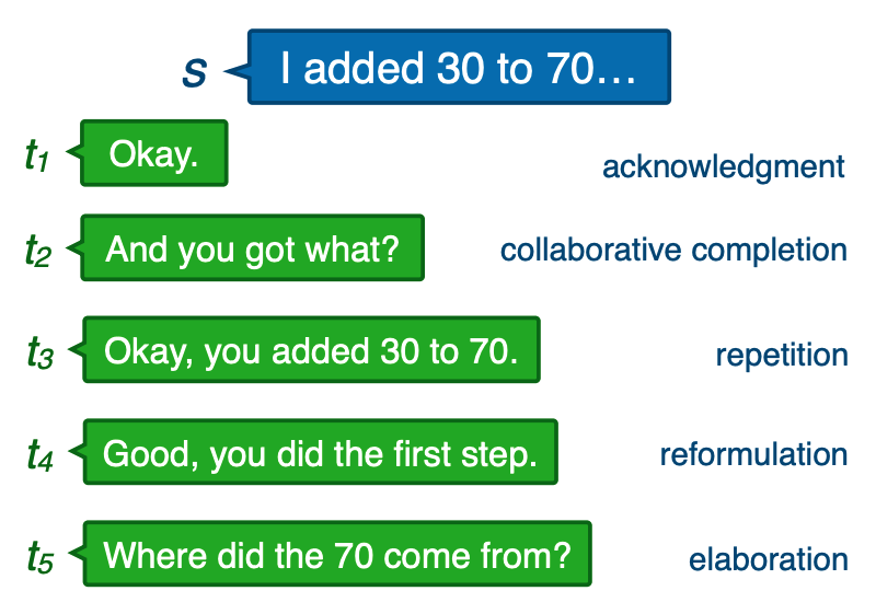
Authors: Dorottya Demszky, Jing Liu, Zid Mancenido, Julie Cohen, Heather Hill, Dan Jurafsky, Tatsunori Hashimoto
Contact: ddemszky@stanford.edu
Links: Paper | Code & Data
Keywords: conversational uptake, education
Mind Your Outliers! Investigating the Negative Impact of Outliers on Active Learning for Visual Question Answering
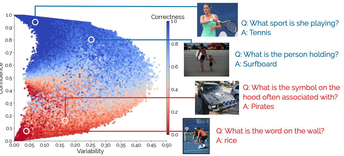
Authors: Siddharth Karamcheti, Ranjay Krishna, Li Fei-Fei, Christopher D. Manning
Contact: skaramcheti@cs.stanford.edu
Links: Paper | Code
Keywords: active learning, visual question answering, interpretability
Notes: Outstanding Paper Award
Relevance-guided Supervision for OpenQA with ColBERT

Authors: Omar Khattab, Christopher Potts, Matei Zaharia
Contact: okhattab@stanford.edu
Links: Paper | Code
Keywords: open-domain question answering, neural retrieval, weak supervision
Notes: Accepted as a paper to TACL 2021, presented at ACL-IJCNLP 2021!
Prefix Tuning: Optimizing Continuous Prompts for Generation

Authors: Xiang Lisa Li, Percy Liang
Contact: xlisali@stanford.edu
Links: Paper | Code
Keywords: prefix-tuning, fine-tuning for generation, large-scale fine-tuning
DynaSent: A Dynamic Benchmark for Sentiment Analysis
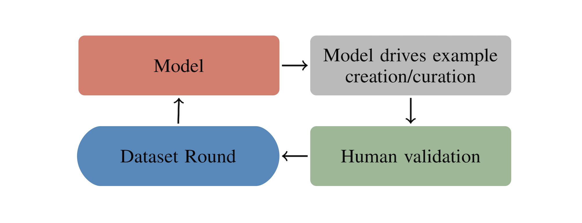
Authors: Christopher Potts*, Zhengxuan Wu*, Atticus Geiger, Douwe Kiela
Contact: cgpotts@stanford.edu
Links: Paper | Code | Video
Keywords: sentiment analysis, crowdsourcing, adversarial datasets
List of Accepted Short Papers
Attention Flows are Shapley Values
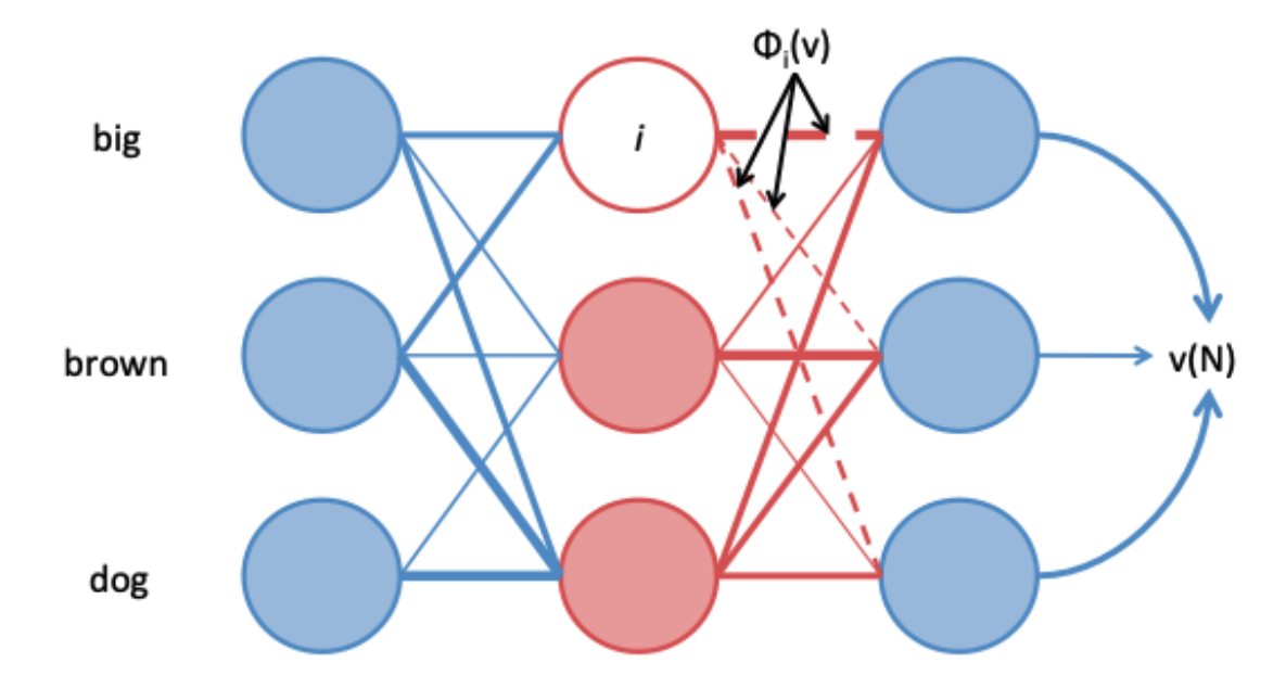
Authors: Kawin Ethyarajh, Dan Jurafsky
Contact: kawin@stanford.edu
Links: Paper
Keywords: explainability; interpretability
Question Generation for Adaptive Education
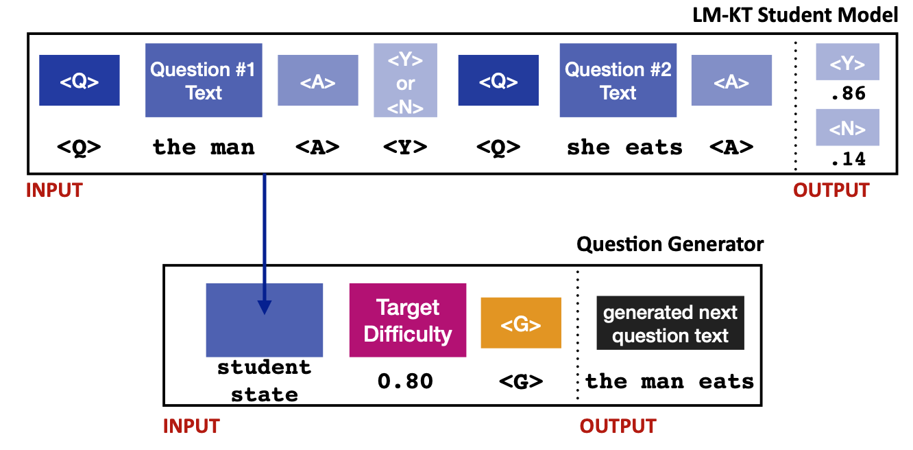
Authors: Megha Srivastava, Noah D. Goodman
Contact: meghas@stanford.edu
Links: Paper
Keywords: education, nlp, language generation
We look forward to seeing you at ACL-IJCNLP 2021!