Monthly Archives: September 2021

Posted by Elie Bursztein and Owen Vallis, Google

Today we are releasing the first version of TensorFlow Similarity, a python package designed to make it easy and fast to train similarity models using TensorFlow.

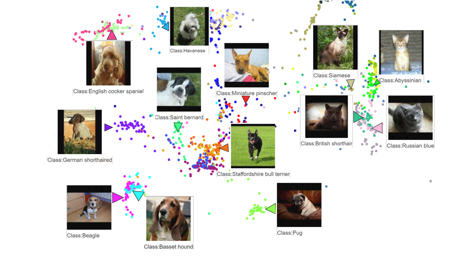
Examples of nearest neighbor searches performed on the embeddings generated by a similarity model trained on the Oxford IIIT Pet Dataset

The ability to search for related items has many real world applications, from finding similar looking clothes, to identifying the song that is currently playing, to helping rescue missing pets. More generally, being able to quickly retrieve related items is a vital part of many core information systems such as multimedia searches, recommender systems, and clustering pipelines.

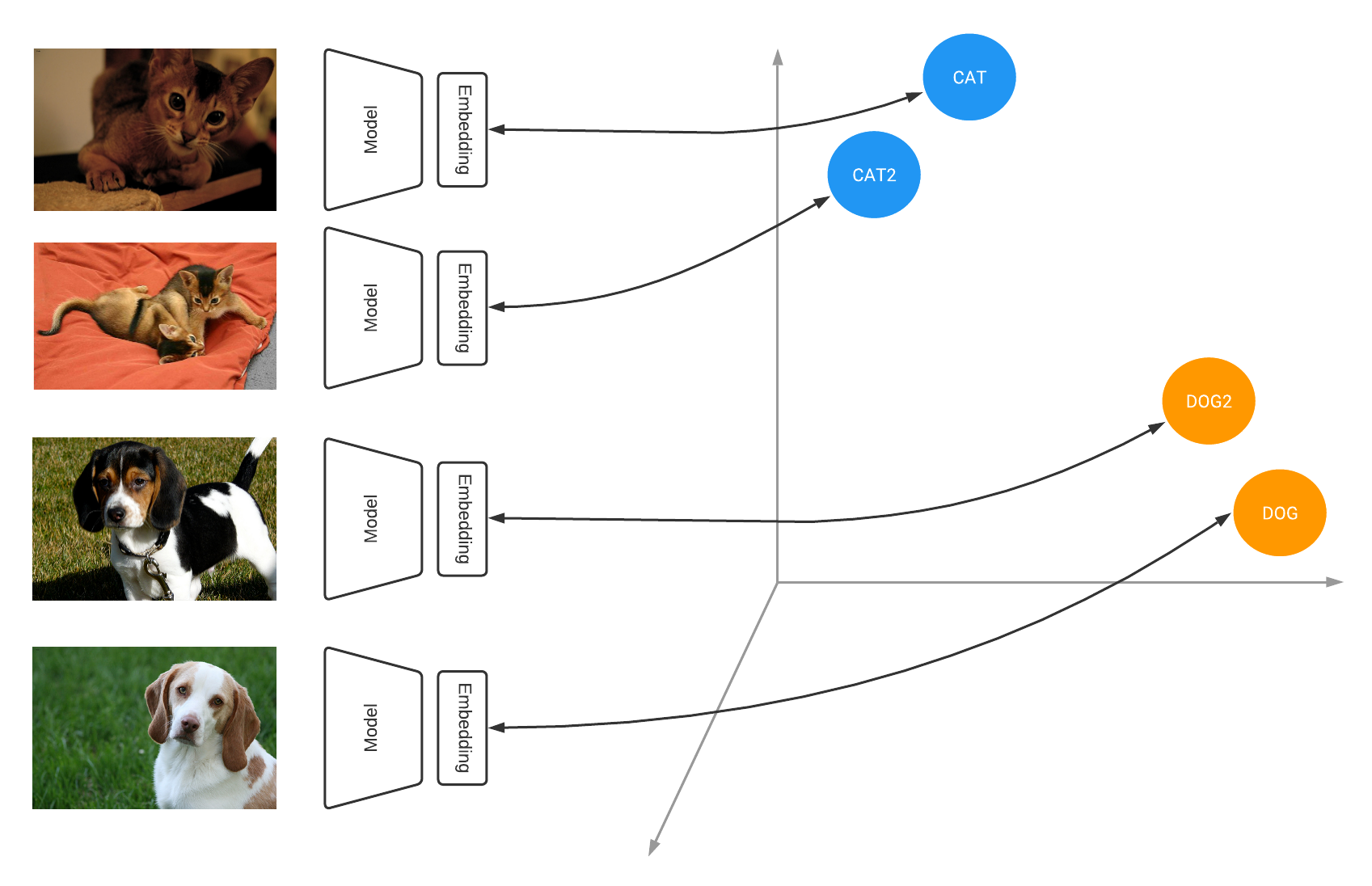Similarity models learn to output embeddings that project items in a metric space where similar items are close together and far from dissimilar ones

Under the hood, many of these systems are powered by deep learning models that are trained using contrastive learning. Contrastive learning teaches the model to learn an embedding space in which similar examples are close while dissimilar ones are far apart, e.g., images belonging to the same class are pulled together, while distinct classes are pushed apart from each other. In our example, all the images from the same animal breed are pulled together while different breeds are pushed apart from each other.

Oxford-IIIT Pet dataset visualization using the Tensorflow Similarity projector

When applied to an entire dataset, contrastive losses allow a model to learn how to project items into the embedding space such that the distances between embeddings are representative of how similar the input examples are. At the end of training you end up with a well clustered space where the distance between similar items is small and the distance between dissimilar items is large. For example, as visible above, training a similarity model on the Oxford-IIIT Pet dataset leads to meaningful clusters where similar looking breeds are close-by and cats and dogs are clearly separated.

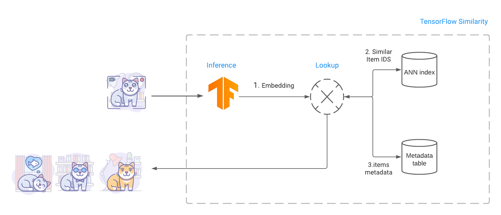Finding related items involve computing the query image embedding, performing an ANN search to find similar items and fetching similar items metadata including the images bytes.

Once the model is trained, we build an index that contains the embeddings of the various items we want to make searchable. Then at query time, TensorFlow Similarity leverages Fast Approximate Nearest Neighbor search (ANN) to retrieve the closest matching items from the index in sub-linear time. This fast look up leverages the fact that TensorFlow Similarity learns a metric embedding space where the distance between embedded points is a function of a valid distance metric. These distance metrics satisfy the triangle inequality, making the space amenable to Approximate Nearest Neighbor search and leading to high retrieval accuracy.

Other approaches, such as using model feature extraction, require the use of an exact nearest neighbor search to find related items and may not be as accurate as a trained similarity model. This prevents those methods scaling as performing an exact search requires a quadratic time in the size of the search index. In contrast, TensorFlow Similarity’s built-in Approximate Nearest Neighbor indexing system, which relies on the NMSLIB, makes it possible to search over millions of indexed items, retrieving the top-K similar matches within a fraction of second.

Beside accuracy and retrieval speed, the other major advantage of similarity models is that they allow you to add an unlimited new number of classes to the index without having to retrain. Instead you only need to compute the embeddings for representative items of the new classes and add them to the index. This ability to dynamically add new classes is particularly useful when tackling problems where the number of distinct items is unknown ahead of time, constantly changing, or is extremely large. An example of this would be enabling users to discover newly released music that is similar to songs they have liked in the past.

TensorFlow Similarity provides all the necessary components to make similarity training evaluation and querying intuitive and easy. In particular, as illustrated below, TensorFlow Similarity introduces the SimilarityModel(), a new Keras model that natively supports embedding indexing and querying. This allows you to perform end-to-end training and evaluation quickly and efficiently..

A minimal example that trains, indexes and searches on MNIST data can be written in less than 20 lines of code:

from tensorflow.keras import layers

# Embedding output layer with L2 norm
from tensorflow_similarity.layers import MetricEmbedding 
# Specialized metric loss
from tensorflow_similarity.losses import MultiSimilarityLoss 
# Sub classed keras Model with support for indexing
from tensorflow_similarity.models import SimilarityModel
# Data sampler that pulls datasets directly from tf dataset catalog
from tensorflow_similarity.samplers import TFDatasetMultiShotMemorySampler
# Nearest neighbor visualizer
from tensorflow_similarity.visualization import viz_neigbors_imgs


# Data sampler that generates balanced batches from MNIST dataset
sampler = TFDatasetMultiShotMemorySampler(dataset_name='mnist', classes_per_batch=10)

# Build a Similarity model using standard Keras layers
inputs = layers.Input(shape=(28, 28, 1))
x = layers.Rescaling(1/255)(inputs)
x = layers.Conv2D(64, 3, activation='relu')(x)
x = layers.Flatten()(x)
x = layers.Dense(64, activation='relu')(x)
outputs = MetricEmbedding(64)(x)

# Build a specialized Similarity model
model = SimilarityModel(inputs, outputs)

# Train Similarity model using contrastive loss
model.compile('adam', loss=MultiSimilarityLoss())
model.fit(sampler, epochs=5)

# Index 100 embedded MNIST examples to make them searchable
sx, sy = sampler.get_slice(0,100)
model.index(x=sx, y=sy, data=sx)

# Find the top 5 most similar indexed MNIST examples for a given example
qx, qy = sampler.get_slice(3713, 1)
nns = model.single_lookup(qx[0])

# Visualize the query example and its top 5 neighbors
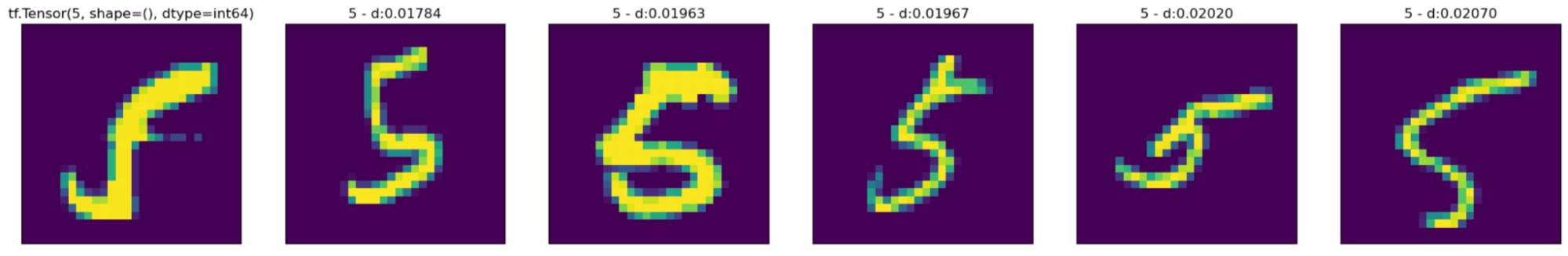
viz_neigbors_imgs(qx[0], qy[0], nns)

Even though the code snippet above uses a sub-optimal model, it still yields good matching results where the nearest neighbors clearly looks like the queried digit as visible in the screenshot below:

This initial release focuses on providing all the necessary components to help you build contrastive learning based similarity models, such as losses, indexing, batch samplers, metrics, and tutorials. TF Similarity also makes it easy to work with the Keras APIs and use the existing Keras Architectures. Moving forward, we plan to build on this solid foundation to support semi-supervised and self-supervised methods such as BYOL, SWAV, and SimCLR.

You can start experimenting with TF Similarity right away by heading to the Hello World tutorial. For more information you can check out the project Github.

Read More

Posted by Marat Dukhan and Frank Barchard, software engineers

Quantization is among the most popular methods to speedup neural network inference on CPUs. A year ago TensorFlow Lite increased performance for floating-point models with the integration of XNNPACK backend. Today, we are extending the XNNPACK backend to quantized models with, on average across computer vision models, 30% speedup on ARM64 mobile phones, 5X speedup on x86-64 laptop and desktop systems, and 20X speedup for in-browser inference with WebAssembly SIMD compared to the default TensorFlow Lite quantized kernels.

Quantized inference in XNNPACK is optimized for symmetric quantization schemas used by the TensorFlow Model Optimization Toolkit. XNNPACK supports both the traditional per-tensor quantization schema and the newer accuracy-optimized schema with per-channel quantization of weights and per-tensor quantization of activations. Additionally, XNNPACK supports the asymmetric quantization schema, albeit with reduced efficiency.

Performance improvements

We evaluated XNNPACK-acclerated quantized inference on a number of edge devices and neural network architectures. Below, we present benchmarks on four public and two internal quantized models covering common computer vision tasks:

1. EfficientNet-Lite0 image classification [download]
2. EfficientDet-Lite0 object detection [download]
3. DeepLab v3 segmentation with MobileNet v2 feature extractor [download]
4. CartoonGAN image style transfer [download]
5. Quantized version of the Face Mesh landmarks
6. Quantized version of the Video Segmentation

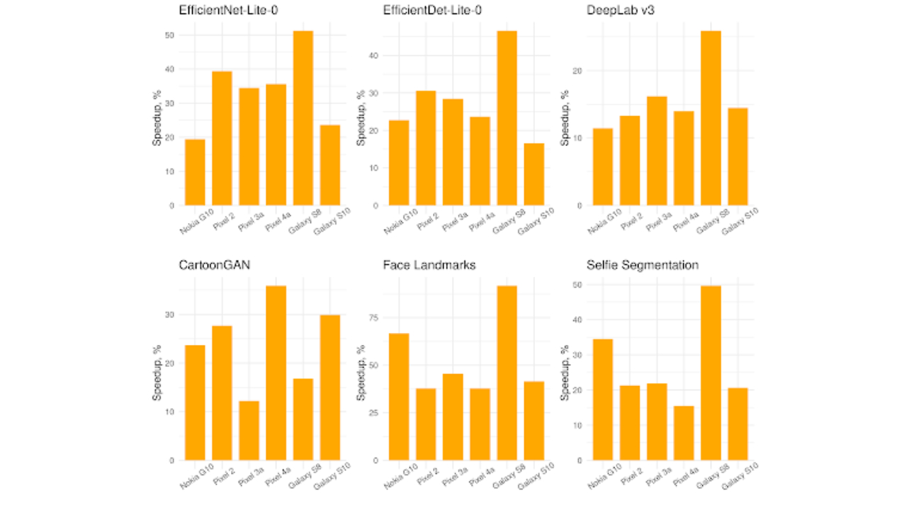
Speedup from XNNPACK on single-threaded inference of quantized computer vision models on Android/ARM64 mobile phones.

Across the six Android ARM64 mobile devices XNNPACK delivers, on average, 30% speedup over the default TensorFlow Lite quantized kernels.

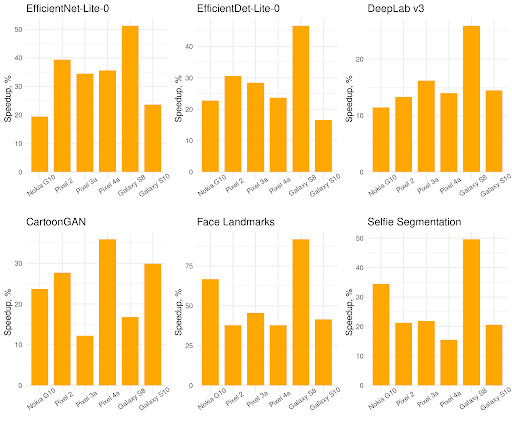
Speedup from XNNPACK on single-threaded inference of quantized computer vision models on x86-64 laptop and desktop systems.

XNNPACK offers even greater improvements on laptop and desktop systems with x86 processors. On the 5 x86 processors in our benchmarks XNNPACK accelerated inference on average by 5 times. Notably, low-end and older processors which don’t support AVX instructions see over 20X speedup from switching quantized inference to XNNPACK: while the previous TensorFlow Lite inference backend had optimized implementations only for AVX, AVX2, and AVX512 instruction sets, XNNPACK provides optimized implementations for all x86-64 processors.

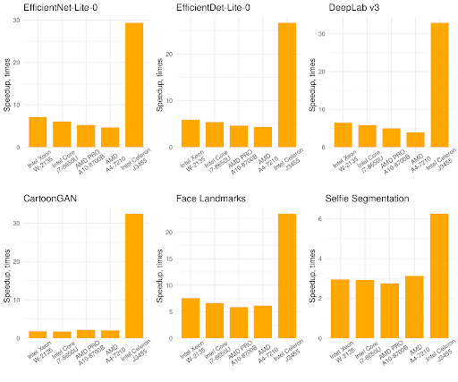
Speedup from XNNPACK on single-threaded WebAssembly SIMD inference of quantized computer vision models on mobile phones, laptops, and desktops when running through V8.

Besides the traditional mobile and laptop/desktop platforms, XNNPACK brings accelerated quantized inference to the Web platform through the TensorFlow Lite Web API. The above plot demonstrates a geomean speedup of 20X over the default TensorFlow Lite implementation when running WebAssembly SIMD benchmarks through the V8 JavaScript engine on 3 x86-64 and 2 ARM64 systems.

Two years of optimizations

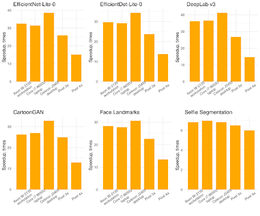
XNNPACK started its life as a fork of QNNPACK library, but as the first version of XNNPACK focused on floating-point inference and QNNPACK focused on quantized inference, it was not possible to compare the two. Now with XNNPACK introducing support for quantized inference, we can directly evaluate and attribute the two further years of performance optimizations.

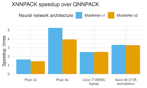
To compare the two quantized inference backends, we ported randomized MobileNet v1 and MobileNet v2 models from XNNPACK API to QNNPACK API, and benchmarked their single-threaded performance on two ARM64 Android phones and two x86-64 systems. The results are presented in the plot above, and the progress made by XNNPACK in two years is striking. XNNPACK is 50% faster on the older Pixel 3a phone and 4-5X faster on the newer Pixel 4a phone, 2.5X faster on the x86-64 laptop, and over 3X faster on the x86-64 workstation. These improvements are the result of a multiple optimizations XNNPACK gained in the two years since it forked from QNNPACK:

• XNNPACK retained the optimizations in QNNPACK, like the Indirect Convolution algorithm and microarchitecture-specific microkernel selection, and further augmented them with Indirect Deconvolution algorithm, and more flexible capabilities, like built-in numpy-like broadcasting in the quantized addition and quantized multiplication operators.
• Convolution, Deconvolution, and Fully Connected operators accumulate products of 8-bit activations and weights into a 32-bit number, and in the end this number needs to be converted back, or requantized, to an 8-bit number. There are multiple ways how requantization can be implemented, but QNNPACK adapted schema from the GEMMLOWP library, which pioneered quantized computations for neural network inference. However, it has since been discovered that GEMMLOWP requantization schema is suboptimal in terms of both accuracy and performance, and XNNPACK replaced it with more performant and accurate alternatives
• Whereas QNNPACK targeted asymmetric quantization schema, where both activations and weights are represented as unsigned integers with zero point and scale quantization parameters, XNNPACK’s optimizations focus on symmetric quantization, where both activations and weights are signed integers, and weights have additional restrictions: the zero point of the weights is always zero and the quantized weights elements are limited to the [-127, 127] range (-128 is excluded even though it can be represented as a signed 8-bit integer). Symmetric quantization offers two computational advantages exploited in XNNPACK. First, when the filter weights are static, the results of accumulating the product of input zero point by the filter weights can be completely fused into the bias term in the Convolution, Deconvolution, and Fully Connected operators. Thus, zero point parameters are completely absent from the inference computations. Secondly, the product of a signed 8-bit input element by the weight element restricted to [-127, 127] fits into 15 bits. This enables the microkernels for Convolution, Deconvolution, and Fully Connected operators to do half of the accumulations on 16-bit variables rather than always extending the products to 32 bits.
• QNNPACK microkernels were optimized NEON SIMD instructions on ARM and SSE2 SIMD instructions on x86, but XNNPACK supports a much wider set of instruction set-specific optimizations. Most quantized microkernels in XNNPACK are optimized for SSE2, SSE4.1, AVX, XOP, AVX2, and AVX512 instructions on x86/x86-64, for NEON, NEON V8, and NEON dot product instructions on ARM/ARM64, and for WebAssembly SIMD instructions. Additionally, XNNPACK provides scalar implementations for WebAssembly 1.0 and pre-NEON ARM processors.
• QNNPACK introduced the idea of specialized assembly microkernels for high-end ARM and low-end ARM cores, but XNNPACK takes this idea much further. XNNPACK not only includes specialized expert-tuned software pipelined assembly microkernels for Cortex-A53, Cortex-A55, and high-end cores with and without NEON dot product instructions, but even supports switching between them on the fly. When a thread doing inference migrates from a big to a little core, XNNPACK automatically adapts from using a microkernel optimized for the big core to the one optimized for the little core.
• QNNPACK mainly focused on multi-threaded inference and organized computations as a large number of small tasks, each computing a tiny tile of the output tensor. XNNPACK reworked parallelisation and made the tasks flexible: they can be fine-grained or coarse-grained depending on the number of threads participating in the parallelization. Through dynamic adjustment of task granularity, XNNPACK archives low overhead in single-threaded execution and high parallelization efficiency for multi-threaded inference.

Taken together, these optimizations make XNNPACK the new state-of-art for quantized inference, and turn TensorFlow Lite into the most versatile quantized inference solution, covering systems from Raspberry Pi Zero to Chromebooks to workstations with server-class processors.

How can you use it?

Quantized XNNPACK inference is enabled by default in the CMake builds of TensorFlow Lite for all platforms, in the Bazel builds of TensorFlow Lite for the Web platform, and will be available in TensorFlow Lite Web API in the 2.7 release. In Bazel builds for other platforms, quantized XNNPACK inference is enabled via a build-time opt-in mechanism. When building TensorFlow Lite with Bazel, add --define tflite_with_xnnpack=true --define xnn_enable_qs8=true, and the TensorFlow Lite interpreter will use the XNNPACK backend by default for supported operators with symmetric quantization. Limited support for operators with asymmetric quantization is available via the --define xnn_enable_qu8=true Bazel option.

Which operations are accelerated?

The XNNPACK backend currently supports a subset of quantized TensorFlow Lite operators (see documentation for details and limitations). XNNPACK supports models produced by the Model Optimization Toolkit through post-training integer quantization and quantization-aware training, but not post-training dynamic range quantization.

Future work

This is the third version of the XNNPACK integration into TensorFlow Lite following the initial release of the floating-point implementation and the subsequent release that brought sparse inference support. In the following versions we plan to add the following improvements:

• Half-precision inference on the recent ARM processors
• Sparse quantized inference.
• Even faster dense inference.

We encourage you to leave your thoughts and comments on our GitHub and StackOverflow pages, and you can ask questions on discuss.tensorflow.org

Read More

Posted by Luiz GUStavo Martins, Developer Advocate

At Google I/O, we shared a set of tutorials to help you use machine learning on audio. In this blog post you’ll find resources to help you develop and customize an audio classification model for your app, and a couple of real world examples for inspiration.

Machine learning for audio

Sound and audio are sometimes used interchangeably, but they have a key difference. Sound is in essence what you can hear while audio is the sound’s electronic representation. That’s why we usually use the term audio when talking about machine learning.

Machine Learning for audio can be used to:

• Understand speech
• Understand musical instruments
• Classify events (which bird is that?)
• Detect pitch
• Generate music

In this post we will focus on audio classification of events, a common scenario in practice with many real world applications like NOAA creating a humpback whale acoustic detector, and the Zoological Society of London using audio recognition to protect wildlife.

A number of classification models are available for you to try right now on TensorFlow Hub (YAMNet, Whale detection).

Audio recognition can also run completely on-device. For example, Android has a sound notifications feature that provides push notification for important sounds around you. It can also detect which music is playing, or even help with an ML-powered audio recorder app that can transcribe conversations on-device.

Having the models is only the beginning. Now you might ask:

• How do I use them on my app?
• How do I customize them for my audio use case?

Deploying machine learning models on-device

Imagine you have an audio classification model ready, such as a pretrained one from TF-Hub, how would you use this in a mobile app? To help you integrate audio classification into your app we created the TensorFlow Lite Task Library. The Audio Classifier component was released and you only need a couple of lines of code to add audio classification to your application:

// Initialization
val classifier = AudioClassifier.createFromFile(this, modelPath)

// Start recording
val record = classifier.createAudioRecord()
record.startRecording()

// Load latest audio samples
val tensor = classifier.createInputTensorAudio()
tensor.load(record);

// Run inference
val output = classifier.classify(tensor)

The library takes care of loading the model to memory, to create the audio recorder with the proper model specifications (sample rate, bit rate) and the classification method to get the model’s inference results. Here you can find a full sample to get some inspiration.

Customizing the models

What if you need to recognize audio events that are not in the set provided by the pretrained models? Or if you need to specialize them to fewer classes? In these situations, you need to fine tune the model using a technique called Transfer Learning.

This is a very popular process and you don’t need to be an expert on machine learning to be able to do it. You can use Model Maker to help you with this.

spec = audio_classifier.YamNetSpec()
data = audio_classifier.DataLoader.from_folder(spec, DATA_DIR)
 
train_data, validation_data = data.split(0.8)
model = audio_classifier.create(train_data, spec, validation_data)
 
model.export(models_path)

You can find complete code here. The output model can be directly loaded by the Task Library. And Model Maker can customize models not only for audio but also for image, text and recommendation system

Summary

Machine learning for audio is an exciting field and with many possibilities, enabling many new features. Doing ML on-device is getting easier and faster with tools like TensorFlow Lite Task Library and customization can be done without expertise in the field with Model Maker.

You can learn more about it on our new On-Device Machine Learning website (the audio path is here). You’ll find tutorials, codelabs and lots of resources on how to do not only audio related tasks but also for image (classification, object detection) and text (classification, entity extraction, question and answer)

You can share with us what you build by adding #TensorFlow on your social network post with your project, or submit it for the TensorFlow community spotlight program. And if you have any questions, you can ask them on discuss.tensorflow.org.

Read More