Monthly Archives: November 2021

Today, we’re excited to announce the launch of personalized recommenders in Amazon Personalize that are optimized for retail and media and entertainment, making it even easier to personalize your websites, apps, and marketing campaigns. With this launch, we have drawn on Amazon’s rich experience creating unique personalized user experiences using machine learning (ML) to build recommenders for common personalization use cases. Use cases optimized recommendation solutions deliver personalized experiences for your users that consider the metrics that matter most to your business, the preferences of your individual users, and where your users are being served a personalized experience within the user journey. You can quickly integrate recommenders into any application via easy-to-use APIs.

This post walks you through the process of creating a recommender and getting recommendations for your users.

New personalized recommenders

To realize the true potential of personalization, businesses need to tailor their content to the user journey. For instance, an ecommerce website can recommend products to an existing customer based on their past browsing history (for example, a “Recommended for you” carousel) to drive greater engagement by providing item recommendations that are relevant to that user’s individual interests. On a product detail page, you can upsell products through a “Customers who viewed X also viewed” widget that uses the context of the product your customer is already engaging with. Finally, on the checkout page, a retailer may want to cross-sell products with “Frequently bought together” recommendations to increase average order value.

Similarly, a video-on-demand business can place a widget on their home page that shows the most popular recommendations to highlight the most viewed content across the world in the past week or month. You may want to build a “Because you watched this” widget after videos are watched to provide similar content with a greater chance of driving an increase in the time spent on your platform.

Each touchpoint requires intelligent personalization that understands the user, their current context, and their real-time interests or in-session preferences when delivering recommendations. Businesses today understand the need for and benefits of personalization, but building recommendation systems from the ground up requires significant investments of time and resources, in addition to extensive ML expertise.

With the launch of recommenders, you simply select the use cases you need from a library of recommenders within Amazon Personalize. “Most Viewed,” “Best Sellers”, “Frequently Bought Together,” “Customers who Viewed X also Viewed,” and “Recommended for you” are available for retail, and “Most Popular,” “Because you Watched X,” “More Like X,” and “Top Picks” are available for media and entertainment, with more to come. You select the recommenders for your use cases and Amazon Personalize does the heavy lifting of using ML to generate recommendations that you access through an easy-to-use API.

Recommenders learn from your users’ historical activity as well as their real-time interactions with items in your catalog to adjust to changing user preferences and deliver immediate value to your end users and business. Recommenders fully manage the lifecycle of maintaining and hosting personalized recommendation solutions. This accelerates the time needed to bring a solution to market and ensures that the recommendation solutions you deliver to production stay relevant for your users.

Amazon Personalize enables developers to build personalized user experiences with the same ML technology used by Amazon with no ML expertise required. We make it easy for developers to build applications capable of delivering a wide array of personalization experiences. You can start getting recommendations with Amazon Personalize quickly using a few simple API calls or some clicks on the AWS Management Console. You only pay for what you use, with no minimum fees or upfront commitments. All data is encrypted to be private and secure, and is only used to create your recommendations and segments.

Create a recommender

This section walks through the process of creating a recommender. The first step is to create a domain dataset group, which you can create by loading historic data in Amazon Simple Storage Service (Amazon S3) or from data gathered from real-time events.

Each dataset group can contain up to three datasets: Users, Items, and Interactions, with the Interactions dataset being mandatory to create a recommender. Datasets must adhere to the domain-specific schema in order to be used to create the domain-related recommenders.

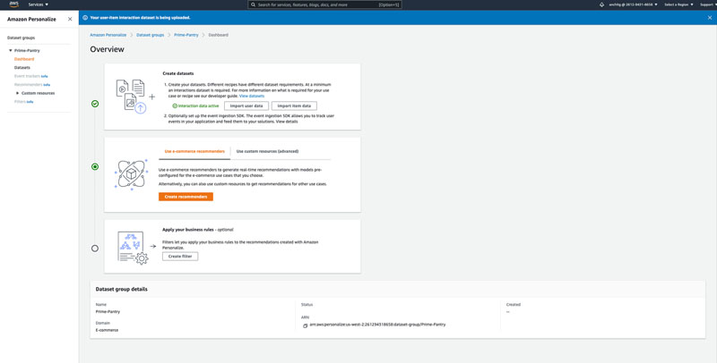
In this post, we use the Amazon Prime Pantry dataset, which consists of purchase-related data for grocery items, to set up a retail recommender. We have uploaded the interactions dataset under the dataset group Prime-Pantry. You can monitor the status of the data upload through the dashboard for the Prime-Pantry dataset group on the Amazon Personalize console. After the data is imported successfully, choose Create recommenders.

As of this writing, Amazon Personalize offers five recipes for retail customers and four for media and entertainment customers.

The retail recipes are as follows:

• Customers who viewed X also viewed – Recommendations for items that customers also viewed when they viewed a given item
• Frequently bought together – Recommendations for items that customers buy together based on a specific item
• Popular Items by Purchases – Popular items based on the items purchased by your users
• Popular Items by Views – Popular items based on items viewed by your users
• Recommended for you – Personalized recommendations for a given user ensuring that any items previously purchased are filtered out

The recipes for media and entertainment are as follows:

• Most Popular – Most popular videos
• Because you watched X – Videos similar to a given video watched by a user
• More like X – Videos similar to a given video
• Top picks for you – Personalized content recommendations for a specified user

The following screenshot shows how you can select recommenders based on your business needs and define the names of the recommenders. You use each recommender’s ARN to get recommendations when using the REST APIs. In this example, we create two recommenders. The first recommender is for the use case “Items frequently bought together” and is called PP-ItemsFrequentlyBoughtTogether. We also create a recommender for the use case “Popular Items by Purchases” called PP-PopularItemsByPurchases.

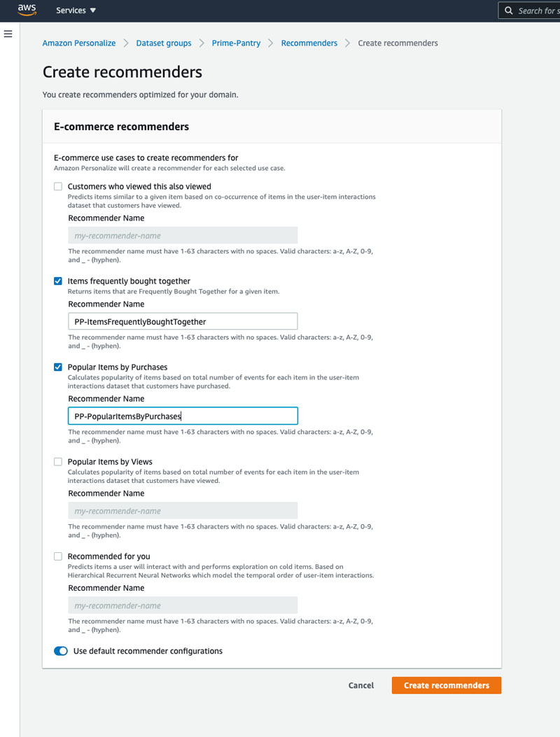
You can toggle Use default recommender configurations and Amazon Personalize automatically chooses the best configuration for the models underlying the recommenders. Then choose Create recommenders to start the model building process.

The time taken to create a recommender depends on the data and use cases selected. During this time, Amazon Personalize selects the optimal algorithm for each of the selected use cases, processes the underlying data, and trains a custom private model for your users. You can access all your recommenders and their current status on the Recommenders page.

When the recommender’s status changes to Active, you can choose it to review relevant details about the recommender and test it. Testing helps check the recommendations before you integrate the recommender into your website or application.

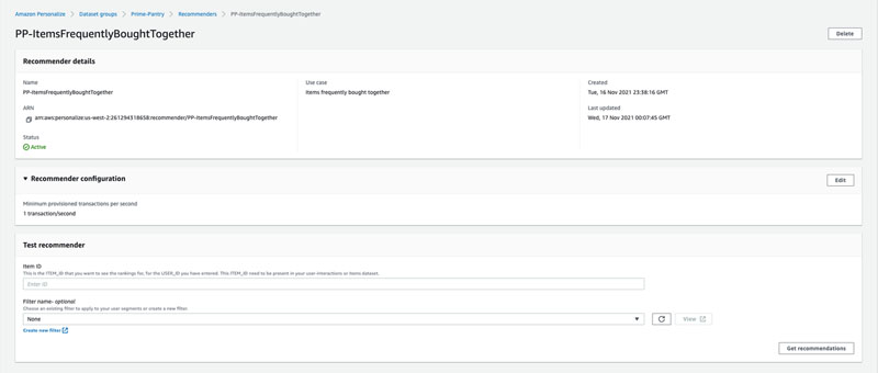
The following image shows the test output for a particular item ID for the recommender PP ItemsFrequentlyBoughtTogether.

At this step, you can also apply any filters on the recommendations; for example, to remove items purchased in the past.

Amazon Personalize also provides a recommender ARN in the details section, which you can use to produce recommendations through the Amazon Personalize REST APIs. The following code is an example of calling your API from Python for PP-FrequentlyBoughtTogetherRecommender:

get_recommendations_response = personalize_runtime.get_recommendations( 
campaignArn = arn:aws:personalize:us-west-2:261294318658:recommender/PP-ItemsFrequentlyBoughtTogether 
itemId = str(item_id) 
)

This API call produces the same results as if testing the recommender via the console.

Your recommender is now ready to feed into your website or app and personalize the journey of each of your customers.

Conclusion

Amazon Personalize packages our rich experience creating unique personalized user experiences with ML at Amazon and offers our expertise as a fully managed service to developers looking to personalize their websites and apps. With the launch of use case optimized recommenders, we’re going one step further to tailor our learnings to the unique marketing needs of each industry and each individual business. Recommenders allow you to easily and swiftly access recommendations that are optimized for your specific use case. By understanding the unique context of your customers and their touchpoints, Amazon Personalize allows you to harness the raw power of ML to derive more value for your business and your users.

To learn more about Amazon Personalize, visit the product page.

About the Authors

Anchit Gupta is a Senior Product Manager for Amazon Personalize. She focuses on delivering products that make it easier to build machine learning solutions. In her spare time, she enjoys cooking, playing board/card games, and reading.

Hao Ding is an Applied Scientist at AWS AI Labs and is working on developing next generation recommender system for Amazon Personalize. His research interests include Recommender System, Deep Learning, and Graph Mining.

Pranav Agarwal is a Sr. Software Development Engineer with Amazon Personalize and works on architecting software systems and building AI-powered recommender systems at scale. Outside of work, he enjoys reading, running and has started picking up ice-skating.

Nghia Hoang is a Senior Machine Learning Scientist at AWS AI Labs working on developing personalized learning methods with applications to recommender systems. His research interests include Probabilistic Inference, Deep Generative Learning, Personalized Federated Learning and Meta Learning.

Read More

Machine learning operations (MLOps) are key to effectively transition from an experimentation phase to production. The practice provides you the ability to create a repeatable mechanism to build, train, deploy, and manage machine learning models. To quickly adopt MLOps, you often require capabilities that use your existing toolsets and expertise. Projects in Amazon SageMaker give organizations the ability to easily set up and standardize developer environments for data scientists and CI/CD (continuous integration, continuous delivery) systems for MLOps engineers. With SageMaker projects, MLOps engineers or organization administrators can define templates that bootstrap the ML workflow with source version control, automated ML pipelines, and a set of code to quickly start iterating over ML use cases. With projects, dependency management, code repository management, build reproducibility, and artifact sharing and management become easy for organizations to set up. SageMaker projects are provisioned using AWS Service Catalog products. Your organization can use project templates to provision projects for each of your users.

In this post, you use a custom SageMaker project template to incorporate CI/CD practices with GitLab and GitLab pipelines. You automate building a model using Amazon SageMaker Pipelines for data preparation, model training, and model evaluation. SageMaker projects builds on Pipelines by implementing the model deployment steps and using SageMaker Model Registry, along with your existing CI/CD tooling, to automatically provision a CI/CD pipeline. In our use case, after the trained model is approved in the model registry, the model deployment pipeline is triggered via a GitLab pipeline.

Prerequisites

For this walkthrough, you should have the following prerequisites:

• A GitLab account
• An AWS account
• An Amazon SageMaker Studio domain (with SageMaker projects enabled)

This post provides a detailed explanation of the SageMaker projects, GitLab, and GitLab pipelines integration. We review the code and discuss the components of the solution. To deploy the solution, reference the GitHub repo, which provides step-by-step instructions for implementing a MLOps workflow using a SageMaker project template with GitLab and GitLab pipelines.

Solution overview

The following diagram shows the architecture we build using a custom SageMaker project template.

Let’s review the components of this architecture to understand the end-to-end setup:

• GitLab – Acts as our code repository and enables CI/CD using GitLab pipelines. The custom SageMaker project template creates two repositories (model build and model deploy) in your GitLab account.
  • The first repository (model build) provides code to create a multi-step model building pipeline. This includes steps for data processing, model training, model evaluation, and conditional model registration based on accuracy. It trains a linear regression model using the XGBoost algorithm on the well-known UCI Machine Learning Abalone dataset.
  • The second repository (model deploy) contains the code and configuration files for model deployment, as well as the test scripts required to pass the quality benchmark. These are code stubs that must be defined for your use case.
  • Each repository also has a GitLab CI pipeline. The model build pipeline automatically triggers and runs the pipeline from end to end whenever a new commit is made to the model build repository. The model deploy pipeline is triggered whenever a new model version is added to the model registry, and the model version status is marked as Approved.
• SageMaker Pipelines – Contains the directed acyclic graph (DAG) that includes data preparation, model training, and model evaluation.
• Amazon S3 – An Amazon Simple Storage Service (Amazon S3) bucket stores the output model artifacts that are generated from the pipeline.
• AWS Lambda – Two AWS Lambda functions are created, which we review in more detail later in this post:
  • One function seeds the code into your two GitLab repositories.
  • One function triggers the model deployment pipeline after the new model is registered in the model registry.
• SageMaker Model Registry – Tracks the model versions and respective artifacts, including the lineage and metadata. A model package group is created that contains the group of related model versions. The model registry also manages the approval status of the model version for downstream deployment.
• Amazon EventBridge – Amazon EventBridge monitors all changes to the model registry. It also contains a rule that triggers the Lambda function for the model deploy pipeline, when the model package version state changes from PendingManualApproval to Approved in the model registry.
• AWS CloudFormation – AWS CloudFormation deploys the model and creates the SageMaker endpoints when the model deploy pipeline is triggered by the approval of the trained model.
• SageMaker hosting – Creates two HTTPS real-time endpoints to perform inference. The hosting option is configurable, for example, for batch transform or asynchronous inference. The staging endpoint is created when the model deploy pipeline is triggered by the approval of the trained model. This endpoint is used to evaluate the deployed model by confirming it’s generating predictions that meet our target accuracy requirements. When the model is ready to be deployed in production, a production endpoint is provisioned by manually starting the job in the GitLab model deploy pipeline.

Use the new MLOps project template with GitLab and GitLab pipelines

In this section, we review the parameters required for the MLOps project template (see the following screenshot). This template allows you to utilize GitLab pipelines as your orchestrator.

The template has the following parameters:

• GitLab Server URL – The URL of the GitLab server in https:// format. The GitLab accounts under your organization may contain a different customized server URL (domain). The server URL is required to authorize access to the python-gitlab API. You use the personal access token you created to allow permission to the Lambda functions to push the seed code into your GitLab repositories. We discuss the Lambda function code in more detail in the next section.
• Base URL for your GitLab Repositories – The URL for your GitLab account to create the model build and deploy repositories in the format of https://<gitlab server>/<username> or https://<gitlab server><group>/<project>. You must create a personal access token under your GitLab user account in order to authenticate with the GitLab API.
• Model Build Repository Name – The name of the repository mlops-gitlab-project-seedcode-model-build of the model build and training seed code.
• Model Deploy Repository Name – The name of the repository mlops-gitlab-project-seedcode-model-deploy of the model deploy seed code.
• GitLab Group ID – GitLab groups are important for managing access and permissions for projects. Enter the ID of the group that repositories are created for. In this example, we enter None, because we’re using the root group.
• GitLab Secret Name (Secrets Manager) – The secret in AWS Secrets Manager contains the value of the GitLab personal access token that is used by the Lambda function to populate the seed code in the repositories. Enter the name of the secret you created in Secrets Manager.

Lambda functions code overview

As discussed earlier, we create two Lambda functions. The first function seeds the code into your GitLab repositories. The second function triggers your model deployment. Let’s review these functions in more detail.

Seedcodecheckin Lambda function

This function helps create the GitLab projects and repositories and pushes the code files into these repositories. These files are needed to set up the ML CI/CD pipelines.

The Secrets Manager secret is created to allow the function to retrieve the stored GitLab personal access token. This token allows the function to communicate with GitLab to create repositories and push the seed code. It also allows the environment variables to be passed in through the project.yml file. See the following code:

def get_secret():
    ''' '''
    secret_name = os.environ['SecretName']
    region_name = os.environ['Region']
    
    session = boto3.session.Session()
    client = session.client(
        service_name='secretsmanager',
        region_name=region_name
    )

The Secrets Manager secret was created when you ran the init.sh file earlier as part of the code repo prerequisites.

The deployment package for the function contains several libraries, including python-gitlab and cfn-response. Because our function’s source code is packaged as a .zip file and interacts with AWS CloudFormation, we use cfn-response. We use the python-gitlab API and the Amazon SDK for Python (Boto3) to download the seed code files and upload them to Amazon S3 to be pushed to our GitLab repositories. See the following code:

    # Configure SDKs for GitLab and S3
    gl = gitlab.Gitlab(gitlab_server_uri, private_token=gitlab_private_token)
    s3 = boto3.client('s3')
 
    model_build_filename = f'/tmp/{str(uuid.uuid4())}-model-build-seed-code.zip'
    model_deploy_filename = f'/tmp/{str(uuid.uuid4())}-model-deploy-seed-code.zip'
    model_build_directory = f'/tmp/{str(uuid.uuid4())}-model-build'
    model_deploy_directory = f'/tmp/{str(uuid.uuid4())}-model-deploy'

    # Get Model Build Seed Code from S3 for Gitlab Repo
    with open(model_build_filename, 'wb') as f:
        s3.download_fileobj(sm_seed_code_bucket, model_build_sm_seed_code_object_name, f)

    # Get Model Deploy Seed Code from S3 for Gitlab Repo
    with open(model_deploy_filename, 'wb') as f:
        s3.download_fileobj(sm_seed_code_bucket, model_deploy_sm_seed_code_object_name, f)

Two projects (repositories) are created in GitLab, and the seed code files are pushed into the repositories (model build and model deploy) using the python-gitlab API:

# Create the GitLab Project
    try:
        if group_id is None:
            build_project = gl.projects.create({'name': gitlab_project_name_build})
        else:
            build_project = gl.projects.create({'name': gitlab_project_name_build, 'namespace_id': int(group_id)})
    ....
    try:
        if group_id is None:
            deploy_project = gl.projects.create({'name': gitlab_project_name_deploy})
        else:
            deploy_project = gl.projects.create({'name': gitlab_project_name_deploy, 'namespace_id': int(group_id)})
    ....
    
    # Commit to the above created Repo all the files that were in the seed code Zip
    try:
        build_project.commits.create(build_data)
    except Exception as e:
        logging.error("Code could not be pushed to the model build repo.")
        logging.error(e)
        cfnresponse.send(event, context, cfnresponse.FAILED, response_data)
        return { 
            'message' : "GitLab seedcode checkin failed."
        }

    try:
        deploy_project.commits.create(deploy_data)
    except Exception as e:
        logging.error("Code could not be pushed to the model deploy repo.")
        logging.error(e)
        cfnresponse.send(event, context, cfnresponse.FAILED, response_data)
        return { 
            'message' : "GitLab seedcode checkin failed."
        }

The following screenshot shows the successful run of the Lambda function pushing the required seed code files into both projects in your GitLab account.

gitlab-trigger Lambda function

This Lambda function is triggered by EventBridge. The project.yml CloudFormation template contains an EventBridge rule that triggers the function when the model package state changes in the SageMaker model registry. See the following code:

ModelDeploySageMakerEventRule:
    Type: AWS::Events::Rule
    Properties:
      # Max length allowed: 64
      Name: !Sub sagemaker-${SageMakerProjectName}-${SageMakerProjectId}-event-rule # max: 10+33+15+5=63 chars
      Description: "Rule to trigger a deployment when SageMaker Model registry is updated with a new model package. For example, a new model package is registered with Registry"
      EventPattern:
        source:
          - "aws.sagemaker"
        detail-type:
          - "SageMaker Model Package State Change"
        detail:
          ModelPackageGroupName:
            - !Sub ${SageMakerProjectName}-${SageMakerProjectId}
      State: "ENABLED"
      Targets:
        -
          Arn: !GetAtt GitLabPipelineTriggerLambda.Arn
          Id: !Sub sagemaker-${SageMakerProjectName}-trigger

The following screenshot contains a subset of the function code that triggers the GitLab pipeline in the .gitlab-ci.yml file. It deploys the SageMaker model endpoints using the CloudFormation template endpoint-config-template.yml in your model deploy repository.

To better understand the solution, review the entire code for the functions as needed.

GitLab and GitLab pipelines overview

As described earlier, GitLab plays a key role as the source code repo and enabling CI/CD pipelines in this solution. Let’s look into our GitLab account to understand the components.

After the project is successfully created, using our custom template in SageMaker projects per the steps in the code repo, navigate to your GitLab account to see two new repositories. Each repository has a GitLab CI pipeline associated with it that runs as soon as the project is created.

The first run of each pipeline fails because GitLab doesn’t have the AWS credentials. For each repository, navigate to Settings, CI/CD, Variables. Create two new variables, AWS_ACCESS_KEY_ID and AWS_SECRET_ACCESS_KEY, with the associated information for your GitLab role.

Model build pipeline in GitLab

Let’s review the GitLab pipelines, starting with the model build pipeline. We define the pipelines in GitLab by creating the .gitlab-ci.yml file, where we define the various stages and related jobs. As shown in the following screenshot, this pipeline has only one stage (training) and the related script shows how a SageMaker pipeline file is triggered. (You can learn more about the SageMaker pipeline by exploring the pipeline.py file on GitHub.)

When this GitLab pipeline is triggered, it starts the Abalone SageMaker pipeline to build your model.

When the model build is complete, you can locate this model in the model registry in SageMaker Studio.

Use this template for your custom use case

The model build repository contains code for preprocessing, training, and evaluating the model for the UCI Abalone dataset. You need to modify the files to address your custom use case.

1. Navigate to the pipelines folder in your model build repository.

2. Upload your dataset to a S3 bucket. Replace the bucket URL in this section of your pipeline.py file.

3. Navigate to .gitlab-ci.yml and modify this section with the folder and file of your use case.

Model deployment pipeline in GitLab

When the SageMaker pipeline that trains the model is complete, a model is added to the SageMaker model registry. If that model is approved, the GitLab pipeline in the model deploy repository starts and the model deployment process begins.

To approve the model in the model registry, complete the following steps:

1. Choose the Components and registries icon.
2. Choose Model registry, and choose (right-click) the model version.
3. Choose Update model version status.
4. Change the status from Pending to Approved.

This triggers the deploy pipeline.

Now, let’s review the .gitlab-ci.yml file in the model deploy repository. As shown in the following screenshot, this model deploy pipeline has four stages: build, staging deploy, test staging, and production deploy. This pipeline uses AWS CloudFormation to deploy the model and create the SageMaker endpoints.

A manual step in the GitLab pipeline exists for model promotion from staging to production that creates an endpoint with the suffix -prod. If you choose manual, this job runs and upon completion deploys the SageMaker endpoint.

To verify that the endpoints were created, navigate to the Endpoints page on the SageMaker console. You should see two endpoints: <model_name>-staging and <model_name>-prod.

GitLab implementation patterns

In this section, we discuss two patterns for implementing GitLab: hosting with Amazon Virtual Private Cloud (Amazon VPC), or with two-factor authentication.

Hosting GitLab in an Amazon VPC

You may choose to deploy GitLab in an Amazon VPC to use a private network and provide access to AWS resources. In this scenario, the Lambda functions also must be deployed in a VPC to access the GitLab API. We accomplish this by updating the project.yml file and the AWS Identity and Access Management (IAM) role AmazonSageMakerServiceCatalogProductsUseRole.

The IAM user that you used to create the VPC requires the following user permissions for Lambda to verify network resources:

• ec2:DescribeSecurityGroups
• ec2:DescribeSubnets
• ec2:DescribeVpcs

The Lambda functions’ execution role requires the following permissions to create and manage network interfaces:

• ec2:CreateNetworkInterface
• ec2:DescribeNetworkInterfaces
• ec2:DeleteNetworkInterface

1. On the IAM console, search for AmazonSageMakerServiceCatalogProductsUseRole.
2. Choose Attach policies.
3. Search for the AWSLambdaVPCAccessExecutionRole managed policy.
4. Choose Attach policy.

Next, we update project.yml to configure the functions to deploy in a VPC by providing the VPC security groups and subnets.

1. 1. Add the subnet IDs and security group IDs to the Parameters section, for example:

      SubnetId1:
      Type: AWS::EC2::Subnet::Id
      Description: Subnet Id for Lambda function
      
      SubnetId2:
      Type: AWS::EC2::Subnet::Id
      Description: Subnet Id for Lambda function
      
      SecurityGroupId:
      Type: AWS::EC2::SecurityGroup::Id
      Description: Security Group Id for Lambda function to Execute
      

   2. Add the VpcConfig information under Properties for the GitSeedCodeCheckinLambda and GitLabPipelineTriggerLambda functions, for example:

      SubnetId1:
      GitSeedCodeCheckinLambda:
      Type: 'AWS::Lambda::Function'
      Properties:
      Description: To trigger the codebuild project for the seedcode checkin
      .....
      VpcConfig:
      SecurityGroupIds:
      - !Ref SecurityGroupId
      SubnetIds:
      - !Ref SubnetId1
      - !Ref SubnetId2
      

Two-factor authentication enabled

If you enabled two-factor authentication on your GitLab account, you need to use your personal access token to clone the repositories in SageMaker Studio. The token requires the read_repository and write_repository flags. To clone the model build and model deploy repositories, enter the following commands:

git clone https://oauth2:PERSONAL_ACCESS_TOKEN@gitlab.com/username/gitlab-project-seedcode-model-build-<project-id>
git clone https://oauth2:PERSONAL_ACCESS_TOKEN@gitlab.com/username/gitlab-project-seedcode-model-deploy-<project-id>

Read More

This is a guest post by Lucas Baker, Andrea Duque, and Viet Yen Nguyen of Hypefactors.  

At Hypefactors, we build tech for media intelligence and reputation management. The solution is a software as a service (SaaS) product that does large-scale media monitoring of social media, news sites, TV, radio, and reviews across the world. The tracked data is streamed continuously and enriched in real time. This yields insights that can reveal early business opportunities (for example, GameStop hype), track the success of product launches, and preempt disasters.

To this end, over a hundred million network requests are made daily from data pipelines for web crawling, social media firehoses, and other REST-based media data integrations. This yields millions of new articles and posts each day. This data can be segmented into three classes (as illustrated with the following examples):

• Owned – Articles or posts written by a company and published on their own website or social media feed.
• Paid – Information written by a company and published on third-party websites or social media. This is known colloquially as advertisement.
• Earned – Information written by a third party and published on that party’s website or social media.

Owned media	Earned media	Paid media

Differentiating between earned articles and owned or paid ones is of existential importance. Earned information is more independent and therefore interpreted as more trustworthy—no matter if it’s positive or negative for the company. Advertisement, on the other hand, is written by the company and portrays the best interests of the company. Therefore, to accurately track reputation, we must filter out advertisements.

This post goes deeper into our deep learning natural language processing (NLP) based advertisement predictor, how we integrated the predictor into one of our pipelines using Deep Java Library (DJL), and how that change made our architecture simpler and MLOps easier. DJL is an open source Java framework for deep learning created by AWS.

Printed newspapers and magazines: Challenges

We receive thousands of different magazines and newspapers directly from publishing houses in the form of digital files. One of the data teams within Hypefactors has developed a data pipeline, which we call the Print-ETL. The Print-ETL processes the raw data and ingests it into a database. The ingested data is made searchable in a user-friendly way by the Hypefactors web platform.

Processing and realigning data from different data providers is generally challenging. This is also the case with handling different publishing houses as data providers. The challenges are technical, organizational, and a combination thereof. That is partly because media houses are legacy both in their data delivery and data formats.

Organizational challenges include disagreement between different media houses on how media data should be delivered, and the lack of a common schema. A common strategy media houses use is to provide print data via an SFTP server. This can be consumed by periodically connecting and fetching the data. Most of the time we retrieve only the digital PDF files of the editions, but they can also arrive in other formats, such as XML or ZIP. On top of that, files often come with no relevant metadata about the publication. Such metadata is useful, for example, to identify the title of the newspaper or the magazine.

The technical challenges are various. However, when it comes to PDFs, one of the biggest challenges is that a PDF may or may not be vectorized. A vectorized PDF, as opposed to a bitmapped one, is one that contains all the raw data that appears on the page. When a PDF is vectorized, it’s easy to retrieve its text. But when it’s not, all we have are bitmapped images. To make articles searchable for users, the content of a bitmapped PDF needs to be transformed to a text format using optical character recognition (OCR) solutions.

Another big challenge is that PDFs can have any number of pages. Typically, there is no information telling us which pages constitute an article. There can be several articles sharing one PDF page, or several PDF pages containing a single article. Advertisements also appear anywhere—they can cover the whole page, several pages, or just a small section close to an article.

To mitigate these difficulties, we developed elaborate development and operations procedures. These are assisted by automated procedures, such as automated unit and end-to-end testing, as well as automated testing, staging, and production rollouts. Operations therefore play an essential role to keep the overall solution running.

Print-ETL architecture

The data pipeline processes events, in which each event contains a file retrieved from a media house. These events are processed in a distributed and concurrent manner by subscribing to a message topic. We use Monix, a Scala library for asynchronous computation, to process the events with high performance. Ideally, we process data as soon as it arrives, but we don’t have control over when data is released. Therefore, we have periodic peak loads of these events. At other times, there are no events at all. The whole system is deployed in the cloud to make use of its elasticity. Cloud instances are auto scaled proportionally to the number of events received, so naturally the more data we receive, the more resources we use to process that data.

The Print-ETL uses deep learning and other AI techniques to solve most print media challenges and extract the relevant information out of the raw print data. There are several AI and machine learning (ML) models in place. These include computer vision models (for page segmentation) and NLP models (for ad prediction, headline detection, and next sentence prediction).

Today’s practices are that deploying deep learning models incurs complexity by itself. Correspondingly, new practices come into the spotlight for managing the ML lifecycle in production reliably and efficiently—the emerging field of MLOps. In our use case, we use Deep Java Library (DJL) to integrate ML models into our data pipelines written in Scala. We found that this strategy simplifies model deployment and maintenance alike. In this post, we focus on the model we use to filter paid advertisements: the ad predictor.

The following diagram illustrates the Print-ETL architecture.

First version ad predictor: Serverless inference

We approached the advertisement classification challenge as a supervised binary text classification problem. We fine-tuned a BERT (Bidirectional Encoder Representations from Transformers) pre-trained multilingual base model with a binary classification layer on top of the transformer output. For training, we used a custom-built dataset containing advertisement data that we collected. The input of the model is a sequence of tokens, and the output is a classification score from 0–1, which is the probability of being an ad. This score is calculated by applying a sigmoid function to the linear layer prediction outputs (logits).

On our first iteration, we deployed a standalone ad predictor endpoint on an external service. This made operations harder. Predictions had a higher latency because of network calls and boot up times, causing timeouts and issues resulting from predictor unavailability due to instance interruptions. We also had to auto scale both the data pipeline and the prediction service, which was non-trivial given the unpredictable load of events. However, this strategy also had a few benefits. The service was packaged separately as an API and developed in Python, a language more familiar to data scientists than Scala. Also, the predictor wasn’t integrated into the Print-ETL system, so it wasn’t necessary to be familiar with the system to maintain the predictor.

The following diagram illustrates our BERT model for text classification.

The following is an example of our ads data.

Second version with DJL

Our solution to these challenges centered on combining the benefits of two frameworks: Open Neural Network Exchange (ONNX) and Deep Java Library.

With ONNX and DJL, we deployed a new multilingual ad predictor model directly in our pipeline. This replaced our first solution, the serverless ad predictor. The new model was fine-tuned on a new, larger set of data that contained over 450,000 sentences in Danish, English, and Portuguese. They reflect a sample of the production data being processed at the moment.

When deploying the model, DJL enabled us to adopt an API-free strategy. This strategy improved our data processing in myriad ways. For instance, it helped us achieve our latency requirements and use ML inferences in real time. Also, by replacing our standalone ad predictor, we no longer needed to mock an external service API in our tests. That allowed us to simplify our test suite. This in turn led to more test stability. Following our successful deployment, DJL allowed us to integrate other ML models that improved data processing even further.

Let’s go into the details of ONNX and DJL.

ONNX

ONNX is an open-source ecosystem of AI and ML tools designed to provide extensive interoperability between different deep learning frameworks. It manages models from different languages and environments. Their tools and common file format enable us to train a model using one framework, dynamically quantize it using tools from another, and deploy that model using yet another framework. That increased interoperability, along with help from DJL, allowed us to easily integrate our model with the JVM—and consequently our Scala pipeline as well.

More specifically, we used a tool called ONNX Runtime. We converted our original PyTorch model to the standard ONNX file format, and then applied dynamic quantization techniques using ONNX Runtime. This shrunk our original model size by about a factor of four with little to no loss in model performance. It also gave our model a speed boost on CPU-based inferences. In particular, from prior rollouts we had simple, yet cost-effective performance with 8 bits quantization when running a CPU with AVX-512 instructions. We were confident that this strategy would give us the results we were looking for.

Deep Java Library

DJL presented the other half of our solution. DJL is an open-source library that defines a Java-based deep learning framework. DJL abstracts away complexities involved with deep learning deployments, making training and inference a breeze. It’s engine agnostic, and is therefore compatible with a wide variety of deep learning engines. Those engines include PyTorch, TensorFlow, and MXNet, among others. Most importantly for us, DJL supports the ONNX Runtime engine.

Our DJL-based deployment brought several advantages over our original ad predictor deployment. First and foremost, from an engineering perspective, it was simpler. The direct native integration of ad prediction with our Scala data pipeline streamlined our architecture considerably. It allowed us to avoid the computational overhead of serializing and deserializing data, as well as the latency of making network calls to an external service.

Additionally, this meant that there was no longer any need for complicated autoscaling of an external service—the pipeline’s existing autoscaling infrastructure was sufficient to meet all our data processing requirements. Moreover, DJL’s predictor architecture worked well with Monix’s concurrent data processing, allowing us to make multiple inferences simultaneously across different threads.

Those simplifications led us to eliminate our standalone ad predictor service entirely. This eliminated all operational costs associated with running and maintaining that service.

Another consequence of those simplifications was the further streamlining of our test suite. For example, we no longer needed to mock our ad predictor. We could instead directly ensure the correctness and performance of our model on every commit using our continuous integration (CI). Upon every new commit pushed to the Print-ETL, our CI would run our suite of tests, which included tests for the DJL-based ad predictor. This maintains our confidence that our deep learning model works properly whenever we change our code base.

The following screenshot is a snippet of our ad detection CI in action.

Our testing strategy is now twofold: first, we use tests to determine the validity of our ad predictor model’s output; namely, the model should detect the same ads with the same, or higher, level of accuracy as previous iterations of the model. Second, the model’s robustness is stressed by passing particularly long, short, strange, or fragmented text samples. End-to-end performance tests that take advantage of the ad predictor’s services add a second layer of accountability. This makes sure that current and future deployments of our ad predictor function as intended. If the ad predictor isn’t performing as expected, our tests immediately reflect that incapability. The following code is an example of some sample test cases:

  /** Some sample test cases */
  it should "detect ads in danish, english, and portuguese" in {
    val daAdSentence = "Lidt bedre end andre gode oste"
    val daAdLikelihood = AdDetector.predict(daAdSentence)
    daAdLikelihood.success.value should be > 0.9d

    val enAdSentence = "Save 10% when you buy in the next ten minutes!"
    val enAdLikelihood = AdDetector.predict(enAdSentence)
    enAdLikelihood.success.value should be > 0.9d

    val ptAdSentence = "Defenda a sua saúde, tomando YOGHURT"
    val ptAdLikelihood = AdDetector.predict(ptAdSentence)
    ptAdLikelihood.success.value should be > 0.9d
  }

This, in turn, simplified our operations strategy as well. It’s now easier to spot, track, and reproduce inference errors if and when they occur. Such an error immediately tells us which input the model failed to predict on, the exact error message given by ONNX Runtime, along with relevant information for reproducing the error. Also, because our ad predictor is now integrated with our data pipeline, we only need to consult one log stream when analyzing error messages. After the associated bug is reproduced and fixed, we can add a new test case to ensure the same bug doesn’t occur again.

Conclusion and next steps

We have been happy with our DJL-based deployment. Our success with DJL has empowered us to utilize the same strategy to deploy other deep learning models for other purposes, such as headline detection and next sentence prediction. In each of those cases, we experienced similar results as with our ad predictor—deployment was easy, simple, and economical.

In the future, one avenue we would be excited to explore with DJL is GPU-based inference. Our current DJL deployments are exclusively CPU based—partially due to its cost-effectiveness, and partially due to its simplicity when compared to a GPU-based alternative. Given our experiences with DJL, however, we believe that DJL could drastically streamline any GPU-based deployment that we pursue. To learn more and get started on DJL, visit the website. You can also visit the GitHub repo, demo repository, examples, Slack channel, and Twitter for more documentation and examples of DJL!

The content and opinions in this post are those of the third-party author and AWS is not responsible for the content or accuracy of this post.

About the Authors

Lukas Baker works in the intersection of data engineering and applied machine learning. At Hypefactors, he occasionally builds a data pipeline and designs and trains a model in between.

Andrea Duque is an all-round engineer and scientist with a history of connecting the dots with MLOps. At Hypefactors, she designs and rollouts ML-heavy data pipelines end-to-end.

Viet Yen Nguyen is the CTO of Hypefactors and leads the teams on data science, web app development and data engineering. Prior to Hypefactors, he developed technology for designing mission-critical systems, including the European Space Agency.

Read More

This post was co-written with Kevin O’Brien, Senior Data Scientist in Careem’s Integrity Team.

Dubai-based Careem became the Middle East’s first unicorn when it was acquired by Uber for $3.1 billion in 2019. A pioneer of the region’s ride-hailing economy, Careem is now expanding its services to include mass transportation, delivery, and payments as an everyday super app.

But its size and popularity—it has around 50 million customer accounts—have also made it a prime target for fraudsters constantly looking for new loopholes to exploit and different ways to hijack genuine accounts.

In this post, we share how Careem detects identity fraud using graph-based deep learning and Amazon Neptune.

The challenge

Due to Careem’s massive popularity, fraudsters are constantly looking for new loopholes to exploit, create identity-faked accounts (first-party fraud), and different ways to hijack genuine accounts—also known as account takeover (third-party fraud). In Careem’s data science and analytics backed Integrity team, they needed more advanced ways to detect and stop losses from fraud that may be damaging to both their revenue and brand reputation. This solution would ideally cover both first- and third-party fraud.

Traditionally, tackling these different kinds of fraudulent activities was a never-ending game of cat and mouse. Careem’s Integrity team would often create rules or machine learning (ML) models for each specific type of fraud, but this was sometimes problematic on two levels:

• It only allowed them to identify and block an account after the fraud had been committed and detected, which means the money had already been lost
• Fraudsters were quickly able to find a new loophole to exploit once an existing fraud pattern had been detected

As a result, instead of continuously creating overly specific tools to detect very specific fraud patterns, they wanted to build an intelligent system that was almost a blanket detection mechanism over all users, wherever they were performing actions on the platform.

The new approach

Careem needed to be proactive rather than reactive. A smarter and faster way to detect fraudulent activities and stop them before the act was committed was required.

After much experimentation, Careem decided to focus on the identity of users, and came up with a powerful way to outsmart any efforts of identity fraud. They opted to use a graph structure as a way of mapping different aspects and data points of each user’s identity together, and more importantly, characteristics shared across the identities of different users. This would allow them to detect potentially fraudulent patterns in real time across user and account activity.

Architecture overview

Before we dive deep into how Careem used Neptune an identity graph for fraud detection, let’s look at the current architecture underpinning the solution. Careem chose AWS and its automated real-time analysis and monitoring capabilities due to the existing integrated cloud setup they already had.

Data ingestion

Data ingestion comprises two stages: a one-time extract, transform, and load (ETL) for all historical data, and a live streaming service of real-time data.

• Historical data – Careem uses Apache Hive running on Amazon Simple Storage Service (Amazon S3) to extract data and push it to Amazon EMR with PySpark. Amazon EMR pushes this historical data to Neptune.
• Real-time data – Careem uses their existing event processor to feed the data from all actions performed by users through Amazon Simple Queue Service (Amazon SQS). These events are consumed by a Python interface running on AWS Elastic Beanstalk, which takes these events and writes them to Neptune in real time.

Data querying

The data ingested from these sources is then queried, again using the Python interface running on Elastic Beanstalk. A simple set of logical rules is used to process the data returned for a query on a particular user, and a decision is made on whether the action performed was likely to be done by a fraudster. Based on the value of the user’s historical transaction, the fraudulent account is either blocked automatically, if it’s a low-value customer, or sent for manual review, if they’re a high-value customer.

Data consumption

The Integrity team at Careem developed a data consumption API that is used by the other teams at Careem to query users in the graph to retrieve data about their identities.

Implementing the graph data model on Neptune

The basic building blocks of any directed graph are vertices (or nodes) and edges. A vertex is an object that represents an entity in your data. For example, a customer can be a node, and the features and information about this customer are called node properties. An edge represents a connection between different nodes. For example, we may have an edge with a label called has_device that connects a customer node to a device node. A large collection of different nodes and edges are called a graph, as illustrated in the following diagram.

One type of graph architecture is called an identity graph. Identity graphs provide a single unified view of different identities by linking multiple node identifiers such as device IDs, IP addresses, emails, or credit cards to a known person or anonymous profile using privacy-compliant methods. Typically, identity graphs are part of a larger identity resolution architecture. Identity resolution is the process of matching a human identity across a set of devices used by the same person or a household of persons for the purposes of building a representative identity, or known attributes. We can then use this identity graph to find patterns in our data that could indicate fraud activities. We can evaluate identities in the context of other identities or transactions and determine if constellations of data in the graph represent fraudulent activity.

The task we are solving in this case is called node classification. Node classification is a supervised ML approach whereby we predict the categorical feature of a node property. In this case, we decided to build a graph model to predict the is_fraud property of customer nodes using Amazon Neptune ML. Neptune ML is a feature in Neptune that makes it easy to build and train ML models on large graphs using graph neural networks (GNNs). It uses Amazon SageMaker and the Deep Graph Library (DGL) to scale the training and tuning of the graph model.

Data labeling strategy and maturity

In addition to building the graph from different data sources, we needed a robust data labeling and data maturity strategy for the supervised learning task. Data maturity is the process of making sure that the fraud labels have had sufficient time to mature. In other words, enough time has passed to ensure legitimate and fraud records have been correctly and accurately identified. The maturity period can vary depending on the business. For example, for chargeback fraud, it can take somewhere between 30 days and 2 months to accurately identify fraudulent events.

Careem’s customer nodes in the graph were labeled as fraudulent if they had historically been blocked for fraud either manually or by another one of Careem’s automated fraud detection systems that are rule based. These labels are added to the graph either in the historical ETL, for users who are already blocked, or in live streaming, which blocks users in real time. They ensured the maturity of these labels by only using fraud labels for blocked users who hadn’t contacted customer care requesting for their block to be reviewed within a period of time after being blocked.

One issue that arose was that there were many fraudulent accounts that had gone undetected. The volume of these mislabeled customer nodes was substantial enough to affect training performance of the model. To combat this, a strict set of heuristics, based on domain knowledge of the platform, was applied to the customers in the graph, which allowed a large number of these labels to be corrected using a script in the training dataset with high confidence. This allowed more accurate learning of the model due to a reduction in noisy labels.

Collaboration with AWS on Neptune ML

Throughout this project, Careem’s Integrity team worked closely with the AWS ML Specialist and Neptune ML teams to develop this project with maximum efficiency and effectiveness. This included first-hand, on-call support and troubleshooting, as well as working together to build, scale, and optimize our graph.

In addition, Careem has a large volume of properties on the edges in their graph, which were previously not being used in the model’s training and predictions. Careem provided input on the development of a modified version of the RGCN architecture in Neptune ML, which uses edge properties from the graph to learn representations, not just node properties alone, which is what the traditional RGCN model does. Throughout this process, the Neptune ML team also worked on critical features that enabled Careem to train and optimize the graph at scale. These features include multi-GPU training, custom performance metrics, training instance size estimation, scalable and parallel processing, and hyperparameters custom tuning. All of these features are available now in the latest Neptune ML release, which became generally available as of July 2021.

Looking to the future

Careem is currently working with the AWS team to build and train a deep learning model to more accurately detect fraud on their user identity graph. Testing results for the initial phase are looking promising so far, with a precision of around 85% and a recall of over 50%. In other words, the model is able to correctly identify over 50% of all users that have ever historically been blocked for fraud on the platform, with an accuracy of 85%. All of this without knowing anything about the user’s transaction history, bookings, food and grocery orders, and other details—just data about their identity.

Work is now being done to deploy this trained model to production, allowing it to detect fraud in cases such as when a fraudster sets up a new account or compromises the account of an existing genuine user. This will all be done as users perform actions in real time.

In the future, Careem also plans to add Captains (what Careem’s drivers are known as) to the graph to similarly detect fraudulent Captains, or even fraudulent activity produced by collusion between users and Captains. To learn more about Amazon Neptune ML, visit the website.

About the Authors

Kevin O’Brien is a Senior Data Scientist at Careem. He is a member of the Integrity team, whose goal is to detect and prevent fraud on the platform, through data science and analytics. Kevin leads the Identity Risk squad of the Integrity team.

Waleed (Will) Badr is a Principal AI/ML Specialist Solutions Architect who works as part of the global Amazon Machine Learning team. Will has an extensive experience in fraud detection and prevention systems and is passionate about using technology in innovative ways to positively impact the community.

Kamran Habib is a Senior Solutions Architect who works with our Digital Native Business (DNB) customers in the Middle East and North Africa (MENA) region. Kamran’s technical expertise focuses on Containers, Networking and Security and he is passionate about solving customer’s business problems with innovative technical solutions. In his spare time, he enjoys travel, listening to podcasts and cricket.

Read More