Teams in Aachen are conducting research and development in all aspects of conversational AI and natural-language processing to allow Alexa to understand user requests more accurately, in more languages, and for a more diverse set of skills.Read More
Los Angeles
Scientists in the Los Angeles area, including offices in Culver City and Pasadena, have a particular focus on research related to Amazon Prime Video and Amazon Studios, as well as developing new products.Read More
Investing in Eastern Europe’s AI future
It was an honor and a privilege to attend a special event in the Bulgarian capital, Sofia, today to launch INSAIT, the Institute for Computer Science, Artificial Intelligence and Technology. INSAIT is a new AI and computer science research institute that will provide truly world-class facilities.
It’s fantastic to see the country where I was born leading the charge in bridging Eastern Europe to the world-stage in computer science research.
The institute is modeled on the computer science departments of renowned institutions such as MIT, UC Berkeley and the Max-Planck Institute, and is backed by the Bulgarian government with an endowment fund of nearly $100 million. Its computer science and AI research will span topics such as machine learning, quantum computing, information security, robotics and many more. Within two years, INSAIT expects faculty and students to publish papers in top conferences.
Google is investing $3 million over the next three years to provide INSAIT with cloud computing resources and access to itsTensor Processing Unit Research Cloud, a specialized infrastructure for running high-performance machine learning models. Supported with additional investment from DeepMind and Amazon Web Services, INSAIT aims to attract and develop the best researchers, engineers and top PhD and MSc students.
I know there’s no shortage of talented researchers, computer scientists and engineers in Eastern Europe – indeed, Sofia is already ranked asone of Europe’s top tech cities – but historically, the lack of local facilities, funding and support has meant limited opportunities for basic research. INSAIT has been created in partnership with two of the world’s leading technology universities, ETH Zurich and EPFL Lausanne, and its supervisory and advisory boards consist of leading researchers who are committed to help the institute achieve its ambitious goals.
INSAIT opens in September, and I know the team is particularly keen to receive applications from women and other groups that are often underrepresented in the world of tech.
Google is delighted to support these efforts, and I cannot wait to see what new innovation emerges from this promising venture.
Large-Scale Matrix Factorization on TPUs
Matrix factorization is one of the oldest, yet still widely used, techniques for learning how to recommend items such as songs or movies from user ratings. In its basic form, it approximates a large, sparse (i.e., mostly empty) matrix of user-item interactions with a product of two smaller, denser matrices representing learned item and user features. These dense matrices, in turn, can be used to recommend items to a user with which they haven’t interacted before.
Despite its algorithmic simplicity, matrix factorization can still achieve competitive performance in recommender benchmarks. Alternating least squares (ALS), and especially its implicit variation, is a fundamental algorithm to learn the parameters of matrix factorization. ALS is known for its high efficiency because it scales linearly in the number of rows, columns and non-zeros. Hence, this algorithm is very well suited for large-scale challenges. But, for very large real-world matrix factorization datasets, a single machine implementation would not suffice, and so, it would require a large distributed system. Most of the distributed implementations of matrix factorization that employ ALS leverage off-the-shelf CPU devices, and rightfully so, due to the inherently sparse nature of the problem (the input matrix is mostly empty).
On the other hand, recent success of deep learning, which has exhibited growing computational capacity, has spurred a new wave of research and progress on hardware accelerators such as Tensor Processing Units (TPUs). TPUs afford domain specific hardware speedups, especially for use cases like deep learning, which involves a large number of dense matrix multiplications. In particular, they allow significant speedups for traditional data-parallel workloads, such as training models with Stochastic Gradient Descent (SGD) in SPMD (single program multiple data) fashion. The SPMD approach has gained popularity in computations like training neural networks with gradient descent algorithms, and can be used for both data-parallel and model-parallel computations, where we distribute parameters of the model across available devices. Nevertheless, while TPUs have been enormously attractive for methods based on SGD, it is not immediately clear if a high performance implementation of ALS, which requires a large number of distributed sparse matrix multiplies, can be developed for a large-scale cluster of TPU devices.
In “ALX: Large Scale Matrix Factorization on TPUs”, we explore a distributed ALS design that makes efficient use of the TPU architecture and can scale well to matrix factorization problems of the order of billions of rows and columns by scaling the number of available TPU cores. The approach we propose leverages a combination of model and data parallelism, where each TPU core both stores a portion of the embedding table and trains over a unique slice of data, grouped in mini-batches. In order to spur future research on large-scale matrix factorization methods and to illustrate the scalability properties of our own implementation, we also built and released a real world web link prediction dataset called WebGraph.
Dense Batching for Improved Efficiency
We designed ALX specifically for TPUs, exploiting unique properties of TPU architecture while overcoming a few interesting limitations. For instance, each TPU core has limited memory and restricts all tensors to have a static shape, but each example in a mini-batch can have a wildly varying number of items (i.e., inputs can be long and sparse). To resolve this, we break exceedingly long examples into multiple smaller examples of the same shape, a process called dense batching. More details about dense batching can be found in our paper.
 |
| Illustrating example of how sparse batches are densified to increase efficiency on TPUs. |
Uniform Sharding of Embedding Tables
With the batching problem solved, we next want to factorize a sparse matrix into two dense embedding matrices (e.g., user and item embeddings) such that the resulting dot product of embeddings approximate the original sparse matrix — this helps us infer predictions for all the positions from the original matrix, including those that were empty, which can be used to recommend items with which users haven’t interacted. Both the resulting embedding tables (W and H in the figure below) can potentially be too large to fit in a single TPU core, thus requiring a distributed training setup for most large-scale use cases.
Most previous attempts of distributed matrix factorization use a parameter server architecture where the model parameters are stored on highly available servers, and the training data is processed in parallel by workers that are solely responsible for the learning task. In our case, since each TPU core has identical compute and memory, it’s wasteful to only use either memory for storing model parameters or compute for training. Thus, we designed our system such that each core is used to do both.
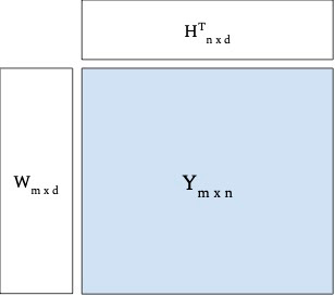 |
| Illustrative example of factorizing a sparse matrix Y into two dense embedding matrices W and H. |
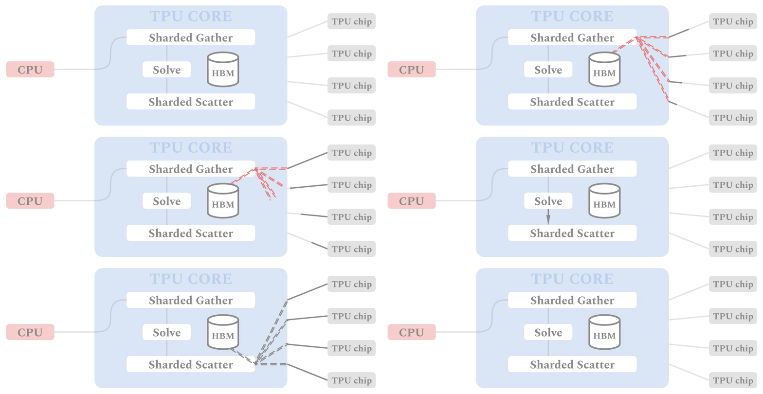
In ALX, we uniformly divide both embedding tables, thus fully exploiting both the size of distributed memory available and the dedicated low-latency interconnects between TPUs. This is highly efficient for very large embedding tables and results in good performance for distributed gather and scatter operations.
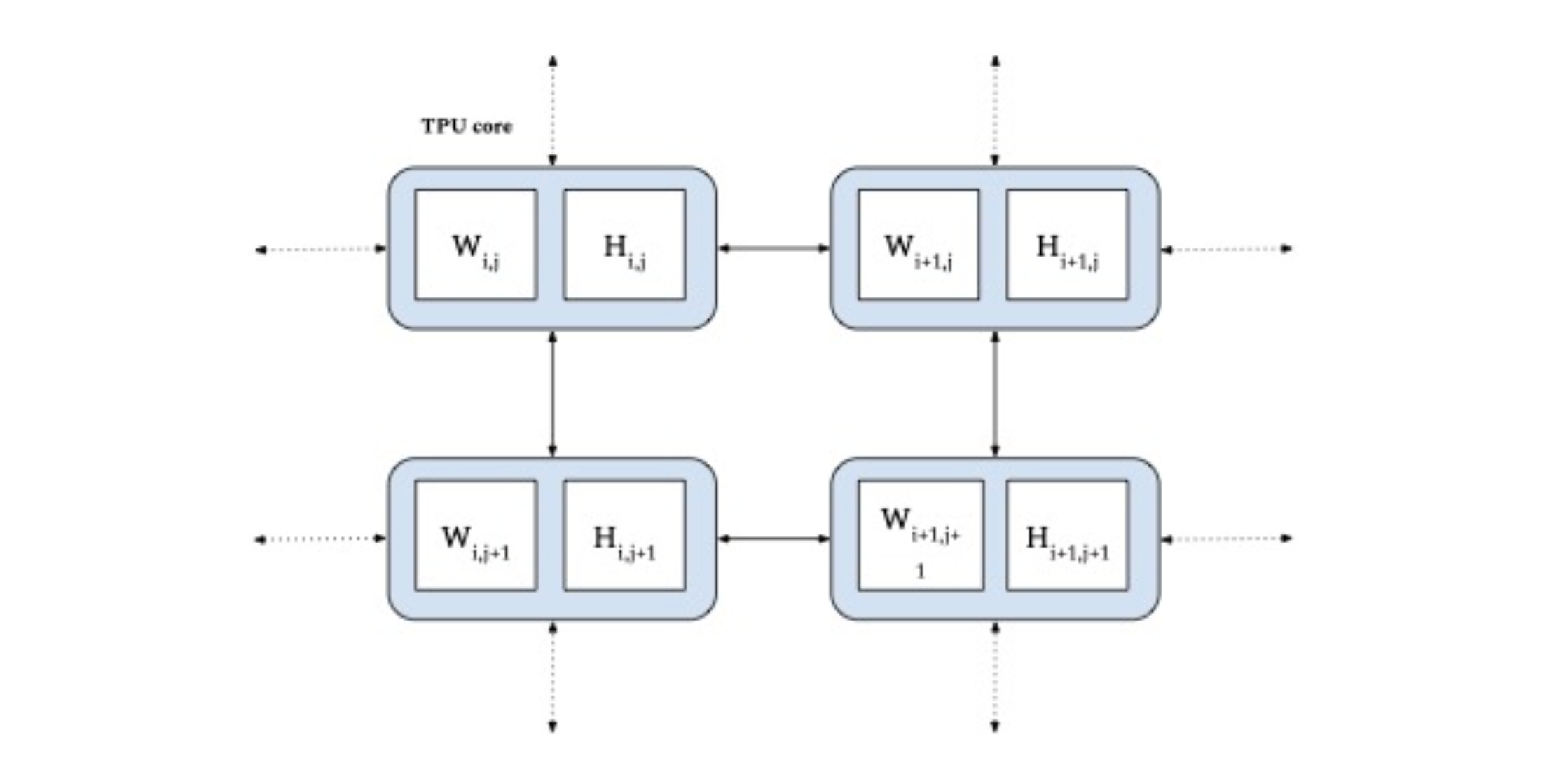 |
| Uniform sharding of both embedding tables (W and H) across TPU cores (in blue). |
WebGraph
Since potential applications may involve very large data sets, scalability is potentially an important opportunity for advancement in matrix factorization. To that end, we also release a large real-world web link prediction dataset called WebGraph. This dataset can be easily modeled as a matrix factorization problem where rows and columns are source and destination links, respectively, and the task is to predict destination links from each source link. We use WebGraph to illustrate the scaling properties of ALX.
The WebGraph dataset was generated from a single crawl performed by CommonCrawl in 2021 where we strip everything and keep only the link->outlinks data. Since the performance of a factorization method depends on the properties of the underlying graph, we created six versions of WebGraph, each varying in the sparsity pattern and locale, to study how well ALS performs on each.
- To study locale-specific graphs, we filter based on two top level domains: ‘de’ and ‘in’, each producing a graph with an order of magnitude fewer nodes.
- These graphs can still have arbitrary sparsity patterns and dangling links. Thus we further filter the nodes in each graph to have a minimum of either 10 or 50 inlinks and outlinks.
For easy access, we have made these available as a Tensorflow Dataset package. For reference, the biggest version, WebGraph-sparse, has more than 365M nodes and 30B edges. We create and publish both training and testing splits for evaluation purposes.
Results
We carefully tune the system and quality parameters of ALX. Based on our observations related to precision and choice of linear solvers. We observed that by carefully selecting the precision for storage of the embedding tables (bfloat16) and for the input to the linear solvers (float32), we were able to halve the memory required for the embeddings while still avoiding problems arising from lower precision values during the solve stage. For our linear solvers, we selected conjugate gradients, which we found to be the fastest across the board on TPUs. We use embeddings of dimension 128 and train the model for 16 epochs. In our experience, hyperparameter tuning over both norm penalty (λ) and unobserved weight (α) has been indispensable for good recall metrics as shown in the table below.
 |
| Results obtained by running ALX on all versions of WebGraph dataset. Recall values of 1.0 denote perfect recall. |
Scaling Analysis
Since the input data are processed in parallel across TPU cores, increasing the number of cores decreases training time, ideally in a linear fashion. But at the same time, a larger number of cores requires more network communication (due to the sharded embedding tables). Thanks to high-speed interconnects, this overhead can be negligible for a small number of cores, but as the number of cores increases, the overhead eventually slows down the ideal linear scaling.
In order to confirm our hypothesis, we analyze scaling properties of the four biggest WebGraph variants in terms of training time as we increase the number of available TPU cores. As shown below, even empirically, we do observe the predicted linear decrease in training time up to a sweet spot, after which the network overhead slows the decline.
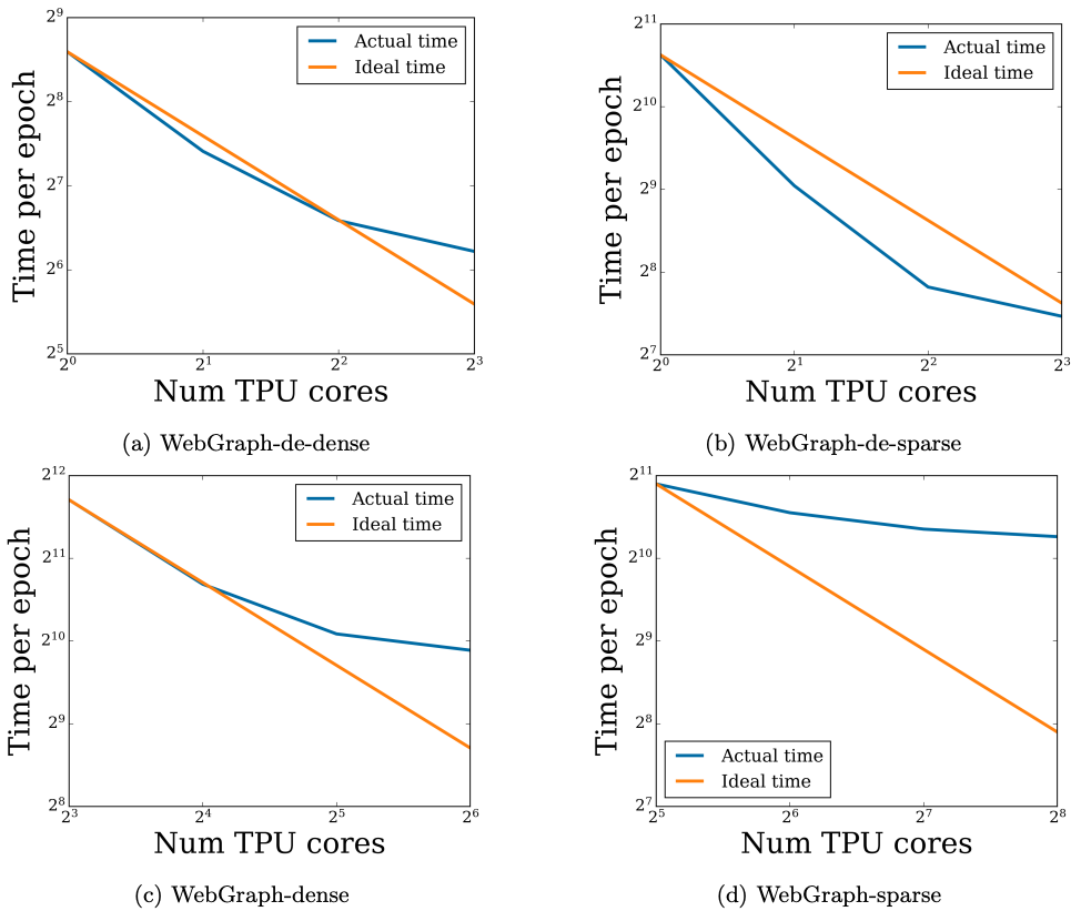 |
| Scaling analysis of running time as the number of TPU cores are increased. Each figure plots the time taken to train for one epoch in seconds. |
Conclusion
For easy access and reproducibility, the ALX code is open-sourced and can be easily run on Google Cloud. In fact, we illustrate that a sparse matrix like WebGraph-dense of size 135M x 135M (with 22B edges) can be factorized in a colab connected to 8 TPU cores in less than a day. We have designed the ALX framework with scalability in mind. With 256 TPU cores, one epoch of the largest WebGraph variant, WebGraph-sparse (365M x 365M sparse matrix) takes around 20 minutes to finish (5.5 hours for the whole training run). The final model has around 100B parameters. We hope that the ALX and WebGraph will be useful to both researchers and practitioners working in these fields. The code for ALX can be found here on github!
Acknowledgements
The core team includes Steffen Rendle, Walid Krichene and Li Zhang. We thank many Google colleagues for helping at various stages of this project. In particular, we are grateful to the JAX team for numerous discussions, especially James Bradbury and Skye Wanderman-Milne; Blake Hechtman for help with XLA and Rasmus Larsen for useful discussions about performance of linear solvers on TPUs. Finally, we’re also grateful to Nicolas Mayoraz and John Anderson for providing useful feedback.
Rock On: Scientists Use AI to Improve Sequestering Carbon Underground
A team of scientists have created a new AI-based tool to help lock up greenhouse gases like CO2 in porous rock formations faster and more precisely than ever before.
Carbon capture technology, also referred to as carbon sequestration, is a climate change mitigation method that redirects CO2 emitted from power plants back underground. While doing so, scientists must avoid excessive pressure buildup caused by injecting CO2 into the rock, which can fracture geological formations and leak carbon into aquifers above the site, or even into the atmosphere.
A new neural operator architecture named U-FNO simulates pressure levels during carbon storage in a fraction of a second while doubling accuracy on certain tasks, helping scientists find optimal injection rates and sites. It was unveiled this week in a study published in Advances in Water Resources, with co-authors from Stanford University, California Institute of Technology, Purdue University and NVIDIA.
Carbon capture and storage is one of few methods that industries such as refining, cement and steel could use to decarbonize and achieve emission reduction goals. Over a hundred carbon capture and storage facilities are under construction worldwide.
U-FNO will be used to accelerate carbon storage predictions for ExxonMobil, which funded the study.
“Reservoir simulators are intensive computer models that engineers and scientists use to study multiphase flows and other complex physical phenomena in the subsurface geology of the earth,” said James V. White, subsurface carbon storage manager at ExxonMobil. “Machine learning techniques such as those used in this work provide a robust pathway to quantifying uncertainties in large-scale subsurface flow models such as carbon capture and sequestration and ultimately facilitate better decision-making.”
How Carbon Storage Scientists Use Machine Learning
Scientists use carbon storage simulations to select the right injection sites and rates, control pressure buildup, maximize storage efficiency and ensure the injection activity doesn’t fracture the rock formation. For a successful storage project, it’s also important to understand the carbon dioxide plume — the spread of CO2 through the ground.
Traditional simulators for carbon sequestration are time-consuming and computationally expensive. Machine learning models provide similar accuracy levels while dramatically shrinking the time and costs required.
Based on the U-Net neural network and Fourier neural operator architecture, known as FNO, U-FNO provides more accurate predictions of gas saturation and pressure buildup. Compared to using a state-of-the-art convolutional neural network for the task, U-FNO is twice as accurate while requiring just a third of the training data.
“Our machine learning method for scientific modeling is fundamentally different from standard neural networks, where we typically work with images of a fixed resolution,” said paper co-author Anima Anandkumar, director of machine learning research at NVIDIA and Bren professor in the Computing + Mathematical Sciences Department at Caltech. “In scientific modeling, we have varying resolutions depending on how and where we sample. Our model can generalize well across different resolutions without the need for re-training, achieving enormous speedups.”
Trained U-FNO models are available in a web application to provide real-time predictions for carbon storage projects.
“Recent innovations in AI, with techniques such as FNOs, can accelerate computations by orders of magnitude, taking an important step in helping scale carbon capture and storage technologies,” said Ranveer Chandra, managing director of research for industry at Microsoft and collaborator on the Northern Lights initiative, a full-scale carbon capture and storage project in Norway. “Our model-parallel FNO can scale to realistic 3D problem sizes using the distributed memory of many NVIDIA Tensor Core GPUs.”
Novel Neural Operators Accelerate CO2 Storage Predictions
U-FNO enables scientists to simulate how pressure levels will build up and where CO2 will spread throughout the 30 years of injection. GPU acceleration with U-FNO makes it possible to run these 30-year simulations in a hundredth of a second on a single NVIDIA A100 Tensor Core GPU, instead of 10 minutes using traditional methods.
With GPU-accelerated machine learning, researchers can now also rapidly simulate many injection locations. Without this tool, choosing sites is like a shot in the dark.
The U-FNO model focuses on modeling plume migration and pressure during the injection process — when there’s the highest risk of overshooting the amount of CO2 injected. It was developed using NVIDIA A100 GPUs in the Sherlock computing cluster at Stanford.
“For net zero to be achievable, we will need low-emission energy sources as well as negative-emissions technologies, such as carbon capture and storage,” said Farah Hariri, a collaborator on U-FNO and technical lead on climate change mitigation projects for NVIDIA’s Earth-2, which will be the world’s first AI digital twin supercomputer. “By applying Fourier neural operators to carbon storage, we showed how AI can help accelerate the process of climate change mitigation. Earth-2 will leverage those techniques.”
Read more about U-FNO on the NVIDIA Technical Blog.
Earth-2 will use FNO-like models to tackle challenges in climate science and contribute to global climate change mitigation efforts. Learn more about Earth-2 and AI models used for climate science in NVIDIA founder and CEO Jensen Huang’s GTC keynote address:
The post Rock On: Scientists Use AI to Improve Sequestering Carbon Underground appeared first on NVIDIA Blog.
Build a custom entity recognizer for PDF documents using Amazon Comprehend
In many industries, it’s critical to extract custom entities from documents in a timely manner. This can be challenging. Insurance claims, for example, often contain dozens of important attributes (such as dates, names, locations, and reports) sprinkled across lengthy and dense documents. Manually scanning and extracting such information can be error-prone and time-consuming. Rule-based software can help, but ultimately is too rigid to adapt to the many varying document types and layouts.
To help automate and speed up this process, you can use Amazon Comprehend to detect custom entities quickly and accurately by using machine learning (ML). This approach is flexible and accurate, because the system can adapt to new documents by using what it has learned in the past. Until recently, however, this capability could only be applied to plain text documents, which meant that positional information was lost when converting the documents from their native format. To address this, it was recently announced that Amazon Comprehend can extract custom entities in PDFs, images, and Word file formats.
In this post, we walk through a concrete example from the insurance industry of how you can build a custom recognizer using PDF annotations.
Solution overview
We walk you through the following high-level steps:
- Create PDF annotations.
- Use the PDF annotations to train a custom model using the Python API.
- Obtain evaluation metrics from the trained model.
- Perform inference on an unseen document.
By the end of this post, we want to be able to send a raw PDF document to our trained model, and have it output a structured file with information about our labels of interest. In particular, we train our model to detect the following five entities that we chose because of their relevance to insurance claims: DateOfForm, DateOfLoss, NameOfInsured, LocationOfLoss, and InsuredMailingAddress. After reading the structured output, we can visualize the label information directly on the PDF document, as in the following image.
This post is accompanied by a Jupyter notebook that contains the same steps. Feel free to follow along while running the steps in that notebook. Note that you need to set up the Amazon SageMaker environment to allow Amazon Comprehend to read from Amazon Simple Storage Service (Amazon S3) as described at the top of the notebook.
Create PDF annotations
To create annotations for PDF documents, you can use Amazon SageMaker Ground Truth, a fully managed data labeling service that makes it easy to build highly accurate training datasets for ML.
For this tutorial, we have already annotated the PDFs in their native form (without converting to plain text) using Ground Truth. The Ground Truth job generates three paths we need for training our custom Amazon Comprehend model:
- Sources – The path to the input PDFs.
- Annotations – The path to the annotation JSON files containing the labeled entity information.
- Manifest – The file that points to the location of the annotations and source PDFs. This file is used to create an Amazon Comprehend custom entity recognition training job and train a custom model.
The following screenshot shows a sample annotation.
The custom Ground Truth job generates a PDF annotation that captures block-level information about the entity. Such block-level information provides the precise positional coordinates of the entity (with the child blocks representing each word within the entity block). This is distinct from a standard Ground Truth job in which the data in the PDF is flattened to textual format and only offset information—but not precise coordinate information—is captured during annotation. The rich positional information we obtain with this custom annotation paradigm allows us to train a more accurate model.
The manifest that’s generated from this type of job is called an augmented manifest, as opposed to a CSV that’s used for standard annotations. For more information, see Annotations.
Use the PDF annotations to train a custom model using the Python API
An augmented manifest file must be formatted in JSON Lines format. In JSON Lines format, each line in the file is a complete JSON object followed by a newline separator.
The following code is an entry within this augmented manifest file.
A few things to note:
- Five labeling types are associated with this job:
DateOfForm,DateOfLoss,NameOfInsured,LocationOfLoss, andInsuredMailingAddress. - The manifest file references both the source PDF location and the annotation location.
- Metadata about the annotation job (such as creation date) is captured.
-
Use-textract-onlyis set toFalse, meaning the annotation tool decides whether to use PDFPlumber (for a native PDF) or Amazon Textract (for a scanned PDF). If set totrue, Amazon Textract is used in either case (which is more costly but potentially more accurate).
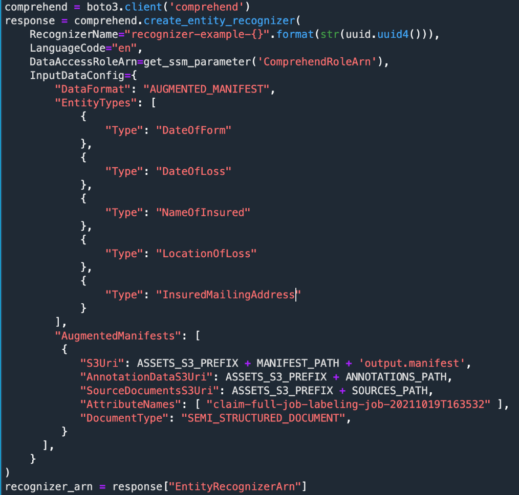
Now we can train the recognizer, as shown in the following example code.
We create a recognizer to recognize all five types of entities. We could have used a subset of these entities if we preferred. You can use up to 25 entities.
For the details of each parameter, refer to create_entity_recognizer.
Depending on the size of the training set, training time can vary. For this dataset, training takes approximately 1 hour. To monitor the status of the training job, you can use the describe_entity_recognizer API.
Obtain evaluation metrics from the trained model
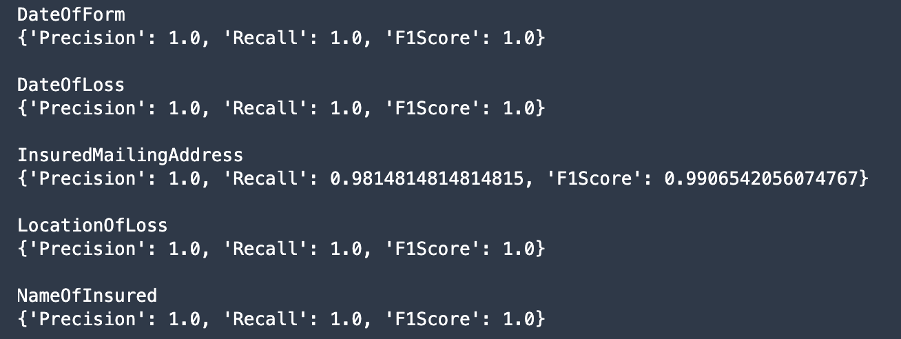
Amazon Comprehend provides model performance metrics for a trained model, which indicates how well the trained model is expected to make predictions using similar inputs. We can obtain both global precision and recall metrics as well as per-entity metrics. An accurate model has high precision and high recall. High precision means the model is usually correct when it indicates a particular label; high recall means that the model found most of the labels. F1 is a composite metric (harmonic mean) of these measures, and is therefore high when both components are high. For a detailed description of the metrics, see Custom Entity Recognizer Metrics.
When you provide the documents to the training job, Amazon Comprehend automatically separates them into a train and test set. When the model has reached TRAINED status, you can use the describe_entity_recognizer API again to obtain the evaluation metrics on the test set.
The following is an example of global metrics.
The following is an example of per-entity metrics.
The high scores indicate that the model has learned well how to detect these entities.
Perform inference on an unseen document
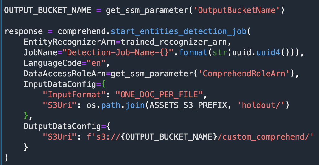
Let’s run inference with our trained model on a document that was not part of the training procedure. We can use this asynchronous API for standard or custom NER. If using it for custom NER (as in this post), we must pass the ARN of the trained model.
We can review the submitted job by printing the response.
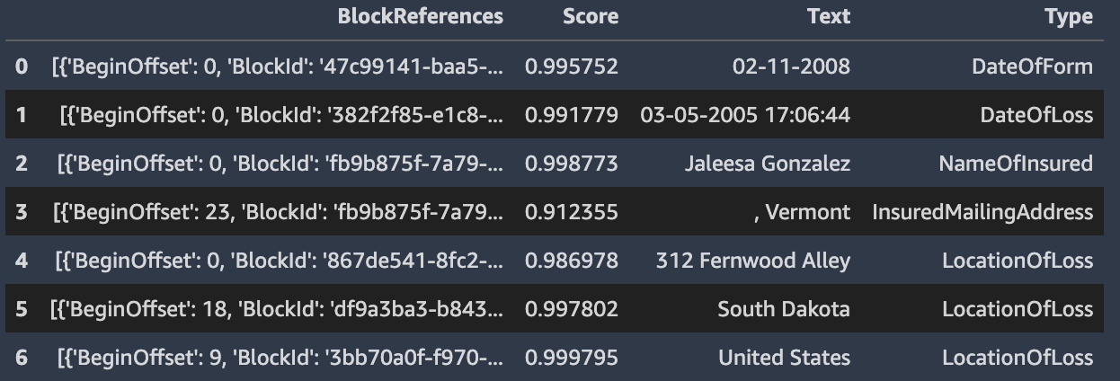
We can format the output of the detection job with Pandas into a table. The Score value indicates the confidence level the model has about the entity.
Finally, we can overlay the predictions on the unseen documents, which gives the result as shown at the top of this post.
Conclusion
In this post, you saw how to extract custom entities in their native PDF format using Amazon Comprehend. As next steps, consider diving deeper:
- Train your own recognizer using the accompanying notebook here. Remember to delete any resources when finished to avoid future charges.
- Set up your own custom annotation job to collect PDF annotations for your entities of interest. For more information, refer to Custom document annotation for extracting named entities in documents using Amazon Comprehend.
- Train a custom NER model on the Amazon Comprehend console. For more information, see Extract custom entities from documents in their native format with Amazon Comprehend.
About the Authors
 Joshua Levy is Senior Applied Scientist in the Amazon Machine Learning Solutions lab, where he helps customers design and build AI/ML solutions to solve key business problems.
 Andrew Ang is a Machine Learning Engineer in the Amazon Machine Learning Solutions Lab, where he helps customers from a diverse spectrum of industries identify and build AI/ML solutions to solve their most pressing business problems. Outside of work he enjoys watching travel & food vlogs.
 Alex Chirayath is a Software Engineer in the Amazon Machine Learning Solutions Lab focusing on building use case-based solutions that show customers how to unlock the power of AWS AI/ML services to solve real world business problems.
 Jennifer Zhu is an Applied Scientist from Amazon AI Machine Learning Solutions Lab. She works with AWS’s customers building AI/ML solutions for their high-priority business needs.
 Niharika Jayanthi is a Front End Engineer in the Amazon Machine Learning Solutions Lab – Human in the Loop team. She helps create user experience solutions for Amazon SageMaker Ground Truth customers.
 Boris Aronchik is a Manager in Amazon AI Machine Learning Solutions Lab where he leads a team of ML Scientists and Engineers to help AWS customers realize business goals leveraging AI/ML solutions.
Vocal Effort Modeling in Neural TTS for Improving the Intelligibility of Synthetic Speech in Noise
We present a neural text-to-speech (TTS) method that models natural vocal effort variation to improve the intelligibility of synthetic speech in the presence of noise. The method consists of first measuring the spectral tilt of unlabeled conventional speech data, and then conditioning a neural TTS model with normalized spectral tilt among other prosodic factors. Changing the spectral tilt parameter and keeping other prosodic factors unchanged enables effective vocal effort control at synthesis time independent of other prosodic factors. By extrapolation of the spectral tilt values beyond what…Apple Machine Learning Research
Getting started with the Amazon Kendra Box connector
Amazon Kendra is a highly accurate and easy-to-use intelligent search service powered by machine learning (ML). Amazon Kendra offers a suite of data source connectors to simplify the process of ingesting and indexing your content, wherever it resides.
For many organizations, Box Content Cloud is a core part of their content storage and lifecycle management strategy. An enterprise Box account often contains a treasure trove of assets, such as documents, presentations, knowledge articles, and more. Now, with the new Amazon Kendra data source connector for Box, these assets and any associated tasks or comments can be indexed by Amazon Kendra’s intelligent search service to reveal content and unlock answers in response to users’ queries.
In this post, we show you how to set up the new Amazon Kendra Box connector to selectively index content from your Box Enterprise repository.
Solution overview
The solution consists of the following high-level steps:
- Create a Box app for Amazon Kendra via the Box Developer Console.
- Add sample documents to your Box account.
- Create a Box data source via the Amazon Kendra console.
- Index the sample documents from the Box account.
Prerequisites
To try out the Amazon Kendra connector for Box, you need the following:
- An AWS account with privileges to create AWS Identity and Access Management (IAM) roles and policies. For more information, see Overview of access management: Permissions and policies.
- Basic knowledge of AWS and working knowledge of Box Enterprise administration.
- Admin access to a Box Enterprise workspace.
Create a Box app for Amazon Kendra
Before you configure an Amazon Kendra Box data source connector, you must first create a Box app.
- Log in to the Box Enterprise Developer Console.
- Choose Create New App.

- Choose Custom App.

- Choose Server Authentication (with JWT).
- Enter a name for your app. For example,
KendraConnector. - Choose Create App.

- In your created app in My Apps, choose the Configuration tab.
- In the App Access Level section, choose App + Enterprise Access.

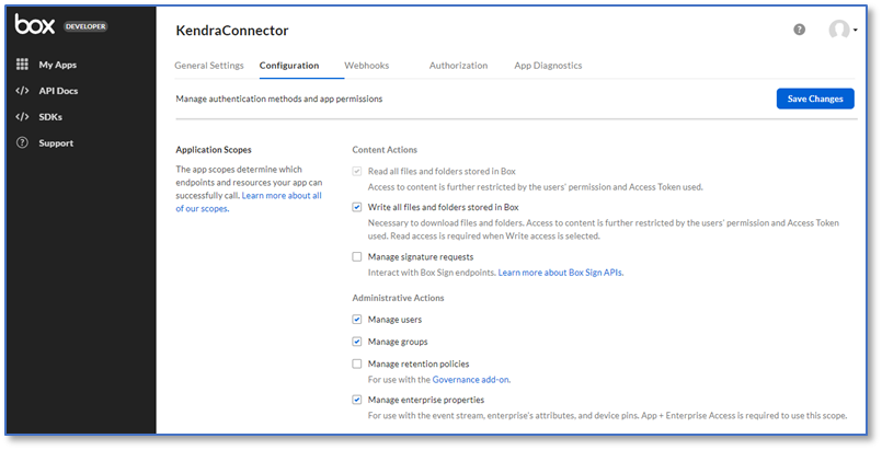
- In the Application Scopes section, check that the following permissions are enabled:
- In the Advanced Features section, select Make API calls using the as-user header.
- In the Add and Manage Public Keys section, choose Generate a Public/Private Keypair.

This requires two-step verification. A JSON text file is downloaded to your computer.
- Choose OK to accept this download.

- Choose Save Changes.
- On the Authorization tab, choose Review and Submit.
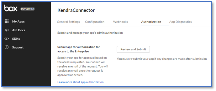
- Select Submit app within this enterprise and choose Submit.
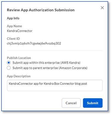
Your Box Enterprise owner needs to approve the app before you can use it.
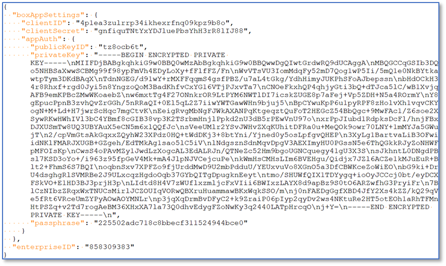
Go to the downloads directory on your computer to review the downloaded JSON file. It contains the client ID, client secret, public key ID, private key, pass phrase, and enterprise ID. You need these values to create the Box data source in a later step.
Add sample documents to your Box account
In this step, you upload sample documents to your Box account. Later, we use the Amazon Kendra Box data source to crawl and index these documents.
- Download AWS_Whitepapers.zip to your computer.
- Extract the files to a folder called
AWS_Whitepapers.

- Upload the
AWS_Whitepapersfolder to your Box account.

Create a Box data source
To add a data source to your Amazon Kendra index using the Box connector, you can use an existing Amazon Kendra index, or create a new Amazon Kendra index. Then complete the following steps to create a Box data source:
- On the Amazon Kendra console, choose Indexes in the navigation pane.
- From the list of indexes, choose the index that you want to add the data source to.
- Choose Add data sources.
- From the list of data source connectors, choose Add connector under Box.
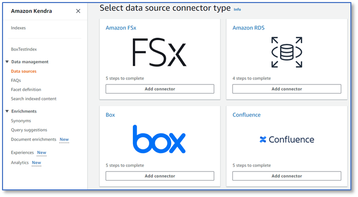
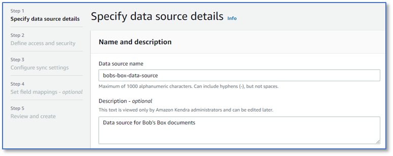
- On the Specify data source details page, enter a data source name and optional description.
- Choose Next.
- Open the JSON file you downloaded from the Box Developer Console.
It contains values for clientID, clientSecret, publicKeyID, privateKey, passphrase, and enterpriseID.
- On the Define access and security page, in the Source section, for Box enterprise ID, enter the value of the
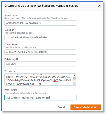
enterpriseIDfield. - In the Authentication section, under AWS Secrets Manager secret, choose Create and add a new secret.
- For Secret name, enter a name for the secret, for example,
boxsecret1. - For the remaining fields, enter the corresponding values from the downloaded JSON file.
- Choose Save and add secret.
- In the IAM role section, choose Create a new role (Recommended) and enter a role name, for example,
box-role.
For more information on the required permissions to include in the IAM role, see IAM roles for data sources.

- Choose Next.
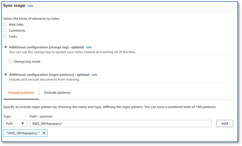
- On the Configure sync settings page, in the Sync scope section, you can include Box web links, comments, and tasks in your index, in addition to file contents. Use the default setting (unchecked) for this post.
- For Additional configuration (change log) – optional, use the default setting (unchecked).
- For Additional configuration (regex patterns) – optional, choose Include patterns.
- For Type, choose Path
- For Path – optional, enter the path to the sample documents you uploaded earlier:
AWS_Whitepapers/. - Choose Add.
- In the Sync run schedule section, choose Run on demand.
- Choose Next.

- On the Set fields mapping page, you can define how the data source maps attributes from Box objects to your index. Use the default settings for this post.
- Choose Next.
- On the Review and create page, review the details of your Box data source.
- To make changes, choose the Edit button next to the item that you want to change.
- When you’re done, choose Add data source to add your Box data source.
After you choose Add data source, Amazon Kendra starts creating the data source. It can take several minutes for the data source to be created. When it’s complete, the status of the data source changes from Creating to Active.
Index sample documents from the Box account
You configured the data source sync run schedule to run on demand, so you need to start it manually.
The current sync state changes to Syncing – crawling, then to Syncing – indexing.

After about 10 minutes, the current sync state changes to idle, the last sync status changes to Successful, and the Sync run history panel shows more details, including the number of documents added.

Test the solution
Now that you have ingested the AWS whitepapers from your Box account into your Amazon Kendra index, you can test some queries.
- On the Amazon Kendra console, choose Search indexed content in the navigation pane.

- In the query field, enter a test query, such as
What databases are offered by AWS?
You can try your own queries too.
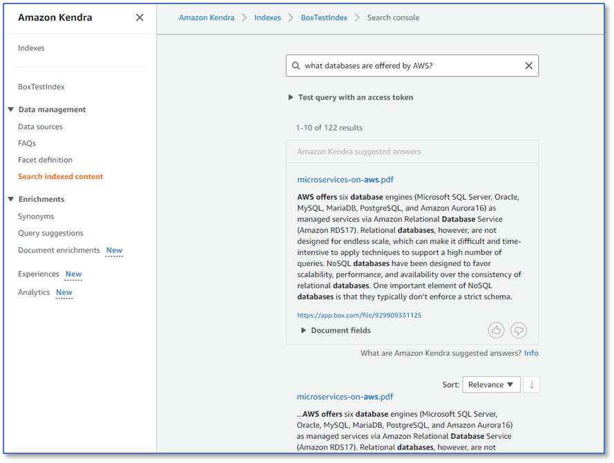
Congratulations! You have successfully used Amazon Kendra to surface answers and insights based on the content indexed from your Box account.
Clean up
To avoid incurring future costs, clean up the resources you created as part of this solution.
- If you created a new Amazon Kendra index while testing this solution, delete it.
- If you added a new data source using the Amazon Kendra connector for Box, delete that data source.
- Delete the
AWS_Whitepapersfolder and its contents from your Box account.
Conclusion
With the Amazon Kendra Box connector, organizations can make invaluable information trapped in their Box accounts available to their users securely using intelligent search powered by Amazon Kendra.
In this post, we introduced you to the basics, but there are many additional features that we didn’t cover. For example:
- You can enable user-based access control for your Amazon Kendra index, and restrict access to Box documents based on the access controls you have already configured in Box
- You can index additional Box object types, such as tasks, comments, and web links
- You can map Box object attributes to Amazon Kendra index attributes, and enable them for faceting, search, and display in the search results
- You can integrate the Box data source with the Custom Document Enrichment (CDE) capability in Amazon Kendra to perform additional attribute mapping logic and even custom content transformation during ingestion
To learn about these possibilities and more, refer to the Amazon Kendra Developer Guide.
About the Authors
 Bob Strahan is a Principal Solutions Architect in the AWS Language AI Services team.

