We introduce Flamingo, a single visual language model (VLM) that sets a new state of the art in few-shot learning on a wide range of open-ended multimodal tasks.Read More
Tackling multiple tasks with a single visual language model
We introduce Flamingo, a single visual language model (VLM) that sets a new state of the art in few-shot learning on a wide range of open-ended multimodal tasks.Read More
When a passion for bass and brass help build better tools
We caught up with Kevin Millikin, a software engineer on the DevTools team. He’s in Salt Lake City this week to present at PyCon US, the largest annual gathering for those using and developing the open-source Python programming language.Read More
Machine learning, harnessed to extreme computing, aids fusion energy development
MIT research scientists Pablo Rodriguez-Fernandez and Nathan Howard have just completed one of the most demanding calculations in fusion science — predicting the temperature and density profiles of a magnetically confined plasma via first-principles simulation of plasma turbulence. Solving this problem by brute force is beyond the capabilities of even the most advanced supercomputers. Instead, the researchers used an optimization methodology developed for machine learning to dramatically reduce the CPU time required while maintaining the accuracy of the solution.
Fusion energy
Fusion offers the promise of unlimited, carbon-free energy through the same physical process that powers the sun and the stars. It requires heating the fuel to temperatures above 100 million degrees, well above the point where the electrons are stripped from their atoms, creating a form of matter called plasma. On Earth, researchers use strong magnetic fields to isolate and insulate the hot plasma from ordinary matter. The stronger the magnetic field, the better the quality of the insulation that it provides.
Rodriguez-Fernandez and Howard have focused on predicting the performance expected in the SPARC device, a compact, high-magnetic-field fusion experiment, currently under construction by the MIT spin-out company Commonwealth Fusion Systems (CFS) and researchers from MIT’s Plasma Science and Fusion Center. While the calculation required an extraordinary amount of computer time, over 8 million CPU-hours, what was remarkable was not how much time was used, but how little, given the daunting computational challenge.
The computational challenge of fusion energy
Turbulence, which is the mechanism for most of the heat loss in a confined plasma, is one of the science’s grand challenges and the greatest problem remaining in classical physics. The equations that govern fusion plasmas are well known, but analytic solutions are not possible in the regimes of interest, where nonlinearities are important and solutions encompass an enormous range of spatial and temporal scales. Scientists resort to solving the equations by numerical simulation on computers. It is no accident that fusion researchers have been pioneers in computational physics for the last 50 years.
One of the fundamental problems for researchers is reliably predicting plasma temperature and density given only the magnetic field configuration and the externally applied input power. In confinement devices like SPARC, the external power and the heat input from the fusion process are lost through turbulence in the plasma. The turbulence itself is driven by the difference in the extremely high temperature of the plasma core and the relatively cool temperatures of the plasma edge (merely a few million degrees). Predicting the performance of a self-heated fusion plasma therefore requires a calculation of the power balance between the fusion power input and the losses due to turbulence.
These calculations generally start by assuming plasma temperature and density profiles at a particular location, then computing the heat transported locally by turbulence. However, a useful prediction requires a self-consistent calculation of the profiles across the entire plasma, which includes both the heat input and turbulent losses. Directly solving this problem is beyond the capabilities of any existing computer, so researchers have developed an approach that stitches the profiles together from a series of demanding but tractable local calculations. This method works, but since the heat and particle fluxes depend on multiple parameters, the calculations can be very slow to converge.
However, techniques emerging from the field of machine learning are well suited to optimize just such a calculation. Starting with a set of computationally intensive local calculations run with the full-physics, first-principles CGYRO code (provided by a team from General Atomics led by Jeff Candy) Rodriguez-Fernandez and Howard fit a surrogate mathematical model, which was used to explore and optimize a search within the parameter space. The results of the optimization were compared to the exact calculations at each optimum point, and the system was iterated to a desired level of accuracy. The researchers estimate that the technique reduced the number of runs of the CGYRO code by a factor of four.
New approach increases confidence in predictions
This work, described in a recent publication in the journal Nuclear Fusion, is the highest fidelity calculation ever made of the core of a fusion plasma. It refines and confirms predictions made with less demanding models. Professor Jonathan Citrin, of the Eindhoven University of Technology and leader of the fusion modeling group for DIFFER, the Dutch Institute for Fundamental Energy Research, commented: “The work significantly accelerates our capabilities in more routinely performing ultra-high-fidelity tokamak scenario prediction. This algorithm can help provide the ultimate validation test of machine design or scenario optimization carried out with faster, more reduced modeling, greatly increasing our confidence in the outcomes.”
In addition to increasing confidence in the fusion performance of the SPARC experiment, this technique provides a roadmap to check and calibrate reduced physics models, which run with a small fraction of the computational power. Such models, cross-checked against the results generated from turbulence simulations, will provide a reliable prediction before each SPARC discharge, helping to guide experimental campaigns and improving the scientific exploitation of the device. It can also be used to tweak and improve even simple data-driven models, which run extremely quickly, allowing researchers to sift through enormous parameter ranges to narrow down possible experiments or possible future machines.
The research was funded by CFS, with computational support from the National Energy Research Scientific Computing Center, a U.S. Department of Energy Office of Science User Facility.
MoLeR: Creating a path to more efficient drug design
Drug discovery has come a long way from its roots in serendipity. It is now an increasingly rational process, in which one important phase, called lead optimization, is the stepwise search for promising drug candidate compounds in the lab. In this phase, expert medicinal chemists work to improve “hit” molecules—compounds that demonstrate some promising properties, as well as some undesirable ones, in early screening. In subsequent testing, chemists try to adapt the structure of hit molecules to improve their biological efficacy and reduce potential side effects. This process combines knowledge, creativity, experience, and intuition, and often lasts for years. Over many decades, computational modelling techniques have been developed to help predict how the molecules will fare in the lab, so that costly and time-consuming experiments can focus on the most promising compounds.

The Microsoft Generative Chemistry team is working with Novartis to improve these modelling techniques with a new model called MoLeR.
“MoLeR illustrates how generative models based on deep learning can help transform the drug discovery process and enable our colleagues at Novartis to increase the efficiency in finding new compounds.”
Christopher Bishop, Technical Fellow and Laboratory Director, Microsoft Research Cambridge
We recently focused on predicting molecular properties using machine learning methods in the FS-Mol project. To further support the drug discovery process, we are also working on methods that can automatically design compounds that better fit project requirements than existing candidate compounds. This is an extremely difficult task, as only a few promising molecules exist in the vast and largely unexplored chemical space—estimated to contain up to 1060 drug-like molecules. Just how big is that number? It would be enough molecules to reproduce the Earth billions of times. Finding them requires creativity and intuition that cannot be captured by fixed rules or hand-designed algorithms. This is why learning is crucial not only for the predictive task, as done in FS-Mol, but also for the generative task of coming up with new structures.
In our earlier work, published at the 2018 Conference on Neural Information Processing Systems (NeurIPS), we described a generative model of molecules called CGVAE. While that model performed well on simple, synthetic tasks, we noted then that further improvements required the expertise of drug discovery specialists. In collaboration with experts at Novartis, we identified two issues limiting the applicability of the CGVAE model in real drug discovery projects: it cannot be naturally constrained to explore only molecules containing a particular substructure (called the scaffold), and it struggles to reproduce key structures, such as complex ring systems, due to its low-level, atom-by-atom generative procedure. To remove these limitations, we built MoLeR, which we describe in our new paper, “Learning to Extend Molecular Scaffolds with Structural Motifs,” published at the 2022 International Conference on Learning Representations (ICLR).
The MoLeR model
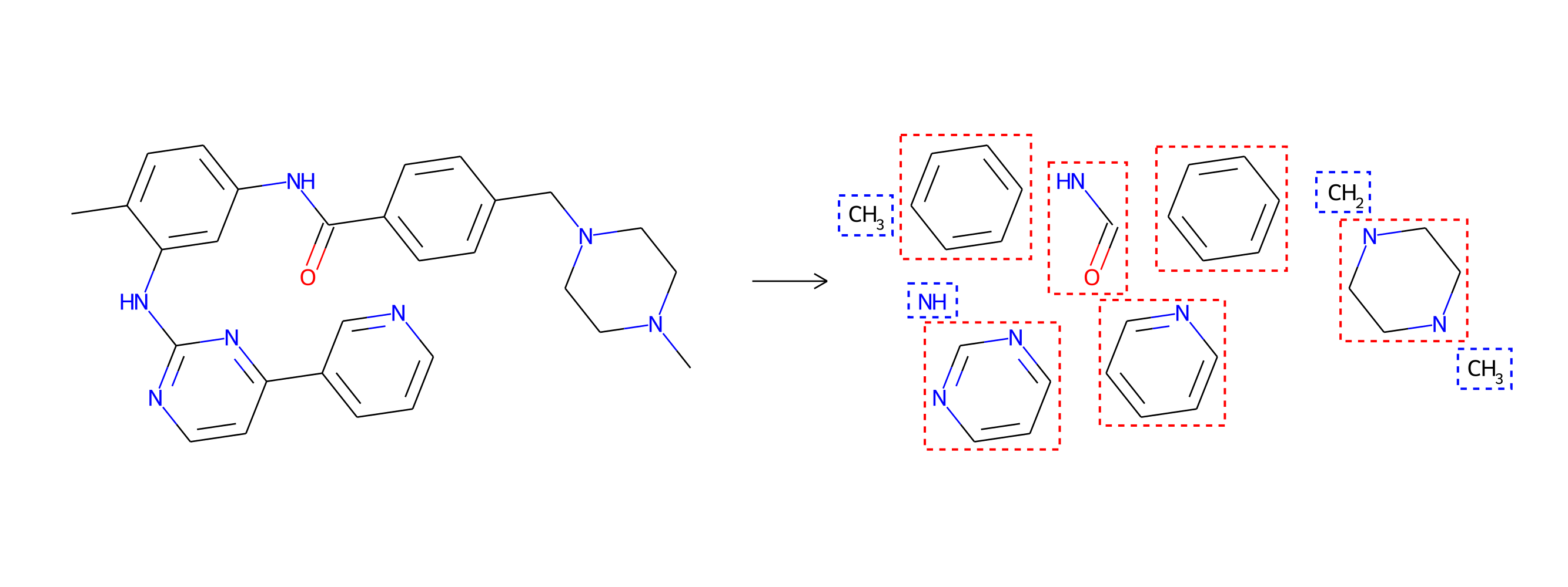
In the MoLeR model, we represent molecules as graphs, in which atoms appear as vertices that are connected by edges corresponding to the bonds. Our model is trained in the auto-encoder paradigm, meaning that it consists of an encoder—a graph neural network (GNN) that aims to compress an input molecule into a so-called latent code—and a decoder, which tries to reconstruct the original molecule from this code. As the decoder needs to decompress a short encoding into a graph of arbitrary size, we design the reconstruction process to be sequential. In each step, we extend a partially generated graph by adding new atoms or bonds. A crucial feature of our model is that the decoder makes predictions at each step solely based on a partial graph and a latent code, rather than in dependence on earlier predictions. We also train MoLeR to construct the same molecule in a variety of different orders, as the construction order is an arbitrary choice.

As we alluded to earlier, drug molecules are not random combinations of atoms. They tend to be composed of larger structural motifs, much like sentences in a natural language are compositions of words, and not random sequences of letters. Thus, unlike CGVAE, MoLeR first discovers these common building blocks from data, and is then trained to extend a partial molecule using entire motifs (rather than single atoms). Consequently, MoLeR not only needs fewer steps to construct drug-like molecules, but its generation procedure also occurs in steps that are more akin to the way chemists think about the construction of molecules.
Drug-discovery projects often focus on a specific subset of the chemical space, by first defining a scaffold—a central part of the molecule that has already shown promising properties—and then exploring only those compounds that contain the scaffold as a subgraph. The design of MoLeR’s decoder allows us to seamlessly integrate an arbitrary scaffold by using it as an initial state in the decoding loop. As we randomize the generation order during training, MoLeR implicitly learns to complete arbitrary subgraphs, making it ideal for focused scaffold-based exploration.
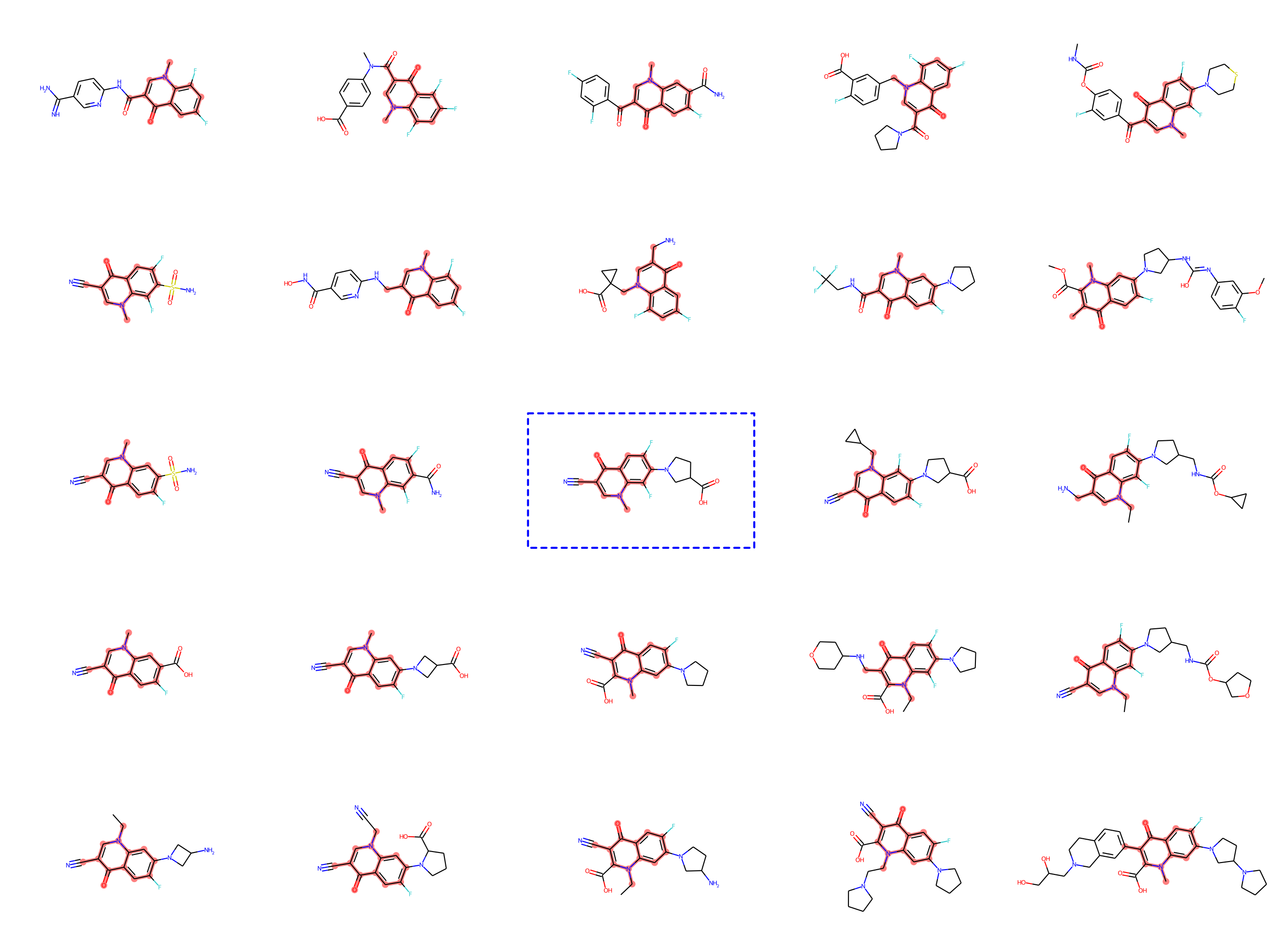
Optimization with MoLeR
Even after training our model as discussed above, MoLeR has no notion of “optimization” of molecules. However, like related approaches, we can perform optimization in the space of latent codes using an off-the-shelf black-box optimization algorithm. This was not possible with CGVAE, which used a much more complicated encoding of graphs. In our work, we opted for using Molecular Swarm Optimization (MSO), which shows state-of-the-art results for latent space optimization in other models, and indeed we found it to work very well for MoLeR. In particular, we evaluated optimization with MSO and MoLeR on new benchmark tasks that are similar to realistic drug discovery projects using large scaffolds and found this combination to outperform existing models.
Outlook
We continue to work with Novartis to focus machine learning research on problems relevant to the real-world drug discovery process. The early results are substantially better than those of competing methods, including our earlier CGVAE model. With time, we hope MoLeR-generated compounds will reach the final stages of drug-discovery projects, eventually contributing to new useful drugs that benefit humanity.
The post MoLeR: Creating a path to more efficient drug design appeared first on Microsoft Research.
Registration remains open for June Amazon re:MARS event
Event’s speaker roster expands for keynotes, innovation spotlights, and leadership sessions.Read More
Answers Blowin’ in the Wind: HPC Code Gives Renewable Energy a Lift
A hundred and forty turbines in the North Sea — and some GPUs in the cloud — pumped wind under the wings of David Standingford and Jamil Appa’s dream.
As colleagues at a British aerospace firm, they shared a vision of starting a company to apply their expertise in high performance computing across many industries.
They formed Zenotech and coded what they learned about computational fluid dynamics into a program called zCFD. They also built a tool, EPIC, that simplified running it and other HPC jobs on the latest hardware in public clouds.
But getting visibility beyond their Bristol, U.K. home was a challenge, given the lack of large, open datasets to show what their tools could do.
Harvesting a Wind Farm’s Data
Their problem dovetailed with one in the wind energy sector.
As government subsidies for wind farms declined, investors demanded a deeper analysis of a project’s likely return on investment, something traditional tools didn’t deliver. A U.K. government project teamed Zenotech with consulting firms in renewable energy and SSE, a large British utility willing to share data on its North Sea wind farm, one of the largest in the world.
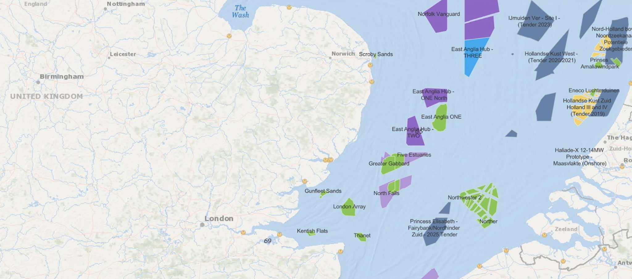
Using zCFD, Zenotech simulated the likely energy output of the farm’s 140 turbines. The program accounted for dozens of wind speeds and directions. This included key but previously untracked phenomena in front of and behind a turbine, like the combined effects the turbines had on each other.
“These so-called ‘wake’ and ‘blockage’ effects around a wind farm can even impact atmospheric currents,” said Standingford, a director and co-founder of Zenotech.
The program can also track small but significant terrain effects on the wind, such as when trees in a nearby forest lose their leaves.
SSE validated that the final simulation came within 2 percent of the utility’s measured data, giving zCFD a stellar reference.
Accelerated in the Cloud
Icing the cake, Zenotech showed cloud GPUs delivered results fast and cost effectively.
For example, the program ran 43x faster on NVIDIA A100 Tensor Core GPUs than CPUs at a quarter of the CPUs’ costs, the company reported in a recent GTC session (viewable on-demand). NVIDIA NCCL libraries that speed communications between GPU systems further boosted results up to 15 percent.

As a result, work that took more than five hours on CPUs ran in less than 50 minutes on GPUs. The ability to analyze nuanced wind effects in detail and finish a report in a day “got people’s attention,” Standingford said.
“The tools and computing power to perform high-fidelity simulations of wind projects are now affordable and accessible to the wider industry,” he concluded in a report on the project.
Lowering Carbon, Easing Climate Change
Wind energy is among the largest, most cost-effective contributors to lowering carbon emissions, notes Farah Hariri, technical lead for the team helping NVIDIA’s customers manage their transitions to net-zero emissions.
“By modeling both wake interactions and the blockage effects, zCFD helps wind farms extract the maximum energy for the minimum installation costs,” she said.
This kind of fast yet detailed analysis lowers risk for investors, making wind farms more economically attractive than traditional energy sources, said Richard Whiting, a partner at Everose, one of the consultants who worked on the project with Zenotech.
Looking forward, Whiting estimates more than 2,100 gigawatts of wind farms could be in operation worldwide by 2030, up 3x from in 2020. It’s a growing opportunity on many levels.
“In future, we expect projects will use larger arrays of larger turbines so the modeling challenge will only get bigger,” he added.
Less Climate Change, More Business
Helping renewable projects get off the ground also put wind in Zenotech’s sails.
Since the SSE analysis, the company has helped design wind farms or turbines in at least 10 other projects across Europe and Asia. And half of Zenotech’s business is now outside the U.K.
As the company expands, it’s also revisiting its roots in aerospace, lifting the prospects of new kinds of businesses for drones and air taxis.
A Parallel Opportunity
For example, Cardiff Airport is sponsoring live trials where emerging companies use zCFD on cloud GPUs to predict wind shifts in urban environments so they can map safe, efficient routes.
“It’s a forward-thinking way to use today’s managed airspace to plan future services like air taxis and automated airport inspections,” said Standingford.
“We’re seeing a lot of innovation in small aircraft platforms, and we’re working with top platform makers and key sites in the U.K.”
It’s one more way the company is keeping its finger to the wind.
The post Answers Blowin’ in the Wind: HPC Code Gives Renewable Energy a Lift appeared first on NVIDIA Blog.
What Is Conversational AI? ZeroShot Bot CEO Jason Mars Explains
Entrepreneur Jason Mars calls conversation our “first technology.”
Before humans invented the wheel, crafted a spear or tamed fire, we mastered the superpower of talking to one another.
That makes conversation an incredibly important tool.
But if you’ve dealt with the automated chatbots deployed by the customer service arms of just about any big organization lately — whether banks or airlines — you also know how hard it can be to get it right.
Deep learning AI and new techniques such as zero-shot learning promise to change that.
On this episode of NVIDIA’s AI Podcast, host Noah Kravitz — whose intelligence is anything but artificial — spoke with Mars about how the latest AI techniques intersect with the very ancient art of conversation.
In addition to being an entrepreneur and CEO of several startups, including Zero Shot Bot, Mars is an associate professor of computer science at the University of Michigan and the author of “Breaking Bots: Inventing a New Voice in the AI Revolution” (ForbesBooks, 2021).
You Might Also Like
NVIDIA’s Liila Torabi Talks the New Era of Robotics Through Isaac Sim
Robots aren’t limited to the assembly line. Liila Torabi, senior product manager for Isaac Sim, a robotics and AI simulation platform powered by NVIDIA Omniverse, talks about where the field’s headed.
GANTheftAuto: Harrison Kinsley on AI-Generated Gaming Environments
Humans playing games against machines is nothing new, but now computers can develop their own games for people to play. Programming enthusiast and social media influencer Harrison Kinsley created GANTheftAuto, an AI-based neural network that generates a playable chunk of the classic video game Grand Theft Auto V.
The Driving Force: How Ford Uses AI to Create Diverse Driving Data
The neural networks powering autonomous vehicles require petabytes of driving data to learn how to operate. Nikita Jaipuria and Rohan Bhasin from Ford Motor Company explain how they use generative adversarial networks (GANs) to fill in the gaps of real-world data used in AV training.
Subscribe to the AI Podcast: Now available on Amazon Music
You can now listen to the AI Podcast through Amazon Music.
You can also get the AI Podcast through iTunes, Google Podcasts, Google Play, Castbox, DoggCatcher, Overcast, PlayerFM, Pocket Casts, Podbay, PodBean, PodCruncher, PodKicker, Soundcloud, Spotify, Stitcher and TuneIn.
Make the AI Podcast Better: Have a few minutes to spare? Fill out our listener survey.
The post What Is Conversational AI? ZeroShot Bot CEO Jason Mars Explains appeared first on NVIDIA Blog.
Build and deploy a scalable machine learning system on Kubernetes with Kubeflow on AWS
In this post, we demonstrate Kubeflow on AWS (an AWS-specific distribution of Kubeflow) and the value it adds over open-source Kubeflow through the integration of highly optimized, cloud-native, enterprise-ready AWS services.
Kubeflow is the open-source machine learning (ML) platform dedicated to making deployments of ML workflows on Kubernetes simple, portable and scalable. Kubeflow provides many components, including a central dashboard, multi-user Jupyter notebooks, Kubeflow Pipelines, KFServing, and Katib, as well as distributed training operators for TensorFlow, PyTorch, MXNet, and XGBoost, to build simple, scalable, and portable ML workflows.
AWS recently launched Kubeflow v1.4 as part of its own Kubeflow distribution (called Kubeflow on AWS), which streamlines data science tasks and helps build highly reliable, secure, portable, and scalable ML systems with reduced operational overheads through integrations with AWS managed services. You can use this Kubeflow distribution to build ML systems on top of Amazon Elastic Kubernetes Service (Amazon EKS) to build, train, tune, and deploy ML models for a wide variety of use cases, including computer vision, natural language processing, speech translation, and financial modeling.
Challenges with open-source Kubeflow
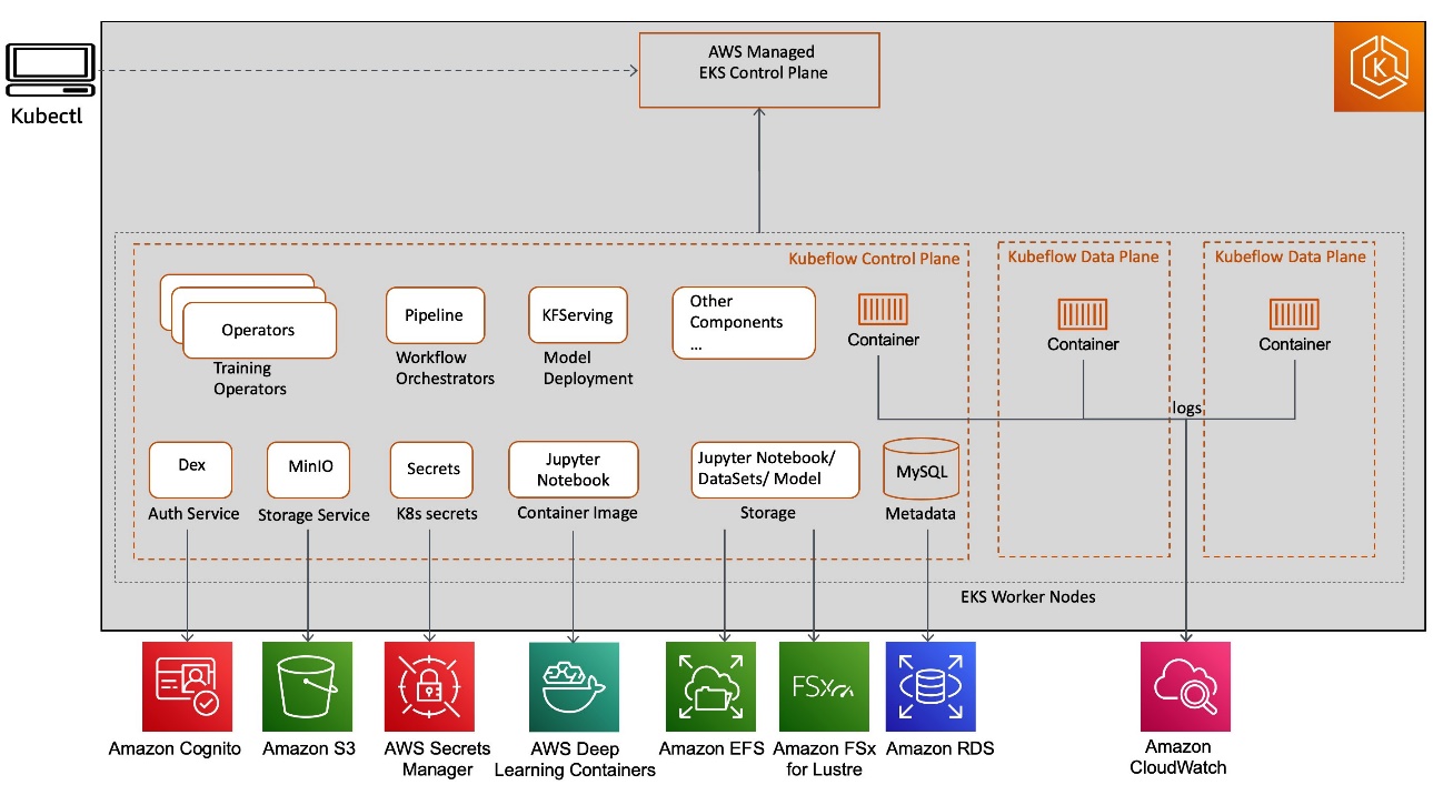
When you use an open-source Kubeflow project, it deploys all Kubeflow control plane and data plane components on Kubernetes worker nodes. Kubeflow component services are deployed as part of the Kubeflow control plane, and all resource deployments related to Jupyter, model training, tuning, and hosting are deployed on the Kubeflow data plane. The Kubeflow control plane and data plane can run on the same or different Kubernetes worker nodes. This post focuses on Kubeflow control plane components, as illustrated in the following diagram.
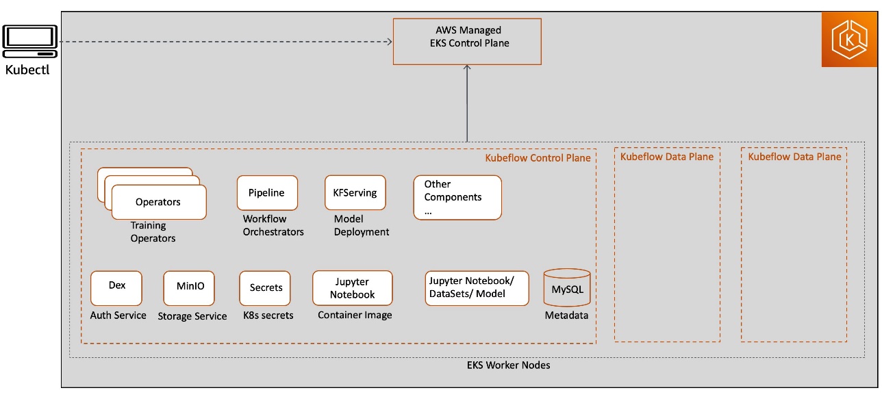
This deployment model may not provide an enterprise-ready experience due to the following reasons:
- All Kubeflow control plane heavy lifting infrastructure components, including database, storage, and authentication, are deployed in the Kubernetes cluster worker node itself. This makes it challenging to implement a highly available Kubeflow control plane design architecture with a persistent state in the event of worker node failure.
- Kubeflow control plane generated artifacts (such as MySQL instances, pod logs, or MinIO storage) grow over time and need resizable storage volumes with continuous monitoring capabilities to meet the growing storage demand. Because the Kubeflow control plane shares resources with Kubeflow data plane workloads (for example, for training jobs, pipelines, and deployments), right-sizing and scaling Kubernetes cluster and storage volumes can become challenging and result in increased operational cost.
- Kubernetes restricts the log file size, with most installations keeping the most recent limit of 10 MB. By default, the pod logs become inaccessible after they reach this upper limit. The logs could also become inaccessible if pods are evicted, crashed, deleted, or scheduled on a different node, which could impact your application log availability and monitoring capabilities.
Kubeflow on AWS
Kubeflow on AWS provides a clear path to use Kubeflow, with the following AWS services:
- Application Load Balancer for secure external traffic management over HTTPS
- Amazon CloudWatch for persistent log management
- AWS Cognito for user authentication with Transport Layer Security (TLS)
- AWS Deep Learning Containers for highly optimized Jupyter notebook server images
- Amazon Elastic File System (Amazon EFS) or Amazon FSx for Lustre for a simple, scalable, and serverless file storage solution for increased training performance
- Amazon EKS for managed Kubernetes clusters
- Amazon Relational Database Service (Amazon RDS) for highly scalable pipelines and a metadata store
- AWS Secrets Manager to protect secrets needed to access your applications
- Amazon Simple Storage Service (Amazon S3) for an easy-to-use pipeline artifacts store
These AWS service integrations with Kubeflow (as shown in the following diagram) allow us to decouple critical parts of the Kubeflow control plane from Kubernetes, providing a secure, scalable, resilient, and cost-optimized design.
Let’s discuss the benefits of each service integration and their solutions around security, running ML pipelines, and storage.
Secure authentication of Kubeflow users with Amazon Cognito
Cloud security at AWS is the highest priority, and we’re investing in tightly integrating Kubeflow security directly into the AWS shared-responsibility security services, such as the following:
- Application Load Balancer (ALB) for external traffic management
- AWS Certificate Manager (ACM) to support TLS
- IAM roles for service accounts (IRSA) for fine-grained access control at the Kubernetes Pod level
- AWS Key Management Service (AWS KMS) for data encryption key management
- AWS Shield for DDoS protection
In this section, we focus on AWS Kubeflow control plane integration with Amazon Cognito. Amazon Cognito removes the need to manage and maintain a native Dex (open-source OpenID Connect (OIDC) provider backed by local LDAP) solution for user authentication and makes secret management easier.
You can also use Amazon Cognito to add user sign-up, sign-in, and access control to your Kubeflow UI quickly and easily. Amazon Cognito scales to millions of users and supports sign-in with social identity providers (IdPs), such as Facebook, Google, and Amazon, and enterprise IdPs via SAML 2.0. This reduces the complexity in your Kubeflow setup, making it operationally lean and easier to operate to achieve multi-user isolation.
Let’s look at a multi-user authentication flow with Amazon Cognito, ALB, and ACM integrations with Kubeflow on AWS. There are a number of key components as part of this integration. Amazon Cognito is configured as an IdP with an authentication callback configured to route the request to Kubeflow after user authentication. As part of the Kubeflow setup, a Kubernetes ingress resource is created to manage external traffic to the Istio Gateway service. The AWS ALB Ingress Controller provisions a load balancer for that ingress. We use Amazon Route 53 to configure a public DNS for the registered domain and create certificates using ACM to enable TLS authentication at the load balancer.
The following diagram shows the typical user workflow of logging in to Amazon Cognito and getting redirected to Kubeflow in their respective namespace.
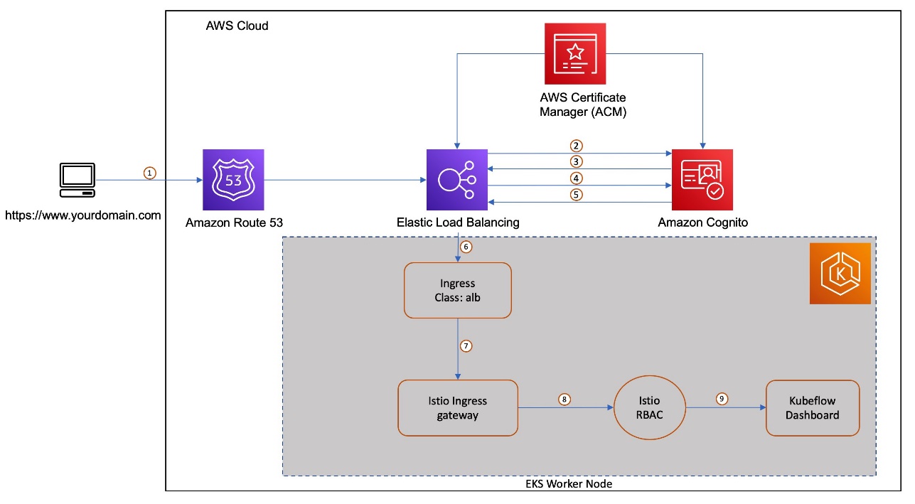
The workflow contains the following steps:
- The user sends an HTTPS request to the Kubeflow central dashboard hosted behind a load balancer. Route 53 resolves the FQDN to the ALB alias record.
- If the cookie isn’t present, the load balancer redirects the user to the Amazon Cognito authorization endpoint so that Amazon Cognito can authenticate the user.
- After the user is authenticated, Amazon Cognito sends the user back to the load balancer with an authorization grant code.
- The load balancer presents the authorization grant code to the Amazon Cognito token endpoint.
- Upon receiving a valid authorization grant code, Amazon Cognito provides the ID token and access token to load balancer.
- After your load balancer authenticates a user successfully, it sends the access token to the Amazon Cognito user info endpoint and receives user claims. The load balancer signs and adds user claims to the HTTP header
x-amzn-oidc-*in a JSON web token (JWT) request format. - The request from the load balancer is sent to the Istio Ingress Gateway’s pod.
- Using an envoy filter, Istio Gateway decodes the
x-amzn-oidc-datavalue, retrieves the email field, and adds the custom HTTP headerkubeflow-userid, which is used by the Kubeflow authorization layer. - The Istio resource-based access control policies are applied to the incoming request to validate the access to the Kubeflow Dashboard. If either of those are inaccessible to the user, an error response is sent back. If the request is validated, it’s forwarded to the appropriate Kubeflow service and provides access to the Kubeflow Dashboard
Persisting Kubeflow component metadata and artifact storage with Amazon RDS and Amazon S3
Kubeflow on AWS provides integration with Amazon Relational Database Service (Amazon RDS) in Kubeflow Pipelines and AutoML (Katib) for persistent metadata storage, and Amazon S3 in Kubeflow Pipelines for persistent artifact storage. Let’s continue to discuss Kubeflow Pipelines in more detail.
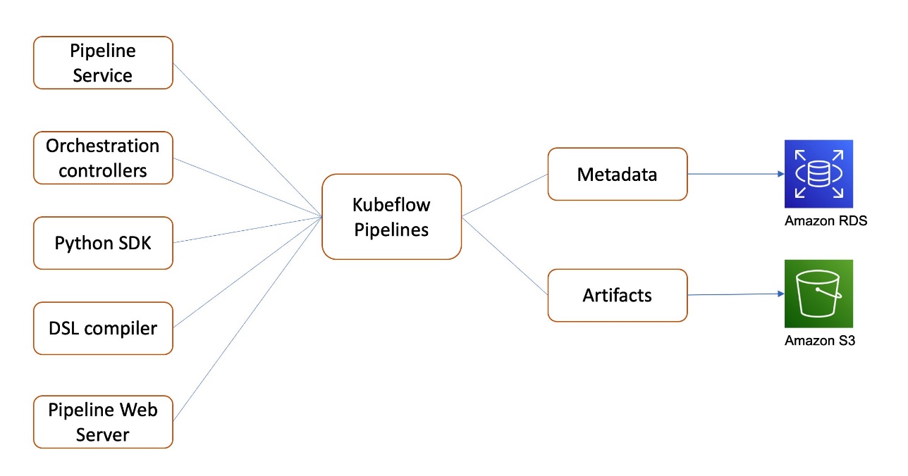
Kubeflow Pipelines is a platform for building and deploying portable, scalable ML workflows. These workflows can help automate complex ML pipelines using built-in and custom Kubeflow components. Kubeflow Pipelines includes Python SDK, a DSL compiler to convert Python code into a static config, a Pipelines service that runs pipelines from the static configuration, and a set of controllers to run the containers within the Kubernetes Pods needed to complete the pipeline.
Kubeflow Pipelines metadata for pipeline experiments and runs are stored in MySQL, and artifacts including pipeline packages and metrics are stored in MinIO.
As shown in the following diagram, Kubeflow on AWS lets you store the following components with AWS managed services:
- Pipeline metadata in Amazon RDS – Amazon RDS provides a scalable, highly available, and reliable Multi-AZ deployment architecture with a built-in automated failover mechanism and resizable capacity for an industry-standard relational database like MySQL. It manages common database administration tasks without needing to provision infrastructure or maintain software.
- Pipeline artifacts in Amazon S3 – Amazon S3 offers industry-leading scalability, data availability, security, and performance, and could be used to meet your compliance requirements.
These integrations help offload the management and maintenance of the metadata and artifact storage from self-managed Kubeflow to AWS managed services, which is easier to set up, operate, and scale.
Support for distributed file systems with Amazon EFS and Amazon FSx
Kubeflow builds upon Kubernetes, which provides an infrastructure for large-scale, distributed data processing, including training and tuning large models with a deep network with millions or even billions of parameters. To support such distributed data processing ML systems, Kubeflow on AWS provides integration with the following storage services:
-
Amazon EFS – A high-performance, cloud-native, distributed file system, which you could manage through an Amazon EFS CSI driver. Amazon EFS provides
ReadWriteManyaccess mode, and you can now use it to mount into pods (Jupyter, model training, model tuning) running in a Kubeflow data plane to provide a persistent, scalable, and shareable workspace that automatically grows and shrinks as you add and remove files with no need for management. -
Amazon FSx for Lustre – An optimized file system for compute-intensive workloads, such as high-performance computing and ML, that you can manage through the Amazon FSx CSI driver. FSx for Lustre provides
ReadWriteManyaccess mode as well, and you can use it to cache training data with direct connectivity to Amazon S3 as the backing store, which you can use to support Jupyter notebook servers or distributed training running in a Kubeflow data plane. With this configuration, you don’t need to transfer data to the file system before using the volume. FSx for Lustre provides consistent submillisecond latencies and high concurrency, and can scale to TB/s of throughput and millions of IOPS.
Kubeflow deployment options
AWS provides various Kubeflow deployment options:
- Deployment with Amazon Cognito
- Deployment with Amazon RDS and Amazon S3
- Deployment with Amazon Cognito, Amazon RDS, and Amazon S3
- Vanilla deployment
For details on service integration and available add-ons for each of these options, refer to Deployment Options. You can fit the option that best fits your use case.
In the following section, we walk through the steps to install AWS Kubeflow v1.4 distribution on Amazon EKS. Then we use the existing XGBoost pipeline example available on the Kubeflow central UI dashboard to demonstrate the integration and usage of AWS Kubeflow with Amazon Cognito, Amazon RDS, and Amazon S3, with Secrets Manager as an add-on.
Prerequisites
For this walkthrough, you should have the following prerequisites:
- An AWS account.
- An existing Amazon EKS cluster. It should be Kubernetes version 1.19 or higher. For automated cluster creation using eksctl, see Create an Amazon EKS Cluster and use the eksctl option.
Install the following tools on the client machine used to access your Kubernetes cluster. You can use AWS Cloud9, a cloud-based integrated development environment (IDE) for the Kubernetes cluster setup.
- AWS Command Line Interface (AWS CLI) – A command line tool for interacting with AWS services. For installation instructions, refer to Installing, updating, and uninstalling the AWS CLI.
- eksctl > 0.56 – A command line tool for working with Amazon EKS clusters that automates many individual tasks.
- kubectl – A command line tool for working with Kubernetes clusters.
- git – A distributed version control software.
- Python 3.8+ – The Python programming environment.
- pip – The package manager for Python.
- kustomize version 3.2.0 – A command line tool to customize Kubernetes objects through a kustomization file.
Install Kubeflow on AWS
Configure kubectl so that you can connect to an Amazon EKS cluster:
Various controllers in Kubeflow deployment use IAM roles for service accounts (IRSA). An OIDC provider must exist for your cluster to use IRSA. Create an OIDC provider and associate it with for your Amazon EKS cluster by running the following command, if your cluster doesn’t already have one:
Clone the AWS manifests repo and Kubeflow manifests repo, and checkout the respective release branches:
For more information about these versions, refer to Releases and Versioning.
Set up Amazon RDS, Amazon S3, and Secrets Manager
You create Amazon RDS and Amazon S3 resources before you deploy the Kubeflow manifests. We use automated Python scripts that take care of creating the S3 bucket, RDS database, and required secrets in Secrets Manager. It also edits the required configuration files for the Kubeflow pipeline and AutoML to be properly configured for the RDS database and S3 bucket during Kubeflow installation.
Create an IAM user with permissions to allow GetBucketLocation and read and write access to objects in an S3 bucket where you want to store the Kubeflow artifacts. Use the AWS_ACCESS_KEY_ID and AWS_SECRET_ACCESS_KEY of the IAM user in the following code:
Set up Amazon Cognito as the authentication provider
In this section, we create a custom domain in Route 53 and ALB to route external traffic to Kubeflow Istio Gateway. We use ACM to create a certificate to enable TLS authentication at ALB and Amazon Cognito to maintain the user pool and manage user authentication.
Substitute the following values in
-
route53.rootDomain.name – The registered domain. Let’s assume this domain is
example.com. - route53.rootDomain.hostedZoneId – If your domain is managed in Route53, enter the hosted zone ID found under the hosted zone details. Skip this step if your domain is managed by another domain provider.
-
route53.subDomain.name – The name of the subdomain where you want to host Kubeflow (for example,
platform.example.com). For more information about subdomains, refer to Deploying Kubeflow with AWS Cognito as IdP. - cluster.name – The cluster name and where Kubeflow is deployed.
-
cluster.region – The cluster Region where Kubeflow is deployed (for example,
us-west-2). -
cognitoUserpool.name – The name of the Amazon Cognito user pool (for example,
kubeflow-users).
The config file looks something like the following code:
Run the script to create the resources:
The script updates the config.yaml file with the resource names, IDs, and ARNs it created. It looks something like the following code:
Build manifests and deploy Kubeflow
Deploy Kubeflow using the following command:
Update the domain with the ALB address
The deployment creates an ingress-managed AWS application load balancer. We update the DNS entries for the subdomain in Route 53 with the DNS of the load balancer. Run the following command to check if the load balancer is provisioned (this takes around 3–5 minutes):
If the ADDRESS field is empty after a few minutes, check the logs of alb-ingress-controller. For instructions, refer to ALB fails to provision.
When the load balancer is provisioned, copy the DNS name of the load balancer and substitute the address for kubeflow.alb.dns in ${kubeflow_manifest_dir}/tests/e2e/utils/cognito_bootstrap/config.yaml. The Kubeflow section of the config file looks like the following code:
Run the following script to update the DNS entries for the subdomain in Route 53 with the DNS of the provisioned load balancer:
Troubleshooting
If you run into any issues during the installation, refer to the troubleshooting guide or start fresh by following the “Clean up” section in this blog.
Use case walkthrough
Now that we have completed installing the required Kubeflow components, let’s see them in action using one of the existing examples provided by Kubeflow Pipelines on the dashboard.
Access the Kubeflow Dashboard using Amazon Cognito
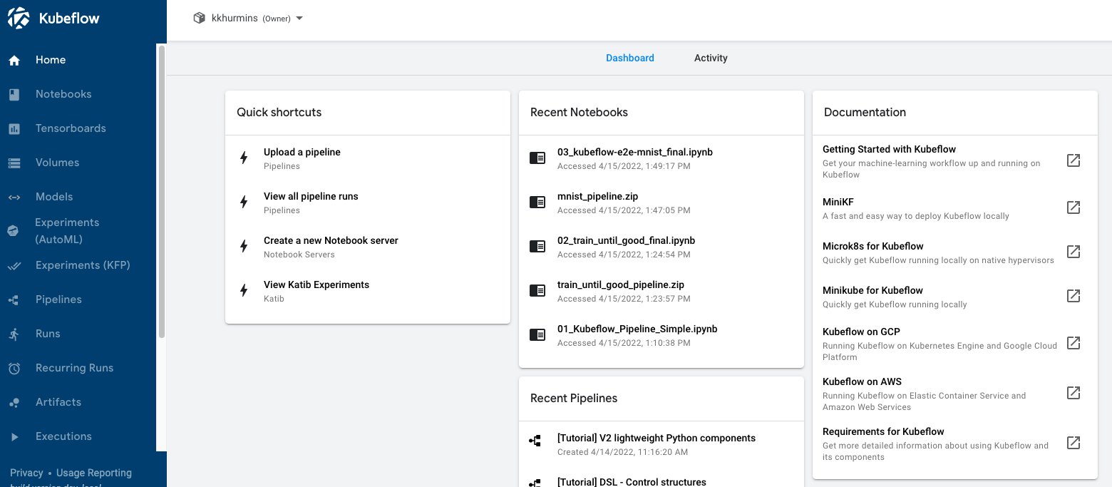
To get started, let’s get access to the Kubeflow Dashboard. Because we used Amazon Cognito as the IdP, use the information provided in the official README file. We first create some users on the Amazon Cognito console. These are the users who will log in to the central dashboard. Next, create a profile for the user you created. Then you should be able to access the dashboard through the login page at https://kubeflow.platform.example.com.
The following screenshot shows our Kubeflow Dashboard.
Run the pipeline
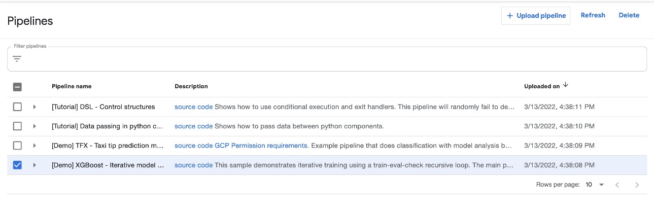
On the Kubeflow Dashboard, choose Pipelines in the navigation name. You should see four examples provided by Kubeflow Pipelines that you can run directly to explore various Pipelines features.
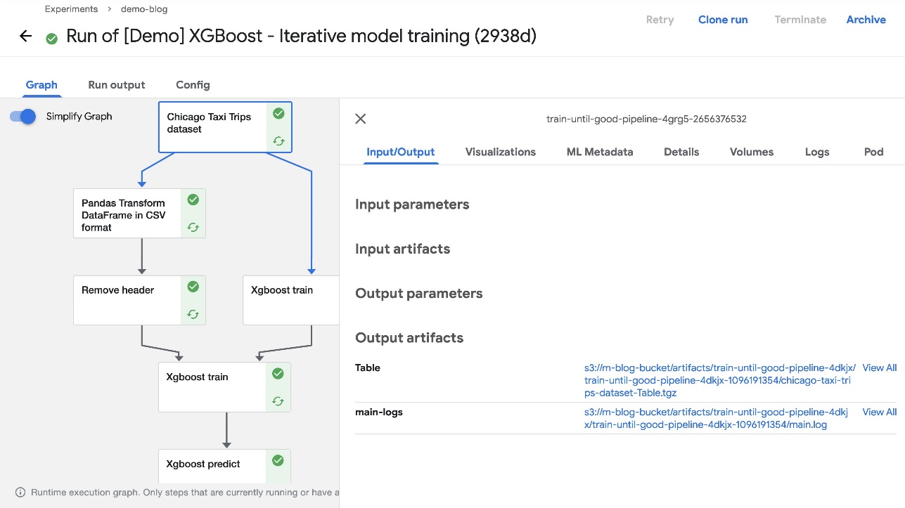
For this post, we use the XGBoost sample called [Demo] XGBoost – Iterative model training. You can find the source code on GitHub. This is a simple pipeline that uses the existing XGBoost/Train and XGBoost/Predict Kubeflow pipeline components to iteratively train a model until the metrics are considered good based on specified metrics.
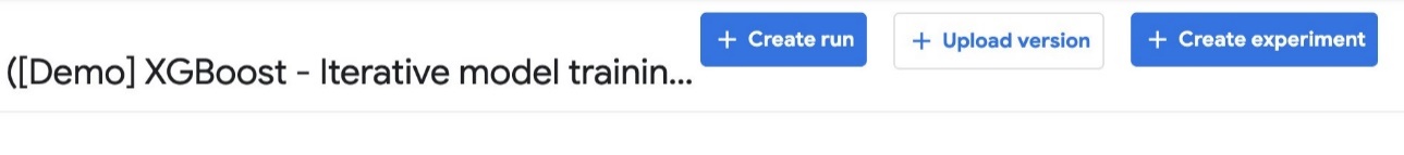
To run the pipeline, complete the following steps:
- Select the pipeline and choose Create experiment.
- Under Experiment details, enter a name (for this post,
demo-blog) and optional description. - Choose Next.

- Under Run details¸ choose your pipeline and pipeline version.
- For Run name, enter a name.
- For Experiment, choose the experiment you created.
- For Run type, select One-off.
- Choose Start.

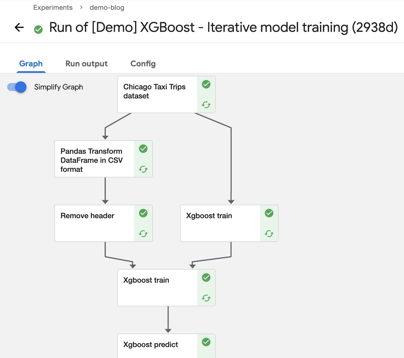
After the pipeline starts running, you should see components completing (within a few seconds). At this stage, you can choose any of the completed components to see more details.
Access the artifacts in Amazon S3
While deploying Kubeflow, we specified Kubeflow Pipelines should use Amazon S3 to store its artifacts. This includes all pipeline output artifacts, cached runs, and pipeline graphs—all of which can then be used for rich visualizations and performance evaluation.
When the pipeline run is complete, you should be able to see the artifacts in the S3 bucket you created during installation. To confirm this, choose any completed component of the pipeline and check the Input/Output section on the default Graph tab. The artifact URLs should point to the S3 bucket that you specified during deployment.
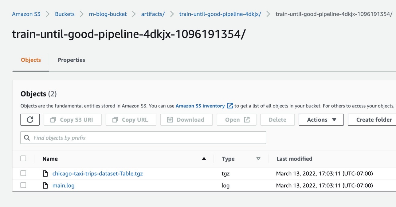
To confirm that the resources were added to Amazon S3, we can also check the S3 bucket in our AWS account via the Amazon S3 console.
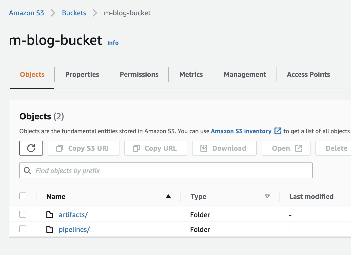
The following screenshot shows our files.
Verify ML metadata in Amazon RDS
We also integrated Kubeflow Pipelines with Amazon RDS during deployment, which means that any pipeline metadata should be stored in Amazon RDS. This includes any runtime information such as the status of a task, availability of artifacts, custom properties associated with the run or artifacts, and more.
To verify the Amazon RDS integration, follow the steps provided in the official README file. Specifically, complete the following steps:
- Get the Amazon RDS user name and password from the secret that was created during the installation:
- Use these credentials to connect to Amazon RDS from within the cluster:
- When the MySQL prompt opens, we can verify the
mlpipelinesdatabase as follows: - Now we can read the content of specific tables, to make sure that we can see metadata information about the experiments that ran the pipelines:
Clean up
To uninstall Kubeflow and delete the AWS resources you created, complete the following steps:
- Delete the ingress and ingress-managed load balancer by running the following command:
- Delete the rest of the Kubeflow components:
- Delete the AWS resources created by scripts:
- Resources created for Amazon RDS and Amazon S3 integration. Make sure you have the configuration file created by the script in
${kubeflow_manifest_dir}/tests/e2e/utils/rds-s3/metadata.yaml: - Resources created for Amazon Cognito integration. Make sure you have the configuration file created by the script in
${kubeflow_manifest_dir}/tests/e2e/utils/cognito_bootstrap/config.yaml:
- Resources created for Amazon RDS and Amazon S3 integration. Make sure you have the configuration file created by the script in
- If you created a dedicated Amazon EKS cluster for Kubeflow using eksctl, you can delete it with the following command:
Summary
In this post, we highlighted the value that Kubeflow on AWS provides through native AWS-managed service integrations for secure, scalable, and enterprise-ready AI and ML workloads. You can choose from several deployment options to install Kubeflow on AWS with various service integrations. The use case in this post demonstrated Kubeflow integration with Amazon Cognito, Secrets Manager, Amazon RDS, and Amazon S3. To get started with Kubeflow on AWS, refer to the available AWS-integrated deployment options in Kubeflow on AWS.
Starting with v1.3, you can follow the AWS Labs repository to track all AWS contributions to Kubeflow. You can also find us on the Kubeflow #AWS Slack Channel; your feedback there will help us prioritize the next features to contribute to the Kubeflow project.
About the Authors
 Kanwaljit Khurmi is an AI/ML Specialist Solutions Architect at Amazon Web Services. He works with the AWS product, engineering and customers to provide guidance and technical assistance helping them improve the value of their hybrid ML solutions when using AWS. Kanwaljit specializes in helping customers with containerized and machine learning applications.
 Meghna Baijal is a Software Engineer with AWS AI making it easier for users to onboard their Machine Learning workloads onto AWS by building ML products and platforms such as the Deep Learning Containers, the Deep Learning AMIs, the AWS Controllers for Kubernetes (ACK) and Kubeflow on AWS. Outside of work she enjoys reading, traveling and dabbling in painting.
 Suraj Kota is a Software Engineer specialized in Machine Learning infrastructure. He builds tools to easily get started and scale machine learning workload on AWS. He worked on the AWS Deep Learning Containers, Deep Learning AMI, SageMaker Operators for Kubernetes, and other open source integrations like Kubeflow.
Create random and stratified samples of data with Amazon SageMaker Data Wrangler
In this post, we walk you through two sampling techniques in Amazon SageMaker Data Wrangler so you can quickly create processing workflows for your data. We cover both random sampling and stratified sampling techniques to help you sample your data based on your specific requirements.
Data Wrangler reduces the time it takes to aggregate and prepare data for machine learning (ML) from weeks to minutes. You can simplify the process of data preparation and feature engineering, and complete each step of the data preparation workflow, including data selection, cleansing, exploration, and visualization, from a single visual interface. With Data Wrangler’s data selection tool, you can choose the data you want from various data sources and import it with a single click. Data Wrangler contains over 300 built-in data transformations so you can quickly normalize, transform, and combine features without having to write any code. With Data Wrangler’s visualization templates, you can quickly preview and inspect that these transformations are completed as you intended by viewing them in Amazon SageMaker Studio, the first fully integrated development environment (IDE) for ML. After your data is prepared, you can build fully automated ML workflows with Amazon SageMaker Pipelines and save them for reuse in Amazon SageMaker Feature Store.
What is sampling and how can it help
In statistical analysis, the total set of observations is known as the population. When working with data, it’s often not computationally feasible to measure every observation from the population. Statistical sampling is a procedure that allows you to understand your data by selecting subsets from the population.
Sampling offers a practical solution that sacrifices some accuracy for the sake of practicality and ease. To ensure your sample is a good representation of overall population, you can employ sampling strategies. Data Wrangler supports two of the most common strategies: random sampling and stratified sampling.
Random sampling
If you have a large dataset, experimentation on that dataset may be time-consuming. Data Wrangler provides random sampling so you can efficiently process and visualize your data. For example, you may want to compute the average number of purchases for a customer within a time frame, or you may want to compute the attrition rate of a subscriber. You can use a random sample to visualize approximations to these metrics.
A random sample from your dataset is chosen so that each element has an equal probability of being selected. This operation is performed in an efficient manner suitable for large datasets, so the sample size returned is approximately the size requested, and not necessarily equal to the size requested.
You can use random sampling if you want to do quick approximate calculations to understand your dataset. As the sample size gets larger, the random sample can better approximate the entire dataset, but unless you include all data points, your random sample may not include all outliers and edge cases. If you want to prepare your entire dataset interactively, you can also switch to a larger instance type.
As a general rule, the sampling error in computing the population mean using a random sample tends to 0 as the sample gets larger. As the sample size increases, the error decreases as the inverse of the square root of the sample size. The takeaway being, the larger the sample, the better the approximation.
Stratified sampling
In some cases, your population can be divided into strata, or mutually exclusive buckets, such as geographic location for addresses, publication year for songs, or tax brackets for incomes. Random sampling is the most popular sampling technique, but if some strata are uncommon in your population, you can use stratified sampling in Data Wrangler to ensure that each strata is proportionally represented in your sample. This may be useful to reduce sampling errors as well as to ensure you’re capturing edge cases during your experimentation.
In the real world, fraudulent credit card transactions are rare events and typically make up less than 1% of your data. If we were to sample randomly, it’s not uncommon for the sample to contain very few or no fraudulent transactions. As a result, when training a model, we would have too few fraudulent examples to learn an accurate model. We can use stratified sampling to make sure we have proportional representation of fraudulent transactions.
In stratified sampling, the size of each strata in the sample is proportional to the size of the strata in the population. This works by dividing your data into strata based on your specified column, selecting random samples from each strata with the correct proportion, and combining those samples into a stratified sample of the population.
Stratified sampling is a useful technique when you want to understand how different groups in your data compare with each other, and you want to ensure you have appropriate representation from each group.
Random sampling when importing from Amazon S3
In this section, we use random sampling with a dataset consisting of both fraudulent and non-fraudulent events from our fraud detection system. You can download the dataset to follow along with this post (CC 4.0 international attribution license).
At the time of this writing, you can import datasets from Amazon Simple Storage Service (Amazon S3), Amazon Athena, Amazon Redshift, and Snowflake. Our dataset is very large, containing 1 million rows. In this case, we want to sample 1,0000 rows on import from Amazon S3 for some interactive experimentation within Data Wrangler.
- Open SageMaker Studio and create a new Data Wrangler flow.
- Under Import data, choose Amazon S3.

- Choose the dataset to import.
- In the Details pane, provide your dataset name and file type.
- For Sampling, choose Random.
- For Sample size, enter
10000. - Choose Import to load the dataset into Data Wrangler.

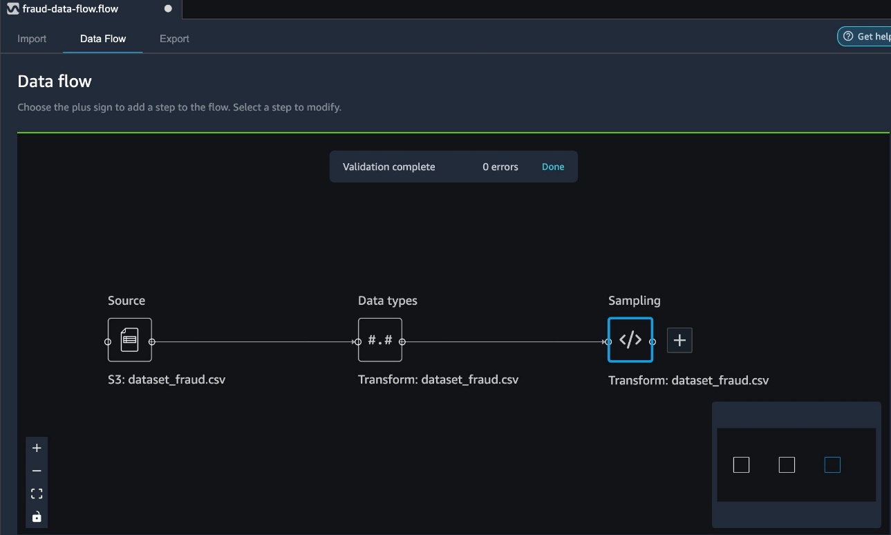
You can visualize two distinct steps on the data flow page in Data Wrangler. The first step indicates the loading of the sample dataset based on the sampling strategy you defined. After the data is loaded, Data Wrangler performs auto detection of the data types for each of the columns in the dataset. This step is added by default for all datasets.
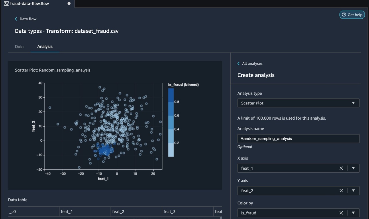
You can now review the random sampled data in Data Wrangler by adding an analysis.
- Choose the plus sign next to Data types and choose Analysis.

- For Analysis type¸ choose Scatter Plot.
- Choose feat_1 and feat_2 as for X axis and Y axis, respectively.
- For Color by, choose is_fraud.
When you’re comfortable with the dataset, proceed to do further data transformations as per your business requirement to prepare your data for ML.
In the following screenshot, we can observe the fraudulent (dark blue) and non-fraudulent (light blue) transactions in our analysis.
In the next section, we discuss using stratified sampling to ensure the fraudulent cases are chosen proportionally.
Stratified sampling with a transform
Data Wrangler allows you to sample on import, as well as sampling via a transform. In this section, we discuss using stratified sampling via a transform after you have imported your dataset into Data Wrangler.
- To initiate sampling, on the Data Flow tab, choose the plus sign next to the imported dataset and choose Add Transform.

At the time of this writing, Data Wrangler provides more than 300 built-in transformations. In addition to the built-in transforms, you can write your own custom transforms in Pandas or PySpark.
- From the Add transform list, choose Sampling.

You can now use three distinct sampling strategies: limit, random, and stratified.
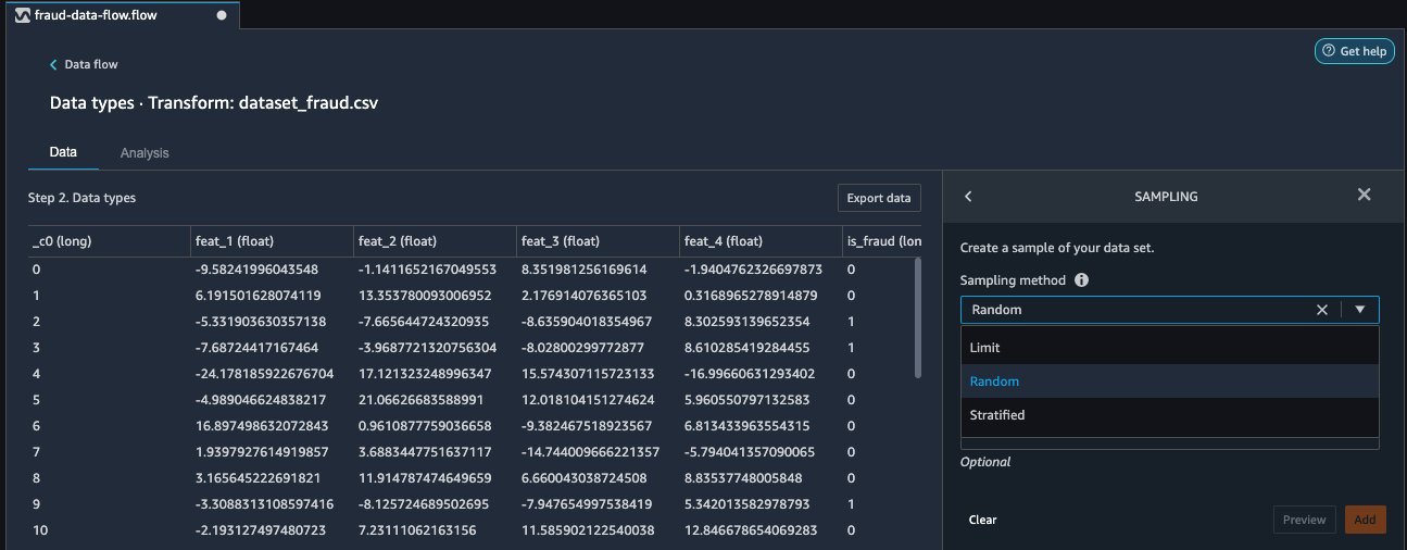
- For Sampling method, choose Stratified.
- Use the
is_fraudcolumn as the stratify column. - Choose Preview to preview the transformation, then choose Add to add this transformation as a step to your transformation recipe.

Your data flow now reflects the added sampling step.
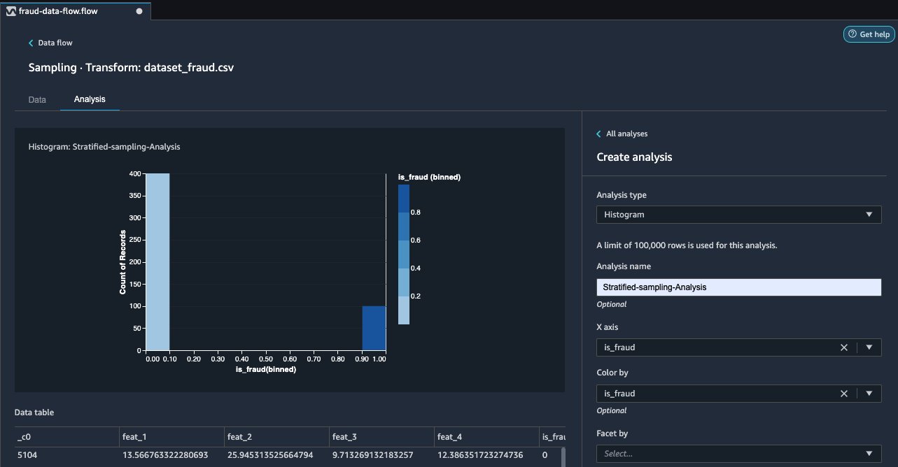
Now we can review the random sampled data by adding an analysis.
- Choose the plus sign and choose Analysis.
- For Analysis type¸ choose Histogram.
- Choose is_fraud for both X axis and Color by.
- Choose Preview.
In the following screenshot, we can observe the breakdown of fraudulent (dark blue) and non-fraudulent (light blue) cases chosen via stratified sampling in the correct proportions of 20% fraudulent and 80% non-fraudulent.
Conclusion
It is essential to sample data correctly when working with extremely large datasets and to choose the right sampling strategy to meet your business requirements. The effectiveness of your sampling relies on various factors, including business outcome, data availability, and distribution. In this post, we covered how to use Data Wrangler and its built-in sampling strategies to prepare your data.
You can start using this capability today in all Regions where SageMaker Studio is available. To get started, visit Prepare ML Data with Amazon SageMaker Data Wrangler.
Acknowledgements
The authors would like to thank Jonathan Chung (Applied Scientist) for his review and valuable feedback on this article.
About the Authors
 Ben Harris is a software engineer with experience designing, deploying, and maintaining scalable data pipelines and machine learning solutions across a variety of domains.
 Vishaal Kapoor is a Senior Applied Scientist with AWS AI. He is passionate about helping customers understand their data in Data Wrangler. In his spare time, he mountain bikes, snowboards, and spends time with his family.
 Meenakshisundaram Thandavarayan is a Senior AI/ML specialist with AWS. He helps Hi-Tech strategic accounts on their AI and ML journey. He is very passionate about data-driven AI.
 Ajai Sharma is a Principal Product Manager for Amazon SageMaker where he focuses on Data Wrangler, a visual data preparation tool for data scientists. Prior to AWS, Ajai was a Data Science Expert at McKinsey and Company, where he led ML-focused engagements for leading finance and insurance firms worldwide. Ajai is passionate about data science and loves to explore the latest algorithms and machine learning techniques.