Reducing false positives for rare events, adapting Echo hardware to ultrasound sensing, and enabling concurrent ultrasound sensing and music playback are just a few challenges Amazon researchers addressed.Read More
Artificial intelligence system learns concepts shared across video, audio, and text
Humans observe the world through a combination of different modalities, like vision, hearing, and our understanding of language. Machines, on the other hand, interpret the world through data that algorithms can process.
So, when a machine “sees” a photo, it must encode that photo into data it can use to perform a task like image classification. This process becomes more complicated when inputs come in multiple formats, like videos, audio clips, and images.
“The main challenge here is, how can a machine align those different modalities? As humans, this is easy for us. We see a car and then hear the sound of a car driving by, and we know these are the same thing. But for machine learning, it is not that straightforward,” says Alexander Liu, a graduate student in the Computer Science and Artificial Intelligence Laboratory (CSAIL) and first author of a paper tackling this problem.
Liu and his collaborators developed an artificial intelligence technique that learns to represent data in a way that captures concepts which are shared between visual and audio modalities. For instance, their method can learn that the action of a baby crying in a video is related to the spoken word “crying” in an audio clip.
Using this knowledge, their machine-learning model can identify where a certain action is taking place in a video and label it.
It performs better than other machine-learning methods at cross-modal retrieval tasks, which involve finding a piece of data, like a video, that matches a user’s query given in another form, like spoken language. Their model also makes it easier for users to see why the machine thinks the video it retrieved matches their query.
This technique could someday be utilized to help robots learn about concepts in the world through perception, more like the way humans do.
Joining Liu on the paper are CSAIL postdoc SouYoung Jin; grad students Cheng-I Jeff Lai and Andrew Rouditchenko; Aude Oliva, senior research scientist in CSAIL and MIT director of the MIT-IBM Watson AI Lab; and senior author James Glass, senior research scientist and head of the Spoken Language Systems Group in CSAIL. The research will be presented at the Annual Meeting of the Association for Computational Linguistics.
Learning representations
The researchers focus their work on representation learning, which is a form of machine learning that seeks to transform input data to make it easier to perform a task like classification or prediction.
The representation learning model takes raw data, such as videos and their corresponding text captions, and encodes them by extracting features, or observations about objects and actions in the video. Then it maps those data points in a grid, known as an embedding space. The model clusters similar data together as single points in the grid. Each of these data points, or vectors, is represented by an individual word.
For instance, a video clip of a person juggling might be mapped to a vector labeled “juggling.”
The researchers constrain the model so it can only use 1,000 words to label vectors. The model can decide which actions or concepts it wants to encode into a single vector, but it can only use 1,000 vectors. The model chooses the words it thinks best represent the data.
Rather than encoding data from different modalities onto separate grids, their method employs a shared embedding space where two modalities can be encoded together. This enables the model to learn the relationship between representations from two modalities, like video that shows a person juggling and an audio recording of someone saying “juggling.”
To help the system process data from multiple modalities, they designed an algorithm that guides the machine to encode similar concepts into the same vector.
“If there is a video about pigs, the model might assign the word ‘pig’ to one of the 1,000 vectors. Then if the model hears someone saying the word ‘pig’ in an audio clip, it should still use the same vector to encode that,” Liu explains.
A better retriever
They tested the model on cross-modal retrieval tasks using three datasets: a video-text dataset with video clips and text captions, a video-audio dataset with video clips and spoken audio captions, and an image-audio dataset with images and spoken audio captions.
For example, in the video-audio dataset, the model chose 1,000 words to represent the actions in the videos. Then, when the researchers fed it audio queries, the model tried to find the clip that best matched those spoken words.
“Just like a Google search, you type in some text and the machine tries to tell you the most relevant things you are searching for. Only we do this in the vector space,” Liu says.
Not only was their technique more likely to find better matches than the models they compared it to, it is also easier to understand.
Because the model could only use 1,000 total words to label vectors, a user can more see easily which words the machine used to conclude that the video and spoken words are similar. This could make the model easier to apply in real-world situations where it is vital that users understand how it makes decisions, Liu says.
The model still has some limitations they hope to address in future work. For one, their research focused on data from two modalities at a time, but in the real world humans encounter many data modalities simultaneously, Liu says.
“And we know 1,000 words works on this kind of dataset, but we don’t know if it can be generalized to a real-world problem,” he adds.
Plus, the images and videos in their datasets contained simple objects or straightforward actions; real-world data are much messier. They also want to determine how well their method scales up when there is a wider diversity of inputs.
This research was supported, in part, by the MIT-IBM Watson AI Lab and its member companies, Nexplore and Woodside, and by the MIT Lincoln Laboratory.
Alpa: Automated Model-Parallel Deep Learning
Over the last several years, the rapidly growing size of deep learning models has quickly exceeded the memory capacity of single accelerators. Earlier models like BERT (with a parameter size of < 1GB) can efficiently scale across accelerators by leveraging data parallelism in which model weights are duplicated across accelerators while only partitioning and distributing the training data. However, recent large models like GPT-3 (with a parameter size of 175GB) can only scale using model parallel training, where a single model is partitioned across different devices.
While model parallelism strategies make it possible to train large models, they are more complex in that they need to be specifically designed for target neural networks and compute clusters. For example, Megatron-LM uses a model parallelism strategy to split the weight matrices by rows or columns and then synchronizes results among devices. Device placement or pipeline parallelism partitions different operators in a neural network into multiple groups and the input data into micro-batches that are executed in a pipelined fashion. Model parallelism often requires significant effort from system experts to identify an optimal parallelism plan for a specific model. But doing so is too onerous for most machine learning (ML) researchers whose primary focus is to run a model and for whom the model’s performance becomes a secondary priority. As such, there remains an opportunity to automate model parallelism so that it can easily be applied to large models.
In “Alpa: Automating Inter- and Intra-Operator Parallelism for Distributed Deep Learning”, published at OSDI 2022, we describe a method for automating the complex model parallelism process. We demonstrate that with only one line of code Alpa can transform any JAX neural network into a distributed version with an optimal parallelization strategy that can be executed on a user-provided device cluster. We are also excited to release Alpa’s code to the broader research community.
Alpa Design
We begin by grouping existing ML parallelization strategies into two categories, inter-operator parallelism and intra-operator parallelism. Inter-operator parallelism assigns distinct operators to different devices (e.g., device placement) that are often accelerated with a pipeline execution schedule (e.g., pipeline parallelism). With intra-operator parallelism, which includes data parallelism (e.g., Deepspeed-Zero), operator parallelism (e.g., Megatron-LM), and expert parallelism (e.g., GShard-MoE), individual operators are split and executed on multiple devices, and often collective communication is used to synchronize the results across devices.
The difference between these two approaches maps naturally to the heterogeneity of a typical compute cluster. Inter-operator parallelism has lower communication bandwidth requirements because it is only transmitting activations between operators on different accelerators. But, it suffers from device underutilization because of its pipeline data dependency, i.e., some operators are inactive while waiting on the outputs from other operators. In contrast, intra-operator parallelism doesn’t have the data dependency issue, but requires heavier communication across devices. In a GPU cluster, the GPUs within a node have higher communication bandwidth that can accommodate intra-operator parallelism. However, GPUs across different nodes are often connected with much lower bandwidth (e.g., ethernet) so inter-operator parallelism is preferred.
By leveraging heterogeneous mapping, we design Alpa as a compiler that conducts various passes when given a computational graph and a device cluster from a user. First, the inter-operator pass slices the computational graph into subgraphs and the device cluster into submeshes (i.e., a partitioned device cluster) and identifies the best way to assign a subgraph to a submesh. Then, the intra-operator pass finds the best intra-operator parallelism plan for each pipeline stage from the inter-operator pass. Finally, the runtime orchestration pass generates a static plan that orders the computation and communication and executes the distributed computational graph on the actual device cluster.
 |
| An overview of Alpa. In the sliced subgraphs, red and blue represent the way the operators are partitioned and gray represents operators that are replicated. Green represents the actual devices (e.g., GPUs). |
Intra-Operator Pass
Similar to previous research (e.g., Mesh-TensorFlow and GSPMD), intra-operator parallelism partitions a tensor on a device mesh. This is shown below for a typical 3D tensor in a Transformer model with a given batch, sequence, and hidden dimensions. The batch dimension is partitioned along device mesh dimension 0 (mesh0), the hidden dimension is partitioned along mesh dimension 1 (mesh1), and the sequence dimension is replicated to each processor.
 |
| A 3D tensor that is partitioned on a 2D device mesh. |
With the partitions of tensors in Alpa, we further define a set of parallelization strategies for each individual operator in a computational graph. We show example parallelization strategies for matrix multiplication in the figure below. Defining parallelization strategies on operators leads to possible conflicts on the partitions of tensors because one tensor can be both the output of one operator and the input of another. In this case, re-partition is needed between the two operators, which incurs additional communication costs.
 |
| The parallelization strategies for matrix multiplication. |
Given the partitions of each operator and re-partition costs, we formulate the intra-operator pass as a Integer-Linear Programming (ILP) problem. For each operator, we define a one-hot variable vector to enumerate the partition strategies. The ILP objective is to minimize the sum of compute and communication cost (node cost) and re-partition communication cost (edge cost). The solution of the ILP translates to one specific way to partition the original computational graph.
 |
Inter-Operator Pass
The inter-operator pass slices the computational graph and device cluster for pipeline parallelism. As shown below, the boxes represent micro-batches of input and the pipeline stages represent a submesh executing a subgraph. The horizontal dimension represents time and shows the pipeline stage at which a micro-batch is executed. The goal of the inter-operator pass is to minimize the total execution latency, which is the sum of the entire workload execution on the device as illustrated in the figure below. Alpa uses a Dynamic Programming (DP) algorithm to minimize the total latency. The computational graph is first flattened, and then fed to the intra-operator pass where the performance of all possible partitions of the device cluster into submeshes are profiled.
 |
| Pipeline parallelism. For a given time, this figure shows the micro-batches (colored boxes) that a partitioned device cluster and a sliced computational graph (e.g., stage 1, 2, 3) is processing. |
Runtime Orchestration
After the inter- and intra-operator parallelization strategies are complete, the runtime generates and dispatches a static sequence of execution instructions for each device submesh. These instructions include RUN a specific subgraph, SEND/RECEIVE tensors from other meshes, or DELETE a specific tensor to free the memory. The devices can execute the computational graph without other coordination by following the instructions.
Evaluation
We test Alpa with eight AWS p3.16xlarge instances, each of which has eight 16 GB V100 GPUs, for 64 total GPUs. We examine weak scaling results of growing the model size while increasing the number of GPUs. We evaluate three models: (1) the standard Transformer model (GPT); (2) the GShard-MoE model, a transformer with mixture-of-expert layers; and (3) Wide-ResNet, a significantly different model with no existing expert-designed model parallelization strategy. The performance is measured by peta-floating point operations per second (PFLOPS) achieved on the cluster.
We demonstrate that for GPT, Alpa outputs a parallelization strategy very similar to the one computed by the best existing framework, Megatron-ML, and matches its performance. For GShard-MoE, Alpa outperforms the best expert-designed baseline on GPU (i.e., Deepspeed) by up to 8x. Results for Wide-ResNet show that Alpa can generate the optimal parallelization strategy for models that have not been studied by experts. We also show the linear scaling numbers for reference.

|
| GPT: Alpa matches the performance of Megatron-ML, the best expert-designed framework. |
 |
| GShard MoE: Alpa outperforms Deepspeed (the best expert-designed framework on GPU) by up to 8x. |
 |
| Wide-ResNet: Alpa generalizes to models without manual plans. Pipeline and Data Parallelism (PP-DP) is a baseline model that uses only pipeline and data parallelism but no other intra-operator parallelism. |
 |
| The parallelization strategy for Wide-ResNet on 16 GPUs consists of three pipeline stages and is a complicated strategy even for an expert to design. Stages 1 and 2 are on 4 GPUs performing data parallelism, and stage 3 is on 8 GPUs performing operator parallelism. |
Conclusion
The process of designing an effective parallelization plan for distributed model-parallel deep learning has historically been a difficult and labor-intensive task. Alpa is a new framework that leverages intra- and inter-operator parallelism for automated model-parallel distributed training. We believe that Alpa will democratize distributed model-parallel learning and accelerate the development of large deep learning models. Explore the open-source code and learn more about Alpa in our paper.
Acknowledgements
Thanks to the co-authors of the paper: Lianmin Zheng, Hao Zhang, Yonghao Zhuang, Yida Wang, Danyang Zhuo, Joseph E. Gonzalez, and Ion Stoica. We would also like to thank Shibo Wang, Jinliang Wei, Yanping Huang, Yuanzhong Xu, Zhifeng Chen, Claire Cui, Naveen Kumar, Yash Katariya, Laurent El Shafey, Qiao Zhang, Yonghui Wu, Marcello Maggioni, Mingyao Yang, Michael Isard, Skye Wanderman-Milne, and David Majnemer for their collaborations to this research.

Ankan Bansal’s long journey into the world of computer vision
How a math-loving student travelled 7,000 miles to pursue a passion and wound up becoming an applied scientist.Read More
Rethinking Human-in-the-Loop for Artificial Augmented Intelligence
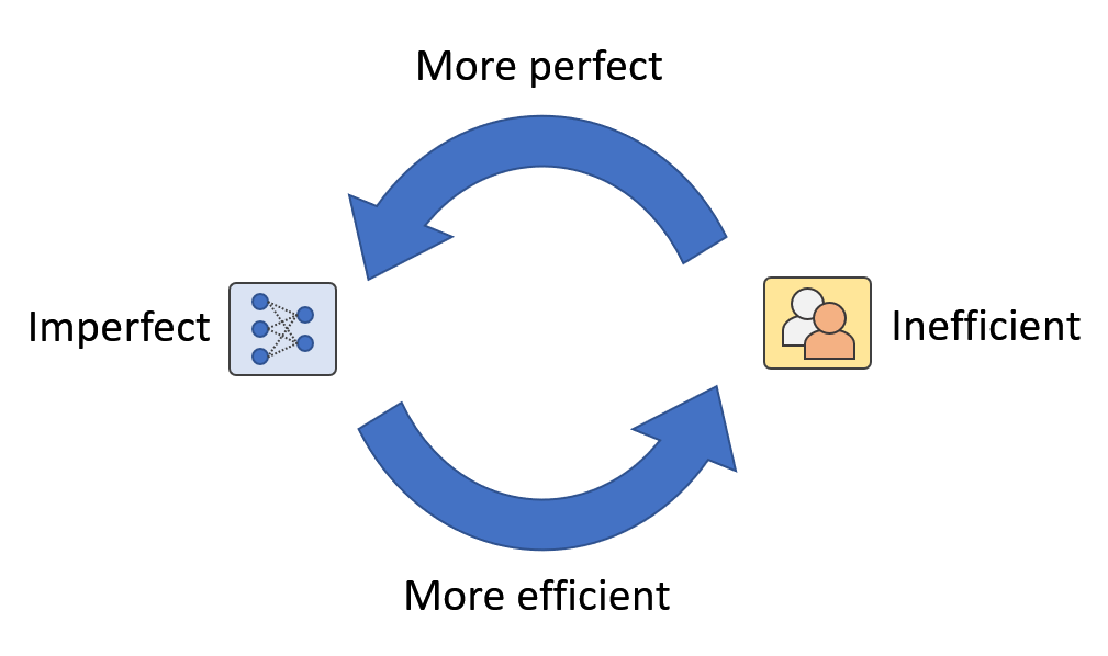
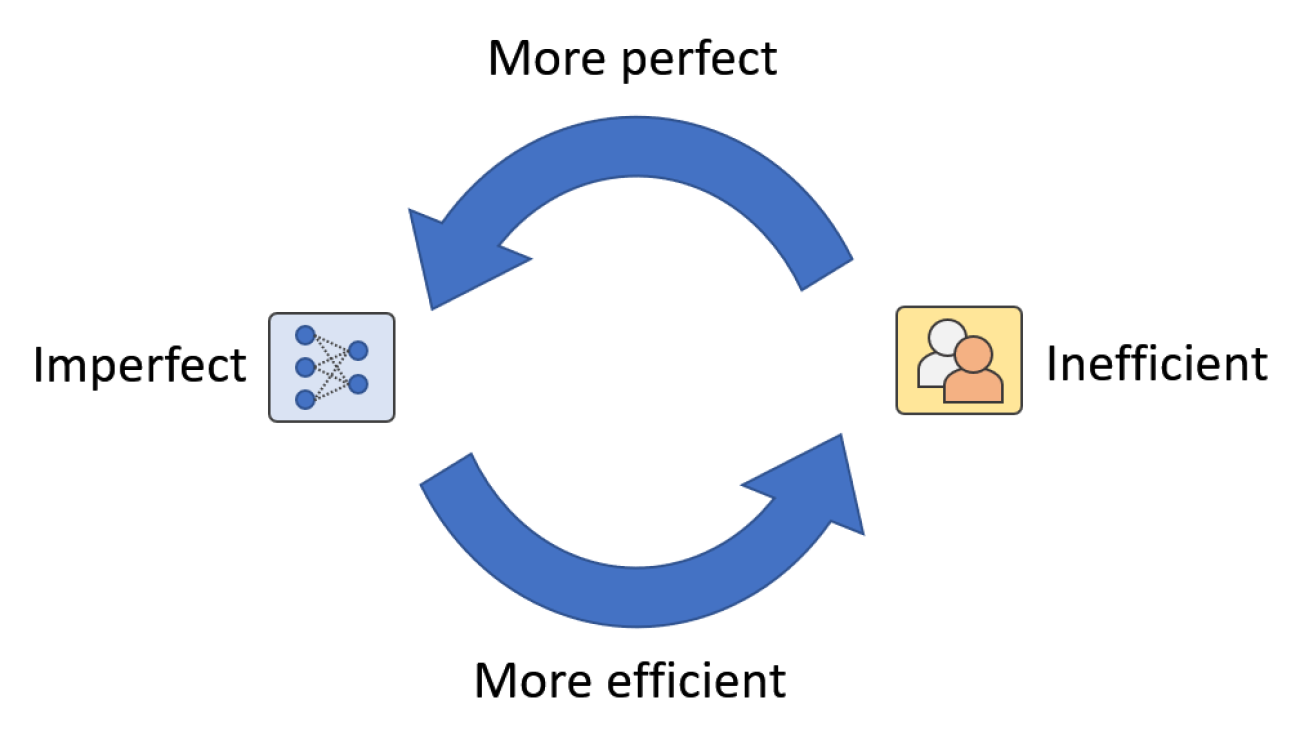
Figure 1: In real-world applications, we think there exist a human-machine loop where humans and machines are mutually augmenting each other. We call it Artificial Augmented Intelligence.
How do we build and evaluate an AI system for real-world applications? In most AI research, the evaluation of AI methods involves a training-validation-testing process. The experiments usually stop when the models have good testing performance on the reported datasets because real-world data distribution is assumed to be modeled by the validation and testing data. However, real-world applications are usually more complicated than a single training-validation-testing process. The biggest difference is the ever-changing data. For example, wildlife datasets change in class composition all the time because of animal invasion, re-introduction, re-colonization, and seasonal animal movements. A model trained, validated, and tested on existing datasets can easily be broken when newly collected data contain novel species. Fortunately, we have out-of-distribution detection methods that can help us detect samples of novel species. However, when we want to expand the recognition capacity (i.e., being able to recognize novel species in the future), the best we can do is fine-tuning the models with new ground-truthed annotations. In other words, we need to incorporate human effort/annotations regardless of how the models perform on previous testing sets.
Rethinking Human-in-the-Loop for Artificial Augmented Intelligence
Figure 1: In real-world applications, we think there exist a human-machine loop where humans and machines are mutually augmenting each other. We call it Artificial Augmented Intelligence.
How do we build and evaluate an AI system for real-world applications? In most AI research, the evaluation of AI methods involves a training-validation-testing process. The experiments usually stop when the models have good testing performance on the reported datasets because real-world data distribution is assumed to be modeled by the validation and testing data. However, real-world applications are usually more complicated than a single training-validation-testing process. The biggest difference is the ever-changing data. For example, wildlife datasets change in class composition all the time because of animal invasion, re-introduction, re-colonization, and seasonal animal movements. A model trained, validated, and tested on existing datasets can easily be broken when newly collected data contain novel species. Fortunately, we have out-of-distribution detection methods that can help us detect samples of novel species. However, when we want to expand the recognition capacity (i.e., being able to recognize novel species in the future), the best we can do is fine-tuning the models with new ground-truthed annotations. In other words, we need to incorporate human effort/annotations regardless of how the models perform on previous testing sets.
‘In the NVIDIA Studio’ Welcomes Concept Designer Yangtian Li
Editor’s note: This post is part of our weekly In the NVIDIA Studio series, which celebrates featured artists, offers creative tips and tricks, and demonstrates how NVIDIA Studio technology accelerates creative workflows.
This week In the NVIDIA Studio, we welcome Yangtian Li, a senior concept artist at Singularity6.
Li is a concept designer and illustrator who has worked on some of the biggest video game franchises, including Call of Duty, Magic: the Gathering and Vainglory. Her artwork also appears in book illustrations and magazines.

Li’s impressive portfolio features character portraits of strong, graceful, empowered women. Their backstories and elegance are inspired by her own life experiences and world travels.

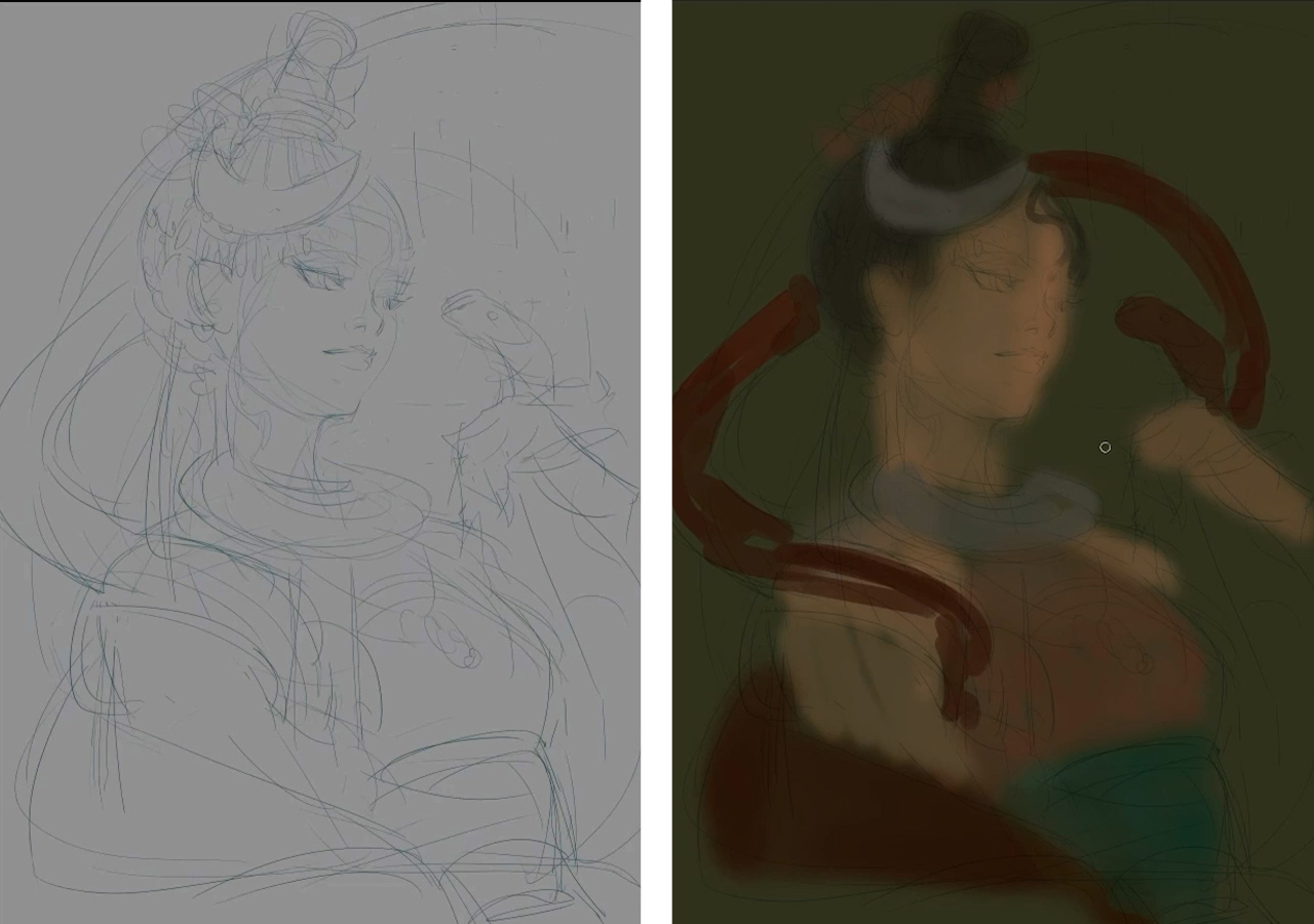
Now based in Seattle, Li’s artistic journey began in Chengdu, China. Her hometown serves as the inspiration behind her extraordinary portrait, Snake Witch. This unique and provoking work is based on tribal black magic from Chinese folklore. Li drew and painted the piece, powered by a GeForce RTX GPU and the NVIDIA Studio platform.

Snake Witch is a product of Li’s fascination with black magic, or “Gu,” where tribal witch doctors would gather toxic creatures, use their venom to make poison and practice the dark arts. “I always thought the stories were fascinating, so I wanted to do a take,” Li said. “Snakes are more appealing to me, and it helps to create some interesting compositions.”
After primarily working in 2D, Li moves to 3D to support her concept process. She adds, “having a high-end GPU really helps speed up the process when it comes to using Blender, Zbrush and so on.” These speed-ups, she says, are particularly noticeable with GPU-accelerated rendering in Blender Cycles 3.0, achieving results that are over 5x faster with a GeForce RTX laptop GPU compared to a MacBook Pro M1 Max or CPU alone.
With the Snake Witch’s character foundation in a good place, Li used the Liquify filter to subtly distort her subject’s facial features.
Liquify is one of over 30 GPU-accelerated features in Adobe Photoshop, like AI-powered Neural Filters, that help artists explore creative ideas and make complex adjustments in seconds.
“The more life experiences you have, your understanding of the world evolves, and that will be reflected in your art.”
Li uses adjustment layers in the coloring phase of her process, allowing for non-destructive edits while trying to achieve the correct color tone.
If unsatisfied with an adjustment, Li can simply delete it while the original image remains intact.
Finally, Li adjusts lighting, using the Opacity feature to block light from right of the image, adding a modicum of realistic flair.

Remaining in a productive flow state is critical for Li, as it is for many artists, and her GeForce RTX GPU allows her to spend more time in that magical creative zone where ideas come to life faster and more naturally.
Li goes into greater detail on how she created Snake Witch in her Studio Session. This three-part series includes her processes for initial sketching, color and detail optimization, and finishing touches.

Check out Li’s portfolio and favorite projects on Instagram.
Accelerating Adobe Creators In the NVIDIA Studio
More resources are available to creators seeking additional NVIDIA Studio features and optimizations that accelerate Adobe creative apps.
Follow a step-by-step tutorial in Photoshop that details how to apply a texture from a photo to a 3D visualization render.
Learn how to work significantly faster in Adobe Lightroom by utilizing AI-powered masking tools; Select Subject and Select Sky.
Follow NVIDIA Studio on Facebook, Twitter and Instagram, access tutorials on the Studio YouTube channel, and get updates directly in your inbox by joining the NVIDIA Studio newsletter.
The post ‘In the NVIDIA Studio’ Welcomes Concept Designer Yangtian Li appeared first on NVIDIA Blog.
Data Incubation – Synthesizing Missing Data for Handwriting Recognition
In this paper, we demonstrate how a generative model can be used to build a better recognizer through the control of content and style. We are building an online handwriting recognizer from a modest amount of training samples. By training our controllable handwriting synthesizer on the same data, we can synthesize handwriting with previously underrepresented content (e.g., URLs and email addresses) and style (e.g., cursive and slanted). Moreover, we propose a framework to analyze a recognizer that is trained with a mixture of real and synthetic training data. We use the framework to optimize…Apple Machine Learning Research
Achieve hyperscale performance for model serving using NVIDIA Triton Inference Server on Amazon SageMaker
Machine learning (ML) applications are complex to deploy and often require multiple ML models to serve a single inference request. A typical request may flow across multiple models with steps like preprocessing, data transformations, model selection logic, model aggregation, and postprocessing. This has led to the evolution of common design patterns such as serial inference pipelines, ensembles (scatter gather), and business logic workflows, resulting in realizing the entire workflow of the request as a Directed Acyclic Graph (DAG). However, as workflows get more complex, this leads to an increase in overall response times, or latency, of these applications which in turn impacts the overall user experience. Furthermore, if these components are hosted on different instances, the additional network latency between these instances increases the overall latency. Consider an example of a popular ML use case for a virtual assistant in customer support. A typical request might have to go through several steps involving speech recognition, natural language processing (NLP), dialog state tracking, dialog policy, text generation, and finally text to speech. Furthermore, to make the user interaction more personalized, you might also use state-of-art, transformer-based NLP models like different versions of BERT, BART, and GPT. The end result is long response times for these model ensembles and a poor customer experience.
A common pattern to drive lower response times without compromising overall throughput is to host these models on the same instance along with the lightweight business logic embedded in it. These models can further be encapsulated within single or multiple containers on the same instance in order to provide isolation for running processes and keep latency low. Additionally, overall latency also depends on inference application logic, model optimizations, underlying infrastructure (including compute, storage, and networking), and the underlying web server taking inference requests. NVIDIA Triton Inference Server is an open-source inference serving software with features to maximize throughput and hardware utilization with ultra-low (single-digit milliseconds) inference latency. It has wide support of ML frameworks (including TensorFlow, PyTorch, ONNX, XGBoost, and NVIDIA TensorRT) and infrastructure backends, including GPUs, CPUs, and AWS Inferentia. Additionally, Triton Inference Server is integrated with Amazon SageMaker, a fully managed end-to-end ML service, providing real-time inference options including single and multi-model hosting. These inference options include hosting multiple models within the same container behind a single endpoint, and hosting multiple models with multiple containers behind a single endpoint.
In November 2021, we announced the integration of Triton Inference Server on SageMaker. AWS worked closely with NVIDIA to enable you to get the best of both worlds and make model deployment with Triton on AWS easier.
In this post, we look at best practices for deploying transformer models at scale on GPUs using Triton Inference Server on SageMaker. First, we start with a summary of key concepts around latency in SageMaker, and an overview of performance tuning guidelines. Next, we provide an overview of Triton and its features as well as example code for deploying on SageMaker. Finally, we perform load tests using SageMaker Inference Recommender and summarize the insights and conclusions from load testing of a popular transformer model provided by Hugging Face.
You can review the notebook we used to deploy models and perform load tests on your own using the code on GitHub.
Performance tuning and optimization for model serving on SageMaker
Performance tuning and optimization is an empirical process often involving multiple iterations. The number of parameters to tune is combinatorial and the set of configuration parameter values aren’t independent of each other. Various factors affect optimal parameter tuning, including payload size, type, and the number of ML models in the inference request flow graph, storage type, compute instance type, network infrastructure, application code, inference serving software runtime and configuration, and more.
If you’re using SageMaker for deploying ML models, you have to select a compute instance with the best price-performance, which is a complicated and iterative process that can take weeks of experimentation. First, you need to choose the right ML instance type out of over 70 options based on the resource requirements of your models and the size of the input data. Next, you need to optimize the model for the selected instance type. Lastly, you need to provision and manage infrastructure to run load tests and tune cloud configuration for optimal performance and cost. All this can delay model deployment and time to market. Additionally, you need to evaluate the trade-offs between latency, throughput, and cost to select the optimal deployment configuration. SageMaker Inference Recommender automatically selects the right compute instance type, instance count, container parameters, and model optimizations for inference to maximize throughput, reduce latency, and minimize cost.
Real-time inference and latency in SageMaker
SageMaker real-time inference is ideal for inference workloads where you have real-time, interactive, low-latency requirements. There are four most commonly used metrics for monitoring inference request latency for SageMaker inference endpoints
- Container latency – The time it takes to send the request, fetch the response from the model’s container, and complete inference in the container. This metric is available in Amazon CloudWatch as part of the Invocation Metrics published by SageMaker.
- Model latency – The total time taken by all SageMaker containers in an inference pipeline. This metric is available in Amazon CloudWatch as part of the Invocation Metrics published by SageMaker.
- Overhead latency – Measured from the time that SageMaker receives the request until it returns a response to the client, minus the model latency. This metric is available in Amazon CloudWatch as part of the Invocation Metrics published by SageMaker.
- End-to-end latency – Measured from the time the client sends the inference request until it receives a response back. Customers can publish this as a custom metric in Amazon CloudWatch.
The following diagram illustrates these components.

Container latency depends on several factors; the following are among the most important:
- Underlying protocol (HTTP(s)/gRPC) used to communicate with the inference server
- Overhead related to creating new TLS connections
- Deserialization time of the request/response payload
- Request queuing and batching features provided by the underlying inference server
- Request scheduling capabilities provided by the underlying inference server
- Underlying runtime performance of the inference server
- Performance of preprocessing and postprocessing libraries before calling the model prediction function
- Underlying ML framework backend performance
- Model-specific and hardware-specific optimizations
In this post, we focus primarily on optimizing container latency along with overall throughput and cost. Specifically, we explore performance tuning Triton Inference Server running inside a SageMaker container.
Use case overview
Deploying and scaling NLP models in a production setup can be quite challenging. NLP models are often very large in size, containing millions of model parameters. Optimal model configurations are required to satisfy the stringent performance and scalability requirements of production-grade NLP applications.
In this post, we benchmark an NLP use case using a SageMaker real-time endpoint based on a Triton Inference Server container and recommend performance tuning optimizations for our ML use case. We use a large, pre-trained transformer-based Hugging Face BERT large uncased model, which has about 336 million model parameters. The input sentence used for the binary classification model is padded and truncated to a maximum input sequence length of 512 tokens. The inference load test simulates 500 invocations per second (30,000 maximum invocations per minute) and ModelLatency of less than 0.5 seconds (500 milliseconds).
The following table summarizes our benchmark configuration.
| Model Name | Hugging Face bert-large-uncased
|
| Model Size | 1.25 GB |
| Latency Requirement | 0.5 seconds (500 milliseconds) |
| Invocations per Second | 500 requests (30,000 per minute) |
| Input Sequence Length | 512 tokens |
| ML Task | Binary classification |
NVIDIA Triton Inference Server
Triton Inference Server is specifically designed to enable scalable, rapid, and easy deployment of models in production. Triton supports a variety of major AI frameworks, including TensorFlow, TensorRT, PyTorch, XGBoost and ONNX. With the Python and C++ custom backend, you can also implement your inference workload for more customized use cases.
Most importantly, Triton provides a simple configuration-based setup to host your models, which exposes a rich set of performance optimization features you can use with little coding effort.
Triton increases inference performance by maximizing hardware utilization with different optimization techniques (concurrent model runs and dynamic batching are the most frequently used). Finding the optimal model configurations from various combinations of dynamic batch sizes and the number of concurrent model instances is key to achieving real time inference within low-cost serving using Triton.
Dynamic batching
Many practitioners tend to run inference sequentially when the server is invoked with multiple independent requests. Although easier to set up, it’s usually not the best practice to utilize GPU’s compute power. To address this, Triton offers the built-in optimizations of dynamic batching to combine these independent inference requests on the server side to form a larger batch dynamically to increase throughput. The following diagram illustrates the Triton runtime architecture.
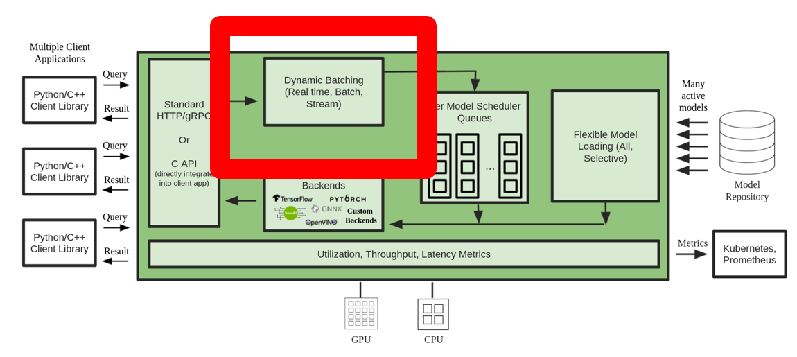
In the preceding architecture, all the requests reach the dynamic batcher first before entering the actual model scheduler queues to wait for inference. You can set your preferred batch sizes for dynamic batching using the preferred_batch_size settings in the model configuration. (Note that the formed batch size needs to be less than the max_batch_size the model supports.) You can also configure max_queue_delay_microseconds to specify the maximum delay time in the batcher to wait for other requests to join the batch based on your latency requirements.
The following code snippet shows how you can add this feature with model configuration files to set dynamic batching with a preferred batch size of 16 for the actual inference. With the current settings, the model instance is invoked instantly when the preferred batch size of 16 is met or the delay time of 100 microseconds has elapsed since the first request reached the dynamic batcher.
Running models concurrently
Another essential optimization offered in Triton to maximize hardware utilization without additional latency overhead is concurrent model execution, which allows multiple models or multiple copies of the same model to run in parallel. This feature enables Triton to handle multiple inference requests simultaneously, which increases the inference throughput by utilizing otherwise idle compute power on the hardware.
The following figure showcases how you can easily configure different model deployment policies with only a few lines of code changes. For example, configuration A (left) shows that you can broadcast the same configuration of two model instances of bert-large-uncased to all available GPUs. In contrast, configuration B (middle) shows a different configuration for GPU 0 only, without changing the policies on the other GPUs. You can also deploy instances of different models on a single GPU, as shown in configuration C (right).
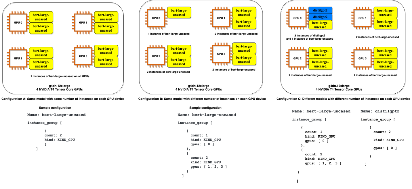
In configuration C, the compute instance can handle two concurrent requests for the DistilGPT-2 model and seven concurrent requests for the bert-large-uncased model in parallel. With these optimizations, the hardware resources can be better utilized for the serving process, thereby improving the throughput and providing better cost-efficiency for your workload.
TensorRT
NVIDIA TensorRT is an SDK for high-performance deep learning inference that works seamlessly with Triton. TensorRT, which supports every major deep learning framework, includes an inference optimizer and runtime that delivers low latency and high throughput to run inferences with massive volumes of data via powerful optimizations.
TensorRT optimizes the graph to minimize memory footprint by freeing unnecessary memory and efficiently reusing it. Additionally, TensorRT compilation fuses the sparse operations inside the model graph to form a larger kernel to avoid the overhead of multiple small kernel launches. Kernel auto-tuning helps you fully utilize the hardware by selecting the best algorithm on your target GPU. CUDA streams enable models to run in parallel to maximize your GPU utilization for best performance. Last but not least, the quantization technique can fully use the mixed-precision acceleration of the Tensor cores to run the model in FP32, TF32, FP16, and INT8 to achieve the best inference performance.
Triton on SageMaker hosting
SageMaker hosting services are the set of SageMaker features aimed at making model deployment and serving easier. It provides a variety of options to easily deploy, auto scale, monitor, and optimize ML models tailored for different use cases. This means that you can optimize your deployments for all types of usage patterns, from persistent and always available with serverless options, to transient, long-running, or batch inference needs.
Under the SageMaker hosting umbrella is also the set of SageMaker inference Deep Learning Containers (DLCs), which come prepackaged with the appropriate model server software for their corresponding supported ML framework. This enables you to achieve high inference performance with no model server setup, which is often the most complex technical aspect of model deployment and in general, isn’t part of a data scientist’s skill set. Triton inference server is now available on SageMaker Deep Learning Containers (DLC).
This breadth of options, modularity, and ease of use of different serving frameworks makes SageMaker and Triton a powerful match.
SageMaker Inference Recommender for benchmarking test results
We use SageMaker Inference Recommender to run our experiments. SageMaker Inference Recommender offers two types of jobs: default and advanced, as illustrated in the following diagram.
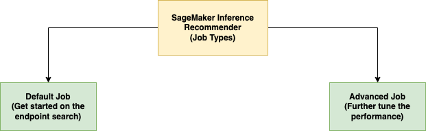
The default job provides recommendations on instance types with just the model and a sample payload to benchmark. In addition to instance recommendations, the service also offers runtime parameters that improve performance. The default job’s recommendations are intended to narrow down the instance search. In some cases, it could be the instance family, and in others, it could be the specific instance types. The results of the default job are then fed into the advanced job.
The advanced job offers more controls to further fine-tune performance. These controls simulate the real environment and production requirements. Among these controls is the traffic pattern, which aims to stage the request pattern for the benchmarks. You can set ramps or steady traffic by using the traffic pattern’s multiple phases. For example, an InitialNumberOfUsers of 1, SpawnRate of 1, and DurationInSeconds of 600 may result in ramp traffic of 10 minutes with 1 concurrent user at the beginning and 10 at the end. Additionally, on the controls, MaxInvocations and ModelLatencyThresholds set the threshold of production, so when one of the thresholds is exceeded, the benchmarking stops.
Finally, recommendation metrics include throughput, latency at maximum throughput, and cost per inference, so it’s easy to compare them.
We use the advanced job type of SageMaker Inference Recommender to run our experiments to gain additional control over the traffic patterns, and fine-tune the configuration of the serving container.
Experiment setup
We use the custom load test feature of SageMaker Inference Recommender to benchmark the NLP profile outlined in our use case. We first define the following prerequisites related to the NLP model and ML task. SageMaker Inference Recommender uses this information to pull an inference Docker image from Amazon Elastic Container Registry (Amazon ECR) and register the model with the SageMaker model registry.
| Domain | NATURAL_LANGUAGE_PROCESSING |
| Task | FILL_MASK |
| Framework | PYTORCH: 1.6.0 |
| Model | bert-large-uncased |
The traffic pattern configurations in SageMaker Inference Recommender allow us to define different phases for the custom load test. The load test starts with two initial users and spawns two new users every minute, for a total duration of 25 minutes (1500 seconds), as shown in the following code:
We experiment with load testing the same model in two different states. The PyTorch-based experiments use the standard, unaltered PyTorch model. For the TensorRT-based experiments, we convert the PyTorch model into a TensorRT engine beforehand.
We apply different combinations of the performance optimization features on these two models, summarized in the following table.
| Configuration Name | Configuration Description | Model Configuration |
pt-base |
PyTorch baseline | Base PyTorch model, no changes |
pt-db |
PyTorch with dynamic batching |
dynamic_batching{}
|
pt-ig |
PyTorch with multiple model instances |
instance_group [ { count: 2 kind: KIND_GPU } ]
|
pt-ig-db |
PyTorch with multiple model instances and dynamic batching |
dynamic_batching {},instance_group [ { count: 2 kind: KIND_GPU }]
|
trt-base |
TensorRT baseline | PyTorch model compiled with TensoRT trtexec utility |
trt-db |
TensorRT with dynamic batching |
dynamic_batching{}
|
trt-ig |
TensorRT with multiple model instances |
instance_group [ { count: 2 kind: KIND_GPU }]
|
trt-ig-db |
TensorRT with multiple model instances and dynamic batching |
dynamic_batching{},instance_group [ { count: 2 kind: KIND_GPU }]
|
Test results and observations
We conducted load tests for three instance types within the same g4dn family: ml.g4dn.xlarge, ml.g4dn.2xlarge and ml.g4dn.12xlarge. All g4dn instance types have access to NVIDIA T4 Tensor Core GPUs, and 2nd Generation Intel Cascade Lake processors. The logic behind the choice of instance types was to have both an instance with only one GPU available, as well as an instance with access to multiple GPUs—four in the case of ml.g4dn.12xlarge. Additionally, we wanted to test if increasing the vCPU capacity on the instance with only one available GPU would yield a cost-performance ratio improvement.
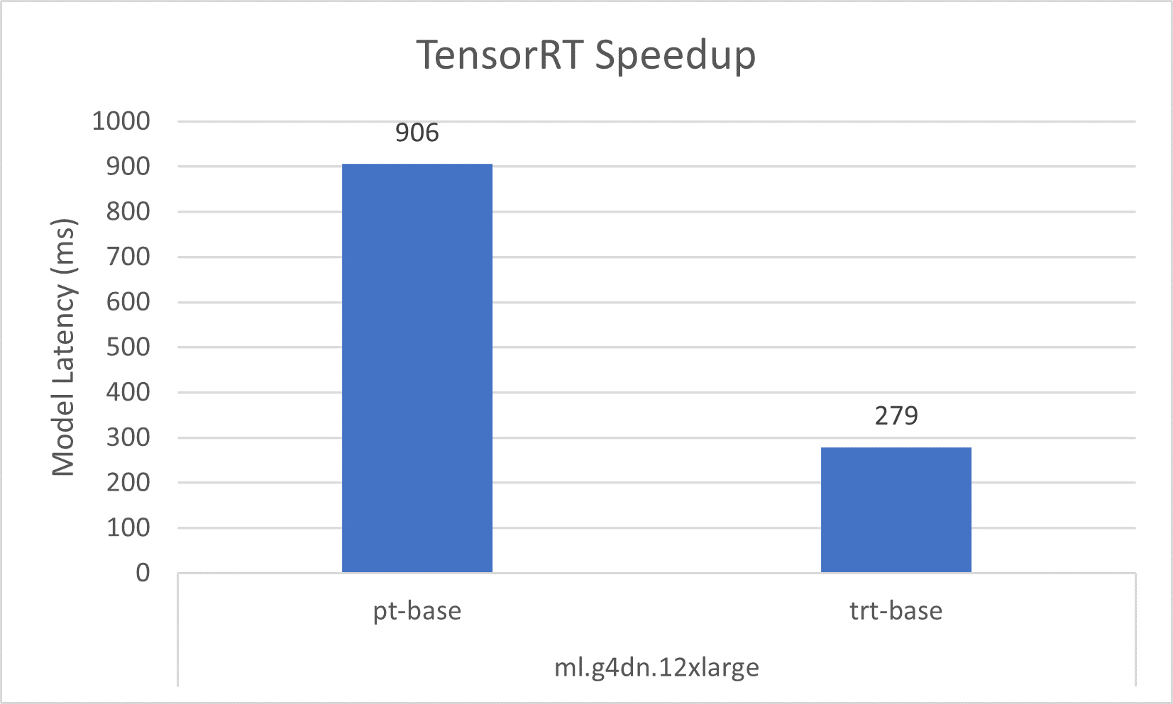
Let’s go over the speedup of the individual optimization first. The following graph shows that TensorRT optimization provides a 50% reduction in model latency compared to the native one in PyTorch on the ml.g4dn.xlarge instance. This latency reduction grows to over three times on the multi-GPU instances of ml.g4dn.12xlarge. Meanwhile, the 30% throughput improvement is consistent on both instances, resulting in better cost-effectiveness after applying TensorRT optimizations.
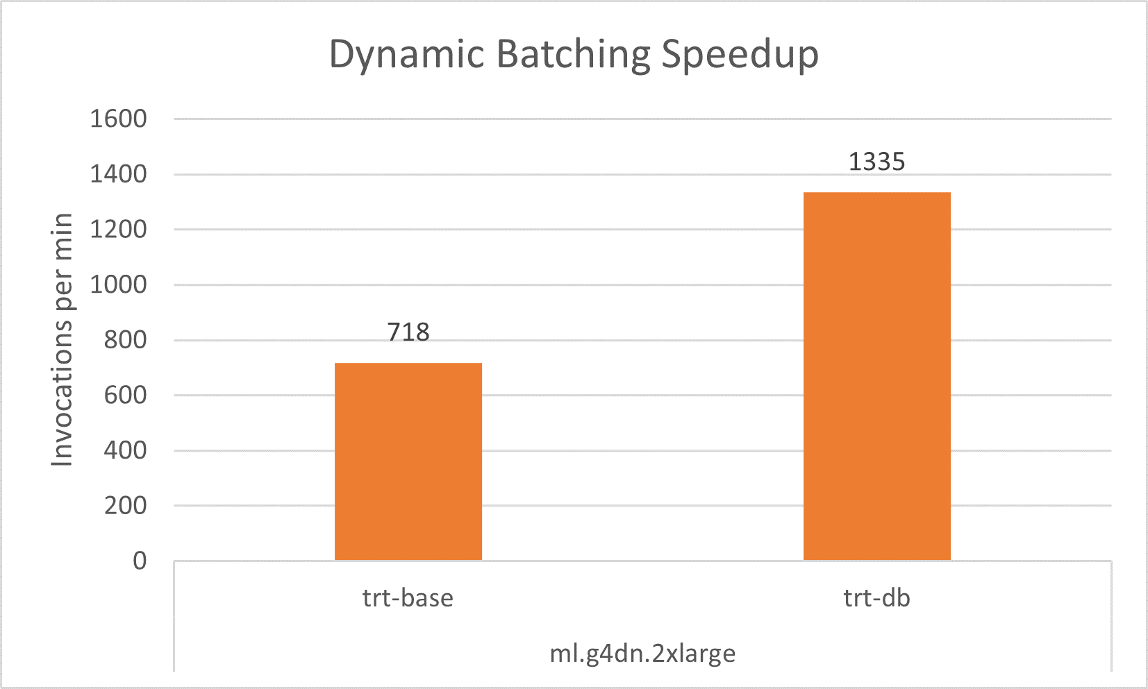
With dynamic batching, we can get close to 2x improvement in throughput using the same hardware architecture on all experiments instance of ml.g4dn.xlarge, ml.g4dn.2xlarge and ml.g4dn.12xlarge without noticeable latency increase.
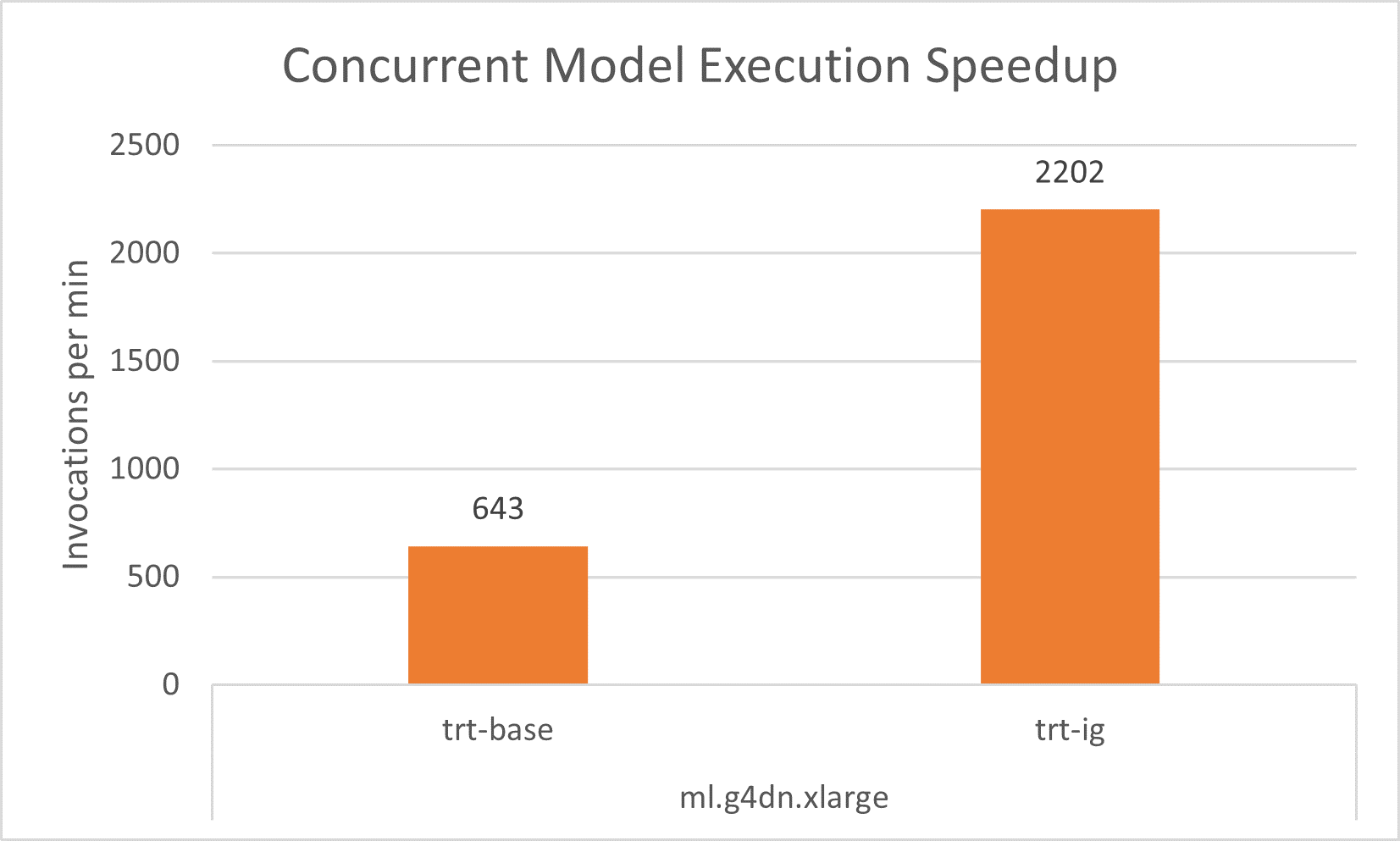
Similarly, concurrent model execution enable us to obtain about 3-4x improvement in throughput by maximizing the GPU utilization on ml.g4dn.xlarge instance and about 2x improvement on both the ml.g4dn.2xlarge instance and the multi-GPU instance of ml.g4dn.12xlarge.. This throughput increase comes without any overhead in the latency.
Better still, we can integrate all these optimizations to provide the best performance by utilizing the hardware resources to the fullest. The following table and graphs summarize the results we obtained in our experiments.
| Configuration Name | Model optimization |
Dynamic Batching |
Instance group config | Instance type | vCPUs | GPUs |
GPU Memory (GB) |
Initial Instance Count[1] | Invocations per min per Instance | Model Latency | Cost per Hour[2] |
| pt-base | NA | No | NA | ml.g4dn.xlarge | 4 | 1 | 16 | 62 | 490 | 1500 | 45.6568 |
| pt-db | NA | Yes | NA | ml.g4dn.xlarge | 4 | 1 | 16 | 57 | 529 | 1490 | 41.9748 |
| pt-ig | NA | No | 2 | ml.g4dn.xlarge | 4 | 1 | 16 | 34 | 906 | 868 | 25.0376 |
| pt-ig-db | NA | Yes | 2 | ml.g4dn.xlarge | 4 | 1 | 16 | 34 | 892 | 1158 | 25.0376 |
| trt-base | TensorRT | No | NA | ml.g4dn.xlarge | 4 | 1 | 16 | 47 | 643 | 742 | 34.6108 |
| trt-db | TensorRT | Yes | NA | ml.g4dn.xlarge | 4 | 1 | 16 | 28 | 1078 | 814 | 20.6192 |
| trt-ig | TensorRT | No | 2 | ml.g4dn.xlarge | 4 | 1 | 16 | 14 | 2202 | 1273 | 10.3096 |
| trt-db-ig | TensorRT | Yes | 2 | ml.g4dn.xlarge | 4 | 1 | 16 | 10 | 3192 | 783 | 7.364 |
| pt-base | NA | No | NA | ml.g4dn.2xlarge | 8 | 1 | 32 | 56 | 544 | 1500 | 52.64 |
| pt-db | NA | Yes | NA | ml.g4dn.2xlarge | 8 | 1 | 32 | 59 | 517 | 1500 | 55.46 |
| pt-ig | NA | No | 2 | ml.g4dn.2xlarge | 8 | 1 | 32 | 29 | 1054 | 960 | 27.26 |
| pt-ig-db | NA | Yes | 2 | ml.g4dn.2xlarge | 8 | 1 | 32 | 30 | 1017 | 992 | 28.2 |
| trt-base | TensorRT | No | NA | ml.g4dn.2xlarge | 8 | 1 | 32 | 42 | 718 | 1494 | 39.48 |
| trt-db | TensorRT | Yes | NA | ml.g4dn.2xlarge | 8 | 1 | 32 | 23 | 1335 | 499 | 21.62 |
| trt-ig | TensorRT | No | 2 | ml.g4dn.2xlarge | 8 | 1 | 32 | 23 | 1363 | 1017 | 21.62 |
| trt-db-ig | TensorRT | Yes | 2 | ml.g4dn.2xlarge | 8 | 1 | 32 | 22 | 1369 | 963 | 20.68 |
| pt-base | NA | No | NA | ml.g4dn.12xlarge | 48 | 4 | 192 | 15 | 2138 | 906 | 73.35 |
| pt-db | NA | Yes | NA | ml.g4dn.12xlarge | 48 | 4 | 192 | 15 | 2110 | 907 | 73.35 |
| pt-ig | NA | No | 2 | ml.g4dn.12xlarge | 48 | 4 | 192 | 8 | 3862 | 651 | 39.12 |
| pt-ig-db | NA | Yes | 2 | ml.g4dn.12xlarge | 48 | 4 | 192 | 8 | 3822 | 642 | 39.12 |
| trt-base | TensorRT | No | NA | ml.g4dn.12xlarge | 48 | 4 | 192 | 11 | 2892 | 279 | 53.79 |
| trt-db | TensorRT | Yes | NA | ml.g4dn.12xlarge | 48 | 4 | 192 | 6 | 5356 | 278 | 29.34 |
| trt-ig | TensorRT | No | 2 | ml.g4dn.12xlarge | 48 | 4 | 192 | 6 | 5210 | 328 | 29.34 |
| trt-db-ig | TensorRT | Yes | 2 | ml.g4dn.12xlarge | 48 | 4 | 192 | 6 | 5235 | 439 | 29.34 |
[1] Initial instance count in the above table is the recommended number of instances to use with an autoscaling policy to maintain the throughput and latency requirements for your workload.
[2] Cost per hour in the above table is calculated based on the Initial instance count and price for the instance type.
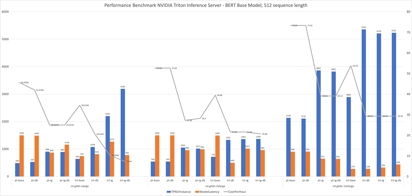
Results mostly validate the impact that was expected of different performance optimization features:
- TensorRT compilation has the most reliable impact across all instance types. Transactions per minute per instance increased by 30–35%, with a consistent cost reduction of approximately 25% when compared to the TensorRT engine’s performance to the default PyTorch BERT (
pt-base). The increased performance of the TensorRT engine is compounded upon and exploited by the other tested performance tuning features. - Loading two models on each GPU (instance group) almost strictly doubled all measured metrics. Invocations per minute per instance increased approximately 80–90%, yielding a cost reduction in the 50% range, almost as if we were using two GPUs. In fact, Amazon CloudWatch metrics for our experiments on g4dn.2xlarge (as an example) confirms that both CPU and GPU utilization double when we configure an instance group of two models.


Further performance and cost-optimization tips
The benchmark presented in this post just scratched the surface of the possible features and techniques that you can use with Triton to improve inference performance. These range from data preprocessing techniques, such as sending binary payloads to the model server or payloads with bigger batches, to native Triton features, such as the following:
- Model warmup, which prevents initial, slow inference requests by completely initializing the model before the first inference request is received.
- Response cache, which caches repeated requests.
- Model ensembling, which enables you to create a pipeline of one or more models and the connection of input and output tensors between those models. This opens the possibility of adding preprocessing and postprocessing steps, or even inference with other models, to the processing flow for each request.
We expect to test and benchmark these techniques and features in a future post, so stay tuned!
Conclusion
In this post, we explored a few parameters that you can use to maximize the performance of your SageMaker real-time endpoint for serving PyTorch BERT models with Triton Inference Server. We used SageMaker Inference Recommender to perform the benchmarking tests to fine-tune these parameters. These parameters are in essence related to TensorRT-based model optimization, leading to almost 50% improvement in response times compared to the non-optimized version. Additionally, running models concurrently and using dynamic batching of Triton led to almost a 70% increase in throughput. Fine-tuning these parameters led to an overall reduction of inference cost as well.
The best way to derive the correct values is through experimentation. However, to start building empirical knowledge on performance tuning and optimization, you can observe the combinations of different Triton-related parameters and their effect on performance across ML models and SageMaker ML instances.
SageMaker provides the tools to remove the undifferentiated heavy lifting from each stage of the ML lifecycle, thereby facilitating the rapid experimentation and exploration needed to fully optimize your model deployments.
You can find the notebook used for load testing and deployment on GitHub. You can update Triton configurations and SageMaker Inference Recommender settings to best fit your use case to achieve cost-effective and best-performing inference workloads.
About the Authors
 Vikram Elango is an AI/ML Specialist Solutions Architect at Amazon Web Services, based in Virginia USA. Vikram helps financial and insurance industry customers with design, thought leadership to build and deploy machine learning applications at scale. He is currently focused on natural language processing, responsible AI, inference optimization and scaling ML across the enterprise. In his spare time, he enjoys traveling, hiking, cooking and camping with his family.
 João Moura is an AI/ML Specialist Solutions Architect at Amazon Web Services. He mostly focuses on NLP use-cases and helping customers optimize Deep Learning model training and deployment. He is also an active proponent of low-code ML solutions and ML-specialized hardware.
 Mohan Gandhi is a Senior Software Engineer at AWS. He has been with AWS for the last 9 years and has worked on various AWS services like EMR, EFA and RDS on Outposts. Currently, he is focused on improving the SageMaker Inference Experience. In his spare time, he enjoys hiking and running marathons.
 Dhawal Patel is a Principal Machine Learning Architect at AWS. He has worked with organizations ranging from large enterprises to mid-sized startups on problems related to distributed computing, and Artificial Intelligence. He focuses on Deep learning including NLP and Computer Vision domains. He helps customers achieve high performance model inference on SageMaker.
 Santosh Bhavani is a Senior Technical Product Manager with the Amazon SageMaker Elastic Inference team. He focuses on helping SageMaker customers accelerate model inference and deployment. In his spare time, he enjoys traveling, playing tennis, and drinking lots of Pu’er tea.
 Jiahong Liu is a Solution Architect on the Cloud Service Provider team at NVIDIA. He assists clients in adopting machine learning and AI solutions that leverage NVIDIA accelerated computing to address their training and inference challenges. In his leisure time, he enjoys origami, DIY projects, and playing basketball.
Build a corporate credit ratings classifier using graph machine learning in Amazon SageMaker JumpStart
Today, we’re releasing a new solution for financial graph machine learning (ML) in Amazon SageMaker JumpStart. JumpStart helps you quickly get started with ML and provides a set of solutions for the most common use cases that can be trained and deployed with just a few clicks.
The new JumpStart solution (Graph-Based Credit Scoring) demonstrates how to construct a corporate network from SEC filings (long-form text data), combine this with financial ratios (tabular data), and use graph neural networks (GNNs) to build credit rating prediction models. In this post, we explain how you can use this fully customizable solution for credit scoring, so you can accelerate your graph ML journey. Graph ML is becoming a fruitful area for financial ML because it enables the use of network data in conjunction with traditional tabular datasets. For more information, see Amazon at WSDM: The future of graph neural networks.
Solution overview
You can improve credit scoring by exploiting data on business linkages, for which you may construct a graph, denoted as CorpNet (short for corporate network) in this solution. You can then apply graph ML classification using GNNs on this graph and a tabular feature set for the nodes, to see if you can build a better ML model by further exploiting the information in network relationships. Therefore, this solution offers a template for business models that exploit network data, such as using supply chain relationship graphs, social network graphs, and more.
The solution develops several new artifacts by constructing a corporate network and generating synthetic financial data, and combines both forms of data to create models using graph ML.
The solution shows how to construct a network of connected companies using the MD&A section from SEC 10-K/Q filings. Companies with similar forward-looking statements are likely to be connected for credit events. These connections are represented in a graph. For graph node features, the solution uses the variables in the Altman Z-score model and the industry category of each firm. These are provided in a synthetic dataset made available for demonstration purposes. The graph data and tabular data are used to fit a rating classifier using GNNs. For illustrative purposes, we compare the performance of models with and without the graph information.
Use the Graph-Based Credit Scoring solution
To start using JumpStart, see Getting started with Amazon SageMaker. The JumpStart card for the Graph-Based Credit Scoring solution is available through Amazon SageMaker Studio.

- Choose the model card, then choose Launch to initiate the solution.

The solution generates a model for inference and an endpoint to use with a notebook.
- Wait until they’re ready and the status shows as
Complete. - Choose Open Notebook to open the first notebook, which is for training and endpoint deployment.

You can work through this notebook to learn how to use this solution and then modify it for other applications on your own data. The solution comes with synthetic data and uses a subset of it to exemplify the steps needed to train the model, deploy it to an endpoint, and then invoke the endpoint for inference. The notebook also contains code to deploy an endpoint of your own.
- To open the second notebook (used for inference), choose Use Endpoint in Notebook next to the endpoint artifact.
In this notebook, you can see how to prepare the data to invoke the example endpoint to perform inference on a batch of examples.
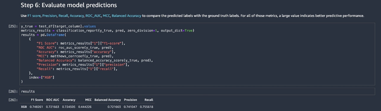
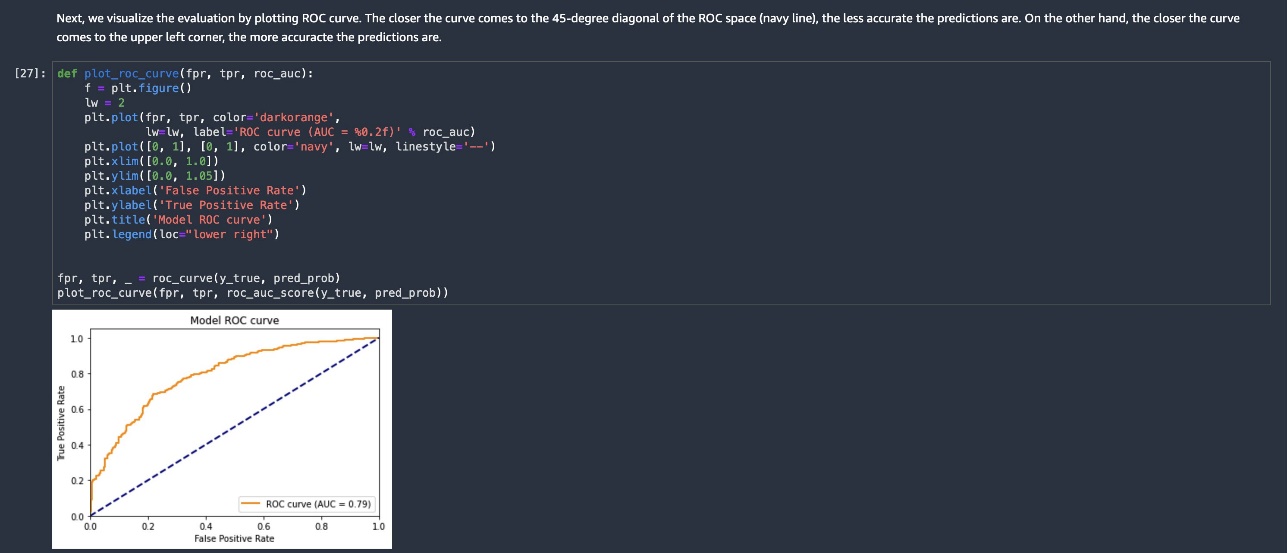
The endpoint returns predicted ratings, which are used to assess model performance, as shown in the following screenshot of the last code block of the inference notebook.
You can use this solution as a template for a graph-enhanced credit rating model. You’re not restricted to the feature set in this example—you can change both the graph data and tabular data for your own use case. The extent of code changes required is minimal. We recommend working through our template example to understand the structure of the solution, and then modify it as needed.
This solution is for demonstrative purposes only. It is not financial advice and should not be relied on as financial or investment advice. The associated notebooks, including the trained model, use synthetic data, and are not intended for production use. Although text from SEC filings is used, the financial data is synthetically and randomly generated and has no relation to any company’s true financials. Therefore, the synthetically generated ratings also don’t have any relation to any real company’s true rating.
Data used in the solution
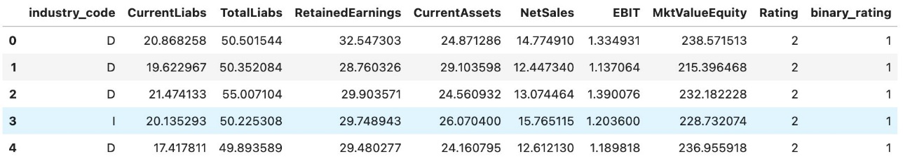
The dataset has synthetic tabular data such as various accounting ratios (numerical) and industry codes (categorical). The dataset has 𝑁=3286 rows. Rating labels are also added. These are the node features to be used with graph ML.
The dataset also contains a corporate graph, which is undirected and unweighted. This solution allows you to adjust the structure of the graph by varying the way in which links are included. Each company in the tabular dataset is represented by a node in the corporate graph. The function construct_network_data() helps construct the graph, which comprises lists of source nodes and destination nodes.
Rating labels are used for classification using GNNs, which can be multi-category for all ratings or binary, divided between investment grade (AAA, AA, A, BBB) and non-investment grade (BB, B, CCC, CC, C, D). D here stands for defaulted.
The complete code to read in the data and run the solution is provided in the solution notebook. The following screenshot shows the structure of the synthetic tabular data.
The graph information is passed in to the Deep Graph Library and combined with the tabular data to undertake graph ML. If you bring your own graph, simply supply it as a set of source nodes and destination nodes.
Model training
For comparison, we first train a model only on tabular data using AutoGluon, mimicking the traditional approach to credit rating of companies. We then add in the graph data and use GNNs for training. Full details are provided in the notebook, and a brief overview is offered in this post. The notebook also offers a quick overview of graph ML with selected references.
Training the GNN is undertaken as follows. We use an adaptation of the GraphSAGE model implemented in the Deep Graph Library.
- Read in graph data from Amazon Simple Storage Service (Amazon S3) and create the source and destination node lists for CorpNet.
- Read in the graph node feature sets (train and test). Normalize the data as required.
- Set tunable hyperparameters. Call the specialized graph ML container running PyTorch to fit the GNN without hyperparameter optimization (HPO).
- Repeat graph ML with HPO.
To make implementation straightforward and stable, we run model training in a container using the following code (the setup code prior to this training code is in the solution notebook):
The current training process is undertaken in a transductive setting, where the features of the test dataset (not including the target column) are used to construct the graph and therefore the test nodes are included in the training process. At the end of training, the predictions on the test dataset are generated and saved in output_location in the S3 bucket.
Even though the training is transductive, the labels of the test dataset aren’t used for training, and our exercise is aimed at predicting these labels using node embeddings for the test dataset nodes. An important feature of GraphSAGE is that inductive learning on new observations that aren’t part of the graph is also possible, though not exploited in this solution.
Hyperparameter optimization
This solution is further extended by conducting HPO on the GNN. This is done within SageMaker. See the following code:
We then set up the training objective, to maximize the F1 score in this case:
Establish the chosen environment and training resources on SageMaker:
Finally, run the training job with hyperparameter optimization:
Results
The inclusion of network data and hyperparameter optimization yields improved results. The performance metrics in the following table demonstrate the benefit of adding in CorpNet to standard tabular datasets used for credit scoring.
The results for AutoGluon don’t use the graph, only the tabular data. When we add in the graph data and use HPO, we get a material gain in performance.
| F1 Score | ROC AUC | Accuracy | MCC | Balanced Accuracy | Precision | Recall | |
| AutoGluon | 0.72 | 0.74323 | 0.68037 | 0.35233 | 0.67323 | 0.68528 | 0.75843 |
| GCN Without HPO | 0.64 | 0.84498 | 0.69406 | 0.45619 | 0.71154 | 0.88177 | 0.50281 |
| GCN With HPO | 0.81 | 0.87116 | 0.78082 | 0.563 | 0.77081 | 0.75119 | 0.89045 |
(Note: MCC is the Matthews Correlation Coefficient; https://en.wikipedia.org/wiki/Phi_coefficient.)
Clean up
After you’re done using this notebook, delete the model artifacts and other resources to avoid incurring further charges. You need to manually delete resources that you may have created while running the notebook, such as S3 buckets for model artifacts, training datasets, processing artifacts, and Amazon CloudWatch log groups.
Summary
In this post, we introduced a graph-based credit scoring solution in JumpStart to help you accelerate your graph ML journey. The notebook provides a pipeline that you can modify and exploit graphs with existing tabular models to obtain better performance.
To get started, you can find the Graph-Based Credit Scoring solution in JumpStart in SageMaker Studio.
About the Authors
 Dr. Sanjiv Das is an Amazon Scholar and the Terry Professor of Finance and Data Science at Santa Clara University. He holds post-graduate degrees in Finance (M.Phil and Ph.D. from New York University) and Computer Science (M.S. from UC Berkeley), and an MBA from the Indian Institute of Management, Ahmedabad. Prior to being an academic, he worked in the derivatives business in the Asia-Pacific region as a Vice President at Citibank. He works on multimodal machine learning in the area of financial applications.
 Dr. Xin Huang is an Applied Scientist for Amazon SageMaker JumpStart and Amazon SageMaker built-in algorithms. He focuses on developing scalable machine learning algorithms. His research interests are in the areas of natural language processing, deep learning on tabular data, and robust analysis of non-parametric space-time clustering.
 Soji Adeshina is an Applied Scientist at AWS, where he develops graph neural network-based models for machine learning on graphs tasks with applications to fraud and abuse, knowledge graphs, recommender systems, and life sciences. In his spare time, he enjoys reading and cooking.
 Patrick Yang is a Software Development Engineer at Amazon SageMaker. He focuses on building machine learning tools and products for customers.