Monthly Archives: July 2022

Machine learning (ML) is disrupting a lot of industries at an unprecedented pace. The healthcare and life sciences (HCLS) industry has been going through a rapid evolution in recent years embracing ML across a multitude of use cases for delivering quality care and improving patient outcomes.

In a typical ML lifecycle, data engineers and scientists spend the majority of their time on the data preparation and feature engineering steps before even getting started with the process of model building and training. Having a tool that can lower the barrier to entry for data preparation, thereby improving productivity, is a highly desirable ask for these personas. Amazon SageMaker Data Wrangler is purpose built by AWS to reduce the learning curve and enable data practitioners to accomplish data preparation, cleaning, and feature engineering tasks in less effort and time. It offers a GUI interface with many built-in functions and integrations with other AWS services such as Amazon Simple Storage Service (Amazon S3) and Amazon SageMaker Feature Store, as well as partner data sources including Snowflake and Databricks.

In this post, we demonstrate how to use Data Wrangler to prepare healthcare data for training a model to predict heart failure, given a patient’s demographics, prior medical conditions, and lab test result history.

Solution overview

The solution consists of the following steps:

1. Acquire a healthcare dataset as input to Data Wrangler.
2. Use Data Wrangler’s built-in transformation functions to transform the dataset. This includes drop columns, featurize data/time, join datasets, impute missing values, encode categorical variables, scale numeric values, balance the dataset, and more.
3. Use Data Wrangler’s custom transform function (Pandas or PySpark code) to supplement additional transformations required beyond the built-in transformations and demonstrate the extensibility of Data Wrangler. This includes filter rows, group data, form new dataframes based on conditions, and more.
4. Use Data Wrangler’s built-in visualization functions to perform visual analysis. This includes target leakage, feature correlation, quick model, and more.
5. Use Data Wrangler’s built-in export options to export the transformed dataset to Amazon S3.
6. Launch a Jupyter notebook to use the transformed dataset in Amazon S3 as input to train a model.

Generate a dataset

Now that we have settled on the ML problem statement, we first set our sights on acquiring the data we need. Research studies such as Heart Failure Prediction may provide data that’s already in good shape. However, we often encounter scenarios where the data is quite messy and requires joining, cleansing, and several other transformations that are very specific to the healthcare domain before it can be used for ML training. We want to find or generate data that is messy enough and walk you through the steps of preparing it using Data Wrangler. With that in mind, we picked Synthea as a tool to generate synthetic data that fits our goal. Synthea is an open-source synthetic patient generator that models the medical history of synthetic patients. To generate your dataset, complete the following steps:

1. Follow the instructions as per the quick start documentation to create an Amazon SageMaker Studio domain and launch Studio.
   This is a prerequisite step. It is optional if Studio is already set up in your account.
2. After Studio is launched, on the Launcher tab, choose System terminal.
   This launches a terminal session that gives you a command line interface to work with.
   
3. To install Synthea and generate the dataset in CSV format, run the following commands in the launched terminal session:

   $ sudo yum install -y java-1.8.0-openjdk-devel
   $ export JAVA_HOME=/usr/lib/jvm/jre-1.8.0-openjdk.x86_64
   $ export PATH=$JAVA_HOME/bin:$PATH
   $ git clone https://github.com/synthetichealth/synthea
   $ git checkout v3.0.0
   $ cd synthea
   $ ./run_synthea --exporter.csv.export=true -p 10000

We supply a parameter to generate the datasets with a population size of 10,000. Note the size parameter denotes the number of alive members of the population. Additionally, Synthea also generates data for dead members of the population which might add a few extra data points on top of the specified sample size.

Wait until the data generation is complete. This step usually takes around an hour or less. Synthea generates multiple datasets, including patients, medications, allergies, conditions, and more. For this post, we use three of the resulting datasets:

• patients.csv – This dataset is about 3.2 MB and contains approximately 11,000 rows of patient data (25 columns including patient ID, birthdate, gender, address, and more)
• conditions.csv – This dataset is about 47 MB and contains approximately 370,000 rows of medical condition data (six columns including patient ID, condition start date, condition code, and more)
• observations.csv – This dataset is about 830 MB and contains approximately 5 million rows of observation data (eight columns including patient ID, observation date, observation code, value, and more)

There is a one-to-many relationship between the patients and conditions datasets. There is also a one-to-many relationship between the patients and observations datasets. For a detailed data dictionary, refer to CSV File Data Dictionary.

4. To upload the generated datasets to a source bucket in Amazon S3, run the following commands in the terminal session:

   $ cd ./output/csv
   $ aws s3 sync . s3://<source bucket name>/

Launch Data Wrangler

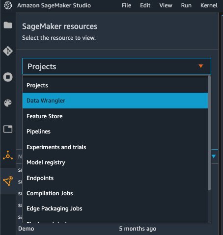
Choose SageMaker resources in the navigation page in Studio and on the Projects menu, choose Data Wrangler to create a Data Wrangler data flow. For detailed steps how to launch Data Wrangler from within Studio, refer to Get Started with Data Wrangler.

Import data

To import your data, complete the following steps:

1. Choose Amazon S3 and locate the patients.csv file in the S3 bucket.
2. In the Details pane, choose First K for Sampling.
3. Enter 1100 for Sample size.
   In the preview pane, Data Wrangler pulls the first 100 rows from the dataset and lists them as a preview.
4. Choose Import.
   Data Wrangler selects the first 1,100 patients from the total patients (11,000 rows) generated by Synthea and imports the data. The sampling approach lets Data Wrangler only process the sample data. It enables us to develop our data flow with a smaller dataset, which results in quicker processing and a shorter feedback loop. After we create the data flow, we can submit the developed recipe to a SageMaker processing job to horizontally scale out the processing for the full or larger dataset in a distributed fashion.
   
5. Repeat this process for the conditions and observations datasets.
   1. For the conditions dataset, enter 37000 for Sample size, which is 1/10 of the total 370,000 rows generated by Synthea.
   2. For the observations dataset, enter 500000 for Sample size, which is 1/10 of the total observations 5 million rows generated by Synthea.

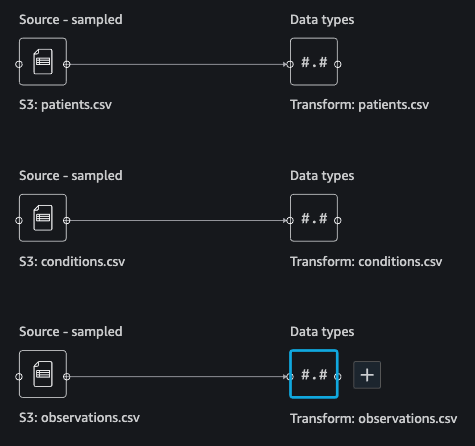
You should see three datasets as shown in the following screenshot.

Transform the data

Data transformation is the process of changing the structure, value, or format of one or more columns in the dataset. The process is usually developed by a data engineer and can be challenging for people with a smaller data engineering skillset to decipher the logic proposed for the transformation. Data transformation is part of the broader feature engineering process, and the correct sequence of steps is another important criterion to keep in mind while devising such recipes.

Data Wrangler is designed to be a low-code tool to reduce the barrier of entry for effective data preparation. It comes with over 300 preconfigured data transformations for you to choose from without writing a single line of code. In the following sections, we see how to transform the imported datasets in Data Wrangler.

Drop columns in patients.csv

We first drop some columns from the patients dataset. Dropping redundant columns removes non-relevant information from the dataset and helps us reduce the amount of computing resources required to process the dataset and train a model. In this section, we drop columns such as SSN or passport number based on common sense that these columns have no predictive value. In other words, they don’t help our model predict heart failure. Our study is also not concerned about other columns such as birthplace or healthcare expenses’ influence to a patient’s heart failure, so we drop them as well. Redundant columns can also be identified by running the built-in analyses like target leakage, feature correlation, multicollinearity, and more, which are built into Data Wrangler. For more details on the supported analyses types, refer to Analyze and Visualize. Additionally, you can use the Data Quality and Insights Report to perform automated analyses on the datasets to arrive at a list of redundant columns to eliminate.

1. Choose the plus sign next to Data types for the patients.csv dataset and choose Add transform.
   
2. Choose Add step and choose Manage columns.
   
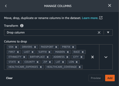
3. For Transform¸ choose Drop column.
4. For Columns to drop, choose the following columns:
   1. SSN
   2. DRIVERS
   3. PASSPORT
   4. PREFIX
   5. FIRST
   6. LAST
   7. SUFFIX
   8. MAIDEN
   9. RACE
   10. ETHNICITY
   11. BIRTHPLACE
   12. ADDRESS
   13. CITY
   14. STATE
   15. COUNTY
   16. ZIP
   17. LAT
   18. LON
   19. HEALTHCARE_EXPENSES
   20. HEALTHCARE_COVERAGE
5. Choose Preview to review the transformed dataset, then choose Add.
   
   You should see the step Drop column in your list of transforms.
   

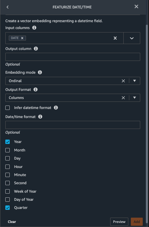
Featurize date/time in patients.csv

Now we use the Featurize date/time function to generate the new feature Year from the BIRTHDATE column in the patients dataset. We use the new feature in a subsequent step to calculate a patient’s age at the time of observation takes place.

1. In the Transforms pane of your Drop column page for the patients dataset, choose Add step.
2. Choose the Featurize date/time transform.
   
3. Choose Extract columns.
4. For Input columns, add the column BIRTHDATE.
5. Select Year and deselect Month, Day, Hour, Minute, Second.
   
   
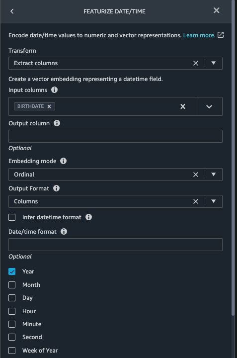
6. Choose Preview, then choose Add.

Add transforms in observations.csv

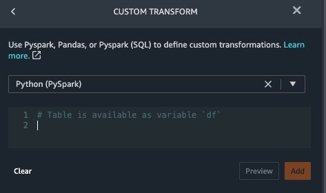
Data Wrangler supports custom transforms using Python (user-defined functions), PySpark, Pandas, or PySpark (SQL). You can choose your transform type based on your familiarity with each option and preference. For the latter three options, Data Wrangler exposes the variable df for you to access the dataframe and apply transformations on it. For a detailed explanation and examples, refer to Custom Transforms. In this section, we add three custom transforms to the observations dataset.

1. Add a transform to observations.csv and drop the DESCRIPTION column.
   
2. Choose Preview, then choose Add.
3. In the Transforms pane, choose Add step and choose Custom transform.
4. On the drop-down menu, choose Python (Pandas).
   
5. Enter the following code:

   df = df[df["CODE"].isin(['8867-4','8480-6','8462-4','39156-5','777-3'])]

   These are LONIC codes that correspond to the following observations we’re interested in using as features for predicting heart failure:

   heart rate: 8867-4
   systolic blood pressure: 8480-6
   diastolic blood pressure: 8462-4
   body mass index (BMI): 39156-5
   platelets [#/volume] in Blood: 777-3

6. Choose Preview, then choose Add.
7. Add a transform to extract Year and Quarter from the DATE column.
   
8. Choose Preview, then choose Add.
9. Choose Add step and choose Custom transform.
10. On the drop-down menu, choose Python (PySpark).
    
    The five types of observations may not always be recorded on the same date. For example, a patient may visit their family doctor on January 21 and have their systolic blood pressure, diastolic blood pressure, heart rate, and body mass index measured and recorded. However, a lab test that includes platelets may be done at a later date on February 2. Therefore, it’s not always possible to join dataframes by the observation date. Here we join dataframes on a coarse granularity at the quarter basis.
11. Enter the following code:

    from pyspark.sql.functions import col
    
    systolic_df = (
        df.select("patient", "DATE_year", "DATE_quarter", "value")
                       .withColumnRenamed("value", "systolic")
                       .filter((col("code") == "8480-6"))
      )
    
    diastolic_df = (
        df.select("patient", "DATE_year", "DATE_quarter", "value")
                       .withColumnRenamed('value', 'diastolic')
                       .filter((col("code") == "8462-4"))
        )
    
    hr_df = (
        df.select("patient", "DATE_year", "DATE_quarter", "value")
                       .withColumnRenamed('value', 'hr')
                       .filter((col("code") == "8867-4"))
        )
    
    bmi_df = (
        df.select("patient", "DATE_year", "DATE_quarter", "value")
                       .withColumnRenamed('value', 'bmi')
                       .filter((col("code") == "39156-5"))
        )
    
    platelets_df = (
        df.select("patient", "DATE_year", "DATE_quarter", "value")
                       .withColumnRenamed('value', 'platelets')
                       .filter((col("code") == "777-3"))
        )
    
    df = (
        systolic_df.join(diastolic_df, ["patient", "DATE_year", "DATE_quarter"])
                                .join(hr_df, ["patient", "DATE_year", "DATE_quarter"])
                                .join(bmi_df, ["patient", "DATE_year", "DATE_quarter"])
                                .join(platelets_df, ["patient", "DATE_year", "DATE_quarter"])
    )

12. Choose Preview, then choose Add.
13. Choose Add step, then choose Manage rows.
14. For Transform, choose Drop duplicates.
    
15. Choose Preview, then choose Add.
16. Choose Add step and choose Custom transform.
17. On the drop-down menu, choose Python (Pandas).
18. Enter the following code to take an average of data points that share the same time value:

    import pandas as pd
    df.loc[:, df.columns != 'patient']=df.loc[:, df.columns != 'patient'].apply(pd.to_numeric)
    df = df.groupby(['patient','DATE_year','DATE_quarter']).mean().round(0).reset_index()

19. Choose Preview, then choose Add.
    

Join patients.csv and observations.csv

In this step, we showcase how to effectively and easily perform complex joins on datasets without writing any code via Data Wrangler’s powerful UI. To learn more about the supported types of joins, refer to Transform Data.

1. To the right of Transform: patients.csv, choose the plus sign next to Steps and choose Join.
   You can see the transformed patients.csv file listed under Datasets in the left pane.
   
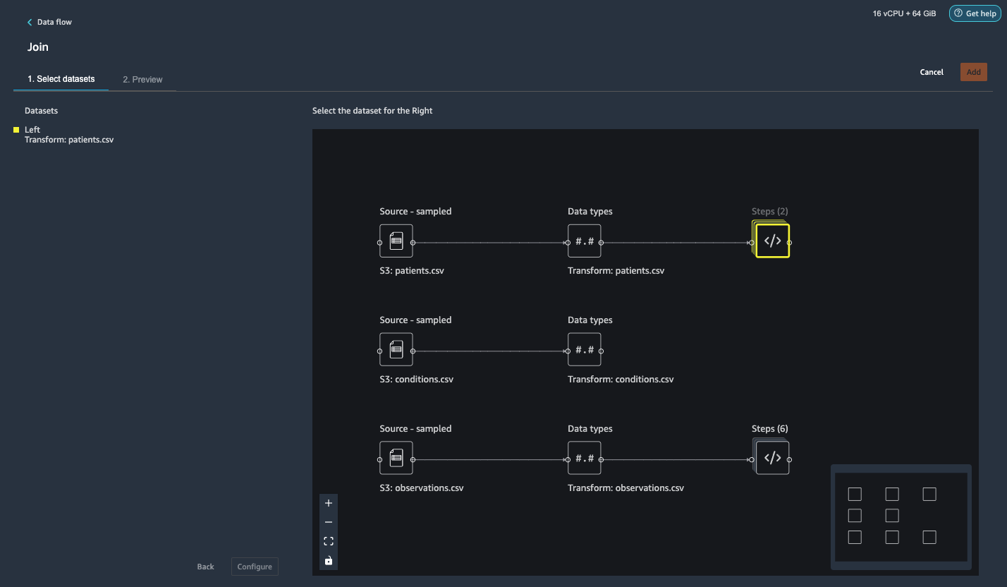
2. To the right of Transform: observations.csv, click on the Steps to initiate the join operation.
   The transformed observations.csv file is now listed under Datasets in the left pane.
   
3. Choose Configure.
4. For Join Type, choose Inner.
5. For Left, choose Id.
6. For Right, choose patient.
7. Choose Preview, then choose Add.
   

Add a custom transform to the joined datasets

In this step, we calculate a patient’s age at the time of observation. We also drop columns that are no longer needed.

1. Choose the plus sign next to 1st Join and choose Add transform.
2. Add a custom transform in Pandas:

   df['age'] = df['DATE_year'] - df['BIRTHDATE_year']
   df = df.drop(columns=['BIRTHDATE','DEATHDATE','BIRTHDATE_year','patient'])

3. Choose Preview, then choose Add.

Add custom transforms to conditions.csv

1. Choose the plus sign next to Transform: conditions.csv and choose Add transform.
2. Add a custom transform in Pandas:

   df = df[df["CODE"].isin(['84114007', '88805009', '59621000', '44054006', '53741008', '449868002', '49436004'])]
   df = df.drop(columns=['DESCRIPTION','ENCOUNTER','STOP'])

Note: As we demonstrated earlier, you can drop columns either using custom code or using the built-in transformations provided by Data Wrangler. Custom transformations within Data Wrangler provides the flexibility to bring your own transformation logic in the form of code snippets in the supported frameworks. These snippets can later be searched and applied if needed.

The codes in the preceding transform are SNOMED-CT codes that correspond to the following conditions. The heart failure or chronic congestive heart failure condition becomes the label. We use the remaining conditions as features for predicting heart failure. We also drop a few columns that are no longer needed.

Heart failure: 84114007
Chronic congestive heart failure: 88805009
Hypertension: 59621000
Diabetes: 44054006
Coronary Heart Disease: 53741008
Smokes tobacco daily: 449868002
Atrial Fibrillation: 49436004

3. Next, let’s add a custom transform in PySpark:

   from pyspark.sql.functions import col, when
   
   heartfailure_df = (
       df.select("patient", "start")
                         .withColumnRenamed("start", "heartfailure")
                      .filter((col("code") == "84114007") | (col("code") == "88805009"))
     )
   
   hypertension_df = (
       df.select("patient", "start")
                      .withColumnRenamed("start", "hypertension")
                      .filter((col("code") == "59621000"))
     )
   
   diabetes_df = (
       df.select("patient", "start")
                      .withColumnRenamed("start", "diabetes")
                      .filter((col("code") == "44054006"))
     )
   
   coronary_df = (
       df.select("patient", "start")
                      .withColumnRenamed("start", "coronary")
                      .filter((col("code") == "53741008"))
     )
   
   smoke_df = (
       df.select("patient", "start")
                      .withColumnRenamed("start", "smoke")
                      .filter((col("code") == "449868002"))
     )
   
   atrial_df = (
       df.select("patient", "start")
                      .withColumnRenamed("start", "atrial")
                      .filter((col("code") == "49436004"))
     )
   
   df = (
       heartfailure_df.join(hypertension_df, ["patient"], "leftouter").withColumn("has_hypertension", when(col("hypertension") < col("heartfailure"), 1).otherwise(0))
       .join(diabetes_df, ["patient"], "leftouter").withColumn("has_diabetes", when(col("diabetes") < col("heartfailure"), 1).otherwise(0))
       .join(coronary_df, ["patient"], "leftouter").withColumn("has_coronary", when(col("coronary") < col("heartfailure"), 1).otherwise(0))
       .join(smoke_df, ["patient"], "leftouter").withColumn("has_smoke", when(col("smoke") < col("heartfailure"), 1).otherwise(0))
       .join(atrial_df, ["patient"], "leftouter").withColumn("has_atrial", when(col("atrial") < col("heartfailure"), 1).otherwise(0))
   )

   We perform a left outer join to keep all entries in the heart failure dataframe. A new column has_xxx is calculated for each condition other than heart failure based on the condition’s start date. We’re only interested in medical conditions that were recorded prior to the heart failure and use them as features for predicting heart failure.

4. Add a built-in Manage columns transform to drop the redundant columns that are no longer needed:
   1. hypertension
   2. diabetes
   3. coronary
   4. smoke
   5. atrial
5. Extract Year and  Quarter from the heartfailure column.
   This matches the granularity we used earlier in the transformation of the observations dataset.
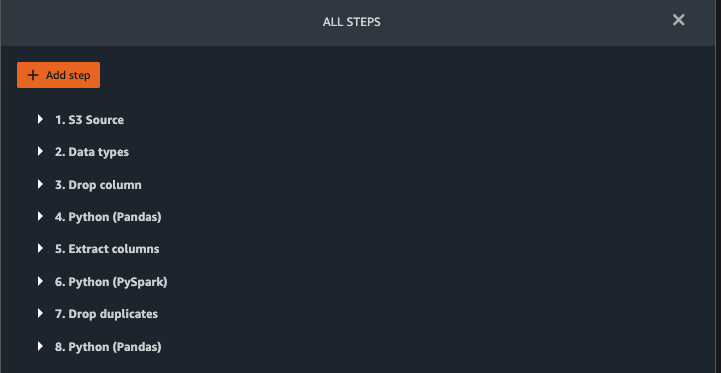
6. We should have a total of 6 steps for conditions.csv.
   

Join conditions.csv to the joined dataset

We now perform a new join to join the conditions dataset to the joined patients and observations dataset.

1. Choose Transform: 1st Join.
2. Choose the plus sign and choose Join.
3. Choose Steps next to Transform: conditions.csv.
   
4. Choose Configure.
5. For Join Type, choose Left outer.
6. For Left, choose Id.
7. For Right, choose patient.
8. Choose Preview, then choose Add.
   

Add transforms to the joined datasets

Now that we have all three datasets joined, let’s apply some additional transformations.

1. Add the following custom transform in PySpark so has_heartfailure becomes our label column:

   from pyspark.sql.functions import col, when
   df = (
       df.withColumn("has_heartfailure", when(col("heartfailure").isNotNull(), 1).otherwise(0))
   )

2. Add the following custom transformation in PySpark:

   from pyspark.sql.functions import col
   
   df = (
       df.filter(
         (col("has_heartfailure") == 0) | 
         ((col("has_heartfailure") == 1) & ((col("date_year") <= col("heartfailure_year")) | ((col("date_year") == col("heartfailure_year")) & (col("date_quarter") <= col("heartfailure_quarter")))))
       )
   )

   We’re only interested in observations recorded prior to when the heart failure condition is diagnosed and use them as features for predicting heart failure. Observations taken after heart failure is diagnosed may be affected by the medication a patient takes, so we want to exclude those ones.

3. Drop the redundant columns that are no longer needed:
   1. Id
   2. DATE_year
   3. DATE_quarter
   4. patient
   5. heartfailure
   6. heartfailure_year
   7. heartfailure_quarter
4. On the Analysis tab, for Analysis type¸ choose Table summary.
   A quick scan through the summary shows that the MARITAL column has missing data.
   
5. Choose the Data tab and add a step.
6. Choose Handle Missing.
7. For Transform, choose Fill missing.
8. For Input columns, choose MARITAL.
9. For Fill value, enter S.
   Our strategy here is to assume the patient is single if the marital status has missing value. You can have a different strategy.
   
10. Choose Preview, then choose Add.
11. Fill the missing value as 0 for has_hypertension, has_diabetes, has_coronary, has_smoke, has_atrial.

Marital and Gender are categorial variables. Data Wrangler has a built-in function to encode categorial variables.

12. Add a step and choose Encode categorial.
13. For Transform, choose One-hot encode.
14. For Input columns, choose MARITAL.
15. For Output style, choose Column.
    This output style produces encoded values in separate columns.
    
16. Choose Preview, then choose Add.
17. Repeat these steps for the Gender column.

The one-hot encoding splits the Marital column into Marital_M (married) and Marital_S (single), and splits the Gender column into Gender_M (male) and Gender_F (female). Because Marital_M and Marital_S are mutually exclusive (as are Gender_M and Gender_F), we can drop one column to avoid redundant features.

18. Drop Marital_S and Gender_F.

Numeric features such as systolic, heart rate, and age have different unit standards. For a linear regression-based model, we need to normalize these numeric features first. Otherwise, some features with higher absolute values may have an unwarranted advantage over other features with lower absolute values and result in poor model performance. Data Wrangler has the built-in transform Min-max scaler to normalize the data. For a decision tree-based classification model, normalization isn’t required. Our study is a classification problem so we don’t need to apply normalization. Imbalanced classes are a common problem in classification. Imbalance happens when the training dataset contains severely skewed class distribution. For example, when our dataset contains disproportionally more patients without heart failure than patients with heart failure, it can cause the model to be biased toward predicting no heart failure and perform poorly. Data Wrangler has a built-in function to tackle the problem.

19. Add a custom transform in Pandas to convert data type of columns from “object” type to numeric type:

    import pandas as pd
    df=df.apply(pd.to_numeric)

20. Choose the Analysis tab.
21. For Analysis type¸ choose Histogram.
22. For X axis, choose has_heartfailure.
23. Choose Preview.
    
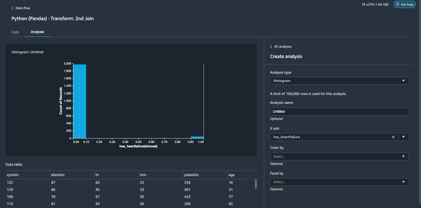
    It’s obvious that we have an imbalanced class (more data points labeled as no heart failure than data points labeled as heart failure).
24. Go back to the Data tab. Choose Add step and choose Balance data.
25. For Target column, choose has_heartfailure.
26. For Desired ratio, enter 1.
27. For Transform, choose SMOTE.
    
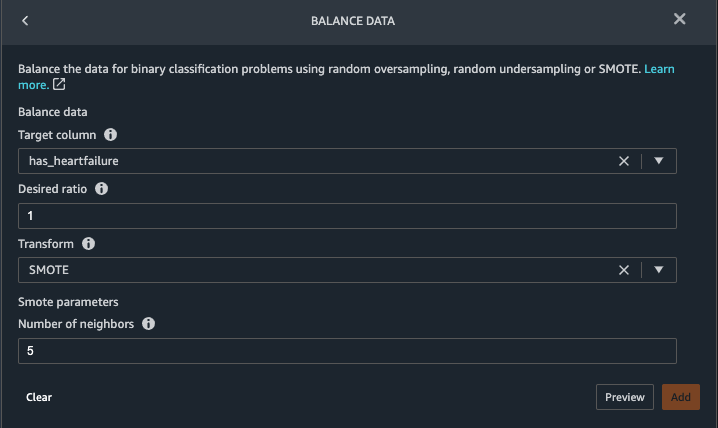
    SMOTE stands for Synthetic Minority Over-sampling Technique. It’s a technique to create new minority instances and add to the dataset to reach class balance. For detailed information, refer to SMOTE: Synthetic Minority Over-sampling Technique.
28. Choose Preview, then choose Add.
29. Repeat the histogram analysis in step 20-23. The result is a balanced class.
    

Visualize target leakage and feature correlation

Next, we’re going to perform a few visual analyses using Data Wrangler’s rich toolset of advanced ML-supported analysis types. First, we look at target leakage. Target leakage occurs when data in the training dataset is strongly correlated with the target label, but isn’t available in real-world data at inference time.

1. On the Analysis tab, for Analysis type¸ choose Target Leakage.
2. For Problem Type, choose classification.
3. For Target, choose has_heartfailure.
4. Choose Preview.
   
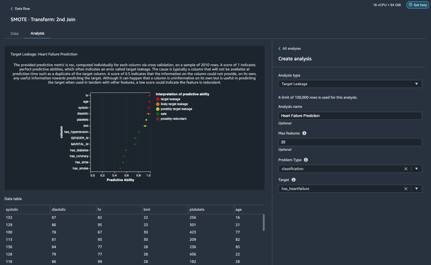
   Based on the analysis, hr is a target leakage. We’ll drop it in a subsequent step. age is flagged a target leakage. It’s reasonable to say that a patient’s age will be available during inference time, so we keep age as a feature. Systolic and diastolic are also flagged as likely target leakage. We expect to have the two measurements during inference time, so we keep them as features.
5. Choose Add to add the analysis.

Then, we look at feature correlation. We want to select features that are correlated with the target but are uncorrelated among themselves.

6. On the Analysis tab, for Analysis type¸ choose Feature Correlation.
7. For Correlation Type¸ choose linear.
8. Choose Preview.
   

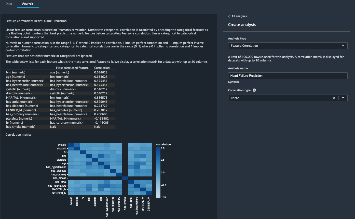
The coefficient scores indicate strong correlations between the following pairs:

• systolic and diastolic
• bmi and age
• has_hypertension and has_heartfailure (label)

For features that are strongly correlated, matrices are computationally difficult to invert, which can lead to numerically unstable estimates. To mitigate the correlation, we can simply remove one from the pair. We drop diastolic and bmi and keep systolic and age in a subsequent step.

Drop diastolic and bmi columns

Add additional transform steps to drop the hr, diastolic and bmi columns using the built-in transform.

Generate the Data Quality and Insights Report

AWS recently announced the new Data Quality and Insights Report feature in Data Wrangler. This report automatically verifies data quality and detects abnormalities in your data. Data scientists and data engineers can use this tool to efficiently and quickly apply domain knowledge to process datasets for ML model training. This step is optional. To generate this report on our datasets, complete the following steps:

1. On the Analysis tab, for Analysis type, choose Data Quality and Insights Report.
2. For Target column, choose has_heartfailure.
3. For Problem type, select Classification.
4. Choose Create.
   

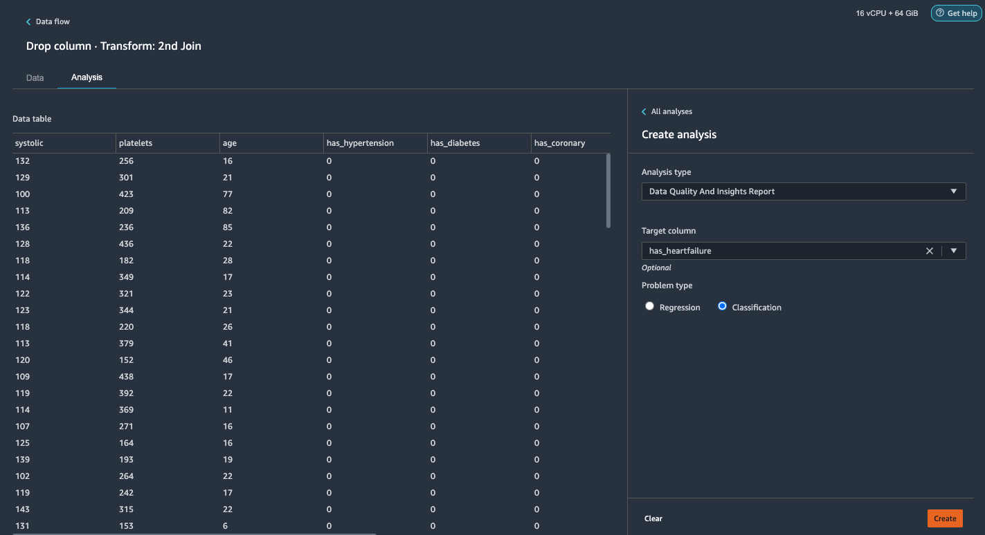
In a few minutes, it generates a report with a summary, visuals, and recommendations.

Generate a Quick Model analysis

We have completed our data preparation, cleaning, and feature engineering. Data Wrangler has a built-in function that provides a rough estimate of the expected predicted quality and the predictive power of features in our dataset.

1. On the Analysis tab, for Analysis type¸ choose Quick Model.
2. For Label, choose has_heartfailure.
3. Choose Preview.
   

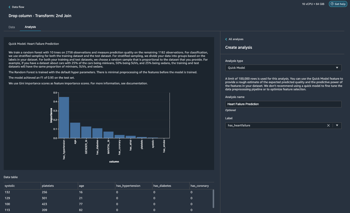
As per our Quick Model analysis, we can see the feature has_hypertension has the highest feature importance score among all features.

Export the data and train the model

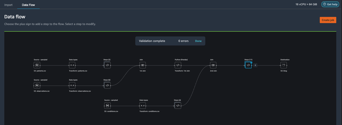
Now let’s export the transformed ML-ready features to a destination S3 bucket and scale the entire feature engineering pipeline we have created so far using the samples into the entire dataset in a distributed fashion.

1. Choose the plus sign next to the last box in the data flow and choose Add destination.
2. Choose Amazon S3.
   
3. Enter a Dataset name. For Amazon S3 location, choose a S3 bucket, then choose Add Destination.
4. Choose Create job to launch a distributed PySpark processing job to perform the transformation and output the data to the destination S3 bucket.
   
   Depending on the size of the datasets, this option lets us easily configure the cluster and horizontally scale in a no-code fashion. We don’t have to worry about partitioning the datasets or managing the cluster and Spark internals. All of this is automatically taken care for us by Data Wrangler.
5. On the left pane, choose Next, 2. Configure job.
   
   
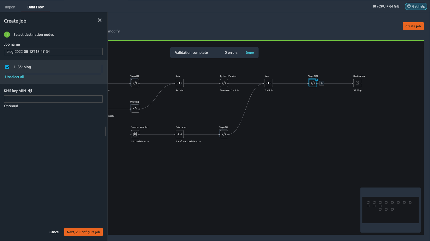
6. Then choose Run.
   

Alternatively, we can also export the transformed output to S3 via a Jupyter Notebook. With this approach, Data Wrangler automatically generates a Jupyter notebook with all the code needed to kick-off a processing job to apply the data flow steps (created using a sample) on the larger full dataset and use the transformed dataset as features to kick-off a training job later. The notebook code can be readily run with or without making changes. Let’s now walk through the steps on how to get this done via Data Wrangler’s UI.

1. Choose the plus sign next to the last step in the data flow and choose Export to.
2. Choose Amazon S3 (via Jupyter Notebook).
   
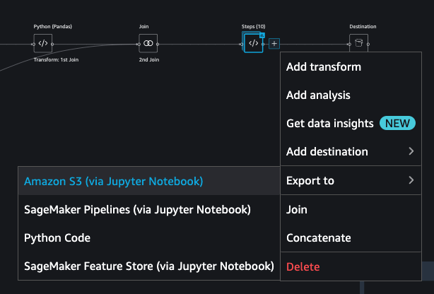
3. It automatically opens a new tab with a Jupyter notebook.
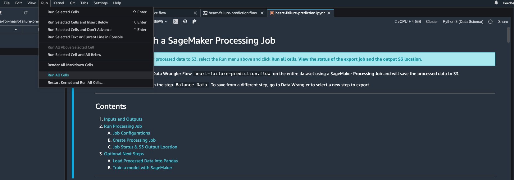
4. In the Jupyter notebook, locate the cell in the (Optional) Next Steps section and change run_optional_steps from False to True.
   The enabled optional steps in the notebook perform the following:
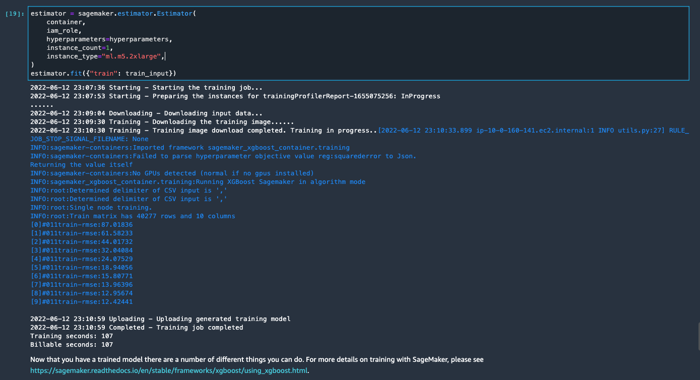
   • Train a model using XGBoost
     
5. Go back to the top of the notebook and on the Run menu, choose Run All Cells.

If you use the generated notebook as is, it launches a SageMaker processing job that scales out the processing across two m5.4xlarge instances to processes the full dataset on the S3 bucket. You can adjust the number of instances and instance types based on the dataset size and time you need to complete the job.

Wait until the training job from the last cell is complete. It generates a model in the SageMaker default S3 bucket.

The trained model is ready for deployment for either real-time inference or batch transformation. Note that we used synthetic data to demonstrate functionalities in Data Wrangler and used processed data for training model. Given that the data we used is synthetic, the inference result from the trained model is not meant for real-world medical condition diagnosis or substitution of judgment from medical practitioners.

You can also directly export your transformed dataset into Amazon S3 by choosing Export on top of the transform preview page. The direct export option only exports the transformed sample if sampling was enabled during the import. This option is best suited if you’re dealing with smaller datasets. The transformed data can also be ingested directly into a feature store. For more information, refer to Amazon SageMaker Feature Store. The data flow can also be exported as a SageMaker pipeline that can be orchestrated and scheduled as per your requirements. For more information, see Amazon SageMaker Pipelines.

Conclusion

In this post, we showed how to use Data Wrangler to process healthcare data and perform scalable feature engineering in a tool-driven, low-code fashion. We learned how to apply the built-in transformations and analyses aptly wherever needed, combining it with custom transformations to add even more flexibility to our data preparation workflow. We also walked through the different options for scaling out the data flow recipe via distributed processing jobs. We also learned how the transformed data can be easily used for training a model to predict heart failure.

There are many other features in Data Wrangler we haven’t covered in this post. Explore what’s possible in Prepare ML Data with Amazon SageMaker Data Wrangler and learn how to leverage Data Wrangler for your next data science or machine learning project.

About the Authors

Forrest Sun is a Senior Solution Architect with the AWS Public Sector team in Toronto, Canada. He has worked in the healthcare and finance industries for the past two decades. Outside of work, he enjoys camping with his family.

Arunprasath Shankar is an Artificial Intelligence and Machine Learning (AI/ML) Specialist Solutions Architect with AWS, helping global customers scale their AI solutions effectively and efficiently in the cloud. In his spare time, Arun enjoys watching sci-fi movies and listening to classical music.

Read More