Colin, CBO at DeepMind, discusses collaborations with Alphabet and how we integrate ethics, accountability, and safety into everything we do.Read More

A Multi-Axis Approach for Vision Transformer and MLP Models
Convolutional neural networks have been the dominant machine learning architecture for computer vision since the introduction of AlexNet in 2012. Recently, inspired by the evolution of Transformers in natural language processing, attention mechanisms have been prominently incorporated into vision models. These attention methods boost some parts of the input data while minimizing other parts so that the network can focus on small but important parts of the data. The Vision Transformer (ViT) has created a new landscape of model designs for computer vision that is completely free of convolution. ViT regards image patches as a sequence of words, and applies a Transformer encoder on top. When trained on sufficiently large datasets, ViT demonstrates compelling performance on image recognition.
While convolutions and attention are both sufficient for good performance, neither of them are necessary. For example, MLP-Mixer adopts a simple multi-layer perceptron (MLP) to mix image patches across all the spatial locations, resulting in an all-MLP architecture. It is a competitive alternative to existing state-of-the-art vision models in terms of the trade-off between accuracy and computation required for training and inference. However, both ViT and the MLP models struggle to scale to higher input resolution because the computational complexity increases quadratically with respect to the image size.
Today we present a new multi-axis approach that is simple and effective, improves on the original ViT and MLP models, can better adapt to high-resolution, dense prediction tasks, and can naturally adapt to different input sizes with high flexibility and low complexity. Based on this approach, we have built two backbone models for high-level and low-level vision tasks. We describe the first in “MaxViT: Multi-Axis Vision Transformer”, to be presented in ECCV 2022, and show it significantly improves the state of the art for high-level tasks, such as image classification, object detection, segmentation, quality assessment, and generation. The second, presented in “MAXIM: Multi-Axis MLP for Image Processing” at CVPR 2022, is based on a UNet-like architecture and achieves competitive performance on low-level imaging tasks including denoising, deblurring, dehazing, deraining, and low-light enhancement. To facilitate further research on efficient Transformer and MLP models, we have open-sourced the code and models for both MaxViT and MAXIM.
 |
| A demo of image deblurring using MAXIM frame by frame. |
Overview
Our new approach is based on multi-axis attention, which decomposes the full-size attention (each pixel attends to all the pixels) used in ViT into two sparse forms — local and (sparse) global. As shown in the figure below, the multi-axis attention contains a sequential stack of block attention and grid attention. The block attention works within non-overlapping windows (small patches in intermediate feature maps) to capture local patterns, while the grid attention works on a sparsely sampled uniform grid for long-range (global) interactions. The window sizes of grid and block attentions can be fully controlled as hyperparameters to ensure a linear computational complexity to the input size.
 |
| The proposed multi-axis attention conducts blocked local and dilated global attention sequentially followed by a FFN, with only a linear complexity. The pixels in the same colors are attended together. |
Such low-complexity attention can significantly improve its wide applicability to many vision tasks, especially for high-resolution visual predictions, demonstrating greater generality than the original attention used in ViT. We build two backbone instantiations out of this multi-axis attention approach – MaxViT and MAXIM, for high-level and low-level tasks, respectively.
MaxViT
In MaxViT, we first build a single MaxViT block (shown below) by concatenating MBConv (proposed by EfficientNet, V2) with the multi-axis attention. This single block can encode local and global visual information regardless of input resolution. We then simply stack repeated blocks composed of attention and convolutions in a hierarchical architecture (similar to ResNet, CoAtNet), yielding our homogenous MaxViT architecture. Notably, MaxViT is distinguished from previous hierarchical approaches as it can “see” globally throughout the entire network, even in earlier, high-resolution stages, demonstrating stronger model capacity on various tasks.
 |
| The meta-architecture of MaxViT. |
MAXIM
Our second backbone, MAXIM, is a generic UNet-like architecture tailored for low-level image-to-image prediction tasks. MAXIM explores parallel designs of the local and global approaches using the gated multi-layer perceptron (gMLP) network (patching-mixing MLP with a gating mechanism). Another contribution of MAXIM is the cross-gating block that can be used to apply interactions between two different input signals. This block can serve as an efficient alternative to the cross-attention module as it only employs the cheap gated MLP operators to interact with various inputs without relying on the computationally heavy cross-attention. Moreover, all the proposed components including the gated MLP and cross-gating blocks in MAXIM enjoy linear complexity to image size, making it even more efficient when processing high-resolution pictures.
Results
We demonstrate the effectiveness of MaxViT on a broad range of vision tasks. On image classification, MaxViT achieves state-of-the-art results under various settings: with only ImageNet-1K training, MaxViT attains 86.5% top-1 accuracy; with ImageNet-21K (14M images, 21k classes) pre-training, MaxViT achieves 88.7% top-1 accuracy; and with JFT (300M images, 18k classes) pre-training, our largest model MaxViT-XL achieves a high accuracy of 89.5% with 475M parameters.
 |
 |
| Performance comparison of MaxViT with state-of-the-art models on ImageNet-1K. Top: Accuracy vs. FLOPs performance scaling with 224×224 image resolution. Bottom: Accuracy vs. parameters scaling curve under ImageNet-1K fine-tuning setting. |
For downstream tasks, MaxViT as a backbone delivers favorable performance on a broad spectrum of tasks. For object detection and segmentation on the COCO dataset, the MaxViT backbone achieves 53.4 AP, outperforming other base-level models while requiring only about 60% the computational cost. For image aesthetics assessment, the MaxViT model advances the state-of-the-art MUSIQ model by 3.5% in terms of linear correlation with human opinion scores. The standalone MaxViT building block also demonstrates effective performance on image generation, achieving better FID and IS scores on the ImageNet-1K unconditional generation task with a significantly lower number of parameters than the state-of-the-art model, HiT.
The UNet-like MAXIM backbone, customized for image processing tasks, has also demonstrated state-of-the-art results on 15 out of 20 tested datasets, including denoising, deblurring, deraining, dehazing, and low-light enhancement, while requiring fewer or comparable number of parameters and FLOPs than competitive models. Images restored by MAXIM show more recovered details with less visual artifacts.
 |
| Visual results of MAXIM for image deblurring, deraining, and low-light enhancement. |
Summary
Recent works in the last two or so years have shown that ConvNets and Vision Transformers can achieve similar performance. Our work presents a unified design that takes advantage of the best of both worlds — efficient convolution and sparse attention — and demonstrates that a model built on top, namely MaxViT, can achieve state-of-the-art performance on a variety of vision tasks. More importantly, MaxViT scales well to very large data sizes. We also show that an alternative multi-axis design using MLP operators, MAXIM, achieves state-of-the-art performance on a broad range of low-level vision tasks.
Even though we present our models in the context of vision tasks, the proposed multi-axis approach can easily extend to language modeling to capture both local and global dependencies in linear time. Motivated by the work here, we expect that it is worthwhile to study other forms of sparse attention in higher-dimensional or multimodal signals such as videos, point clouds, and vision-language models.
We have open-sourced the code and models of MAXIM and MaxViT to facilitate future research on efficient attention and MLP models.
Acknowledgments
We would like to thank our co-authors: Hossein Talebi, Han Zhang, Feng Yang, Peyman Milanfar, and Alan Bovik. We would also like to acknowledge the valuable discussion and support from Xianzhi Du, Long Zhao, Wuyang Chen, Hanxiao Liu, Zihang Dai, Anurag Arnab, Sungjoon Choi, Junjie Ke, Mauricio Delbracio, Irene Zhu, Innfarn Yoo, Huiwen Chang, and Ce Liu.
Interspeech 2022
Apple Machine Learning Research
NVIDIA Hopper Sweeps AI Inference Benchmarks in MLPerf Debut
In their debut on the MLPerf industry-standard AI benchmarks, NVIDIA H100 Tensor Core GPUs set world records in inference on all workloads, delivering up to 4.5x more performance than previous-generation GPUs.
The results demonstrate that Hopper is the premium choice for users who demand utmost performance on advanced AI models.
Additionally, NVIDIA A100 Tensor Core GPUs and the NVIDIA Jetson AGX Orin module for AI-powered robotics continued to deliver overall leadership inference performance across all MLPerf tests: image and speech recognition, natural language processing and recommender systems.
The H100, aka Hopper, raised the bar in per-accelerator performance across all six neural networks in the round. It demonstrated leadership in both throughput and speed in separate server and offline scenarios.
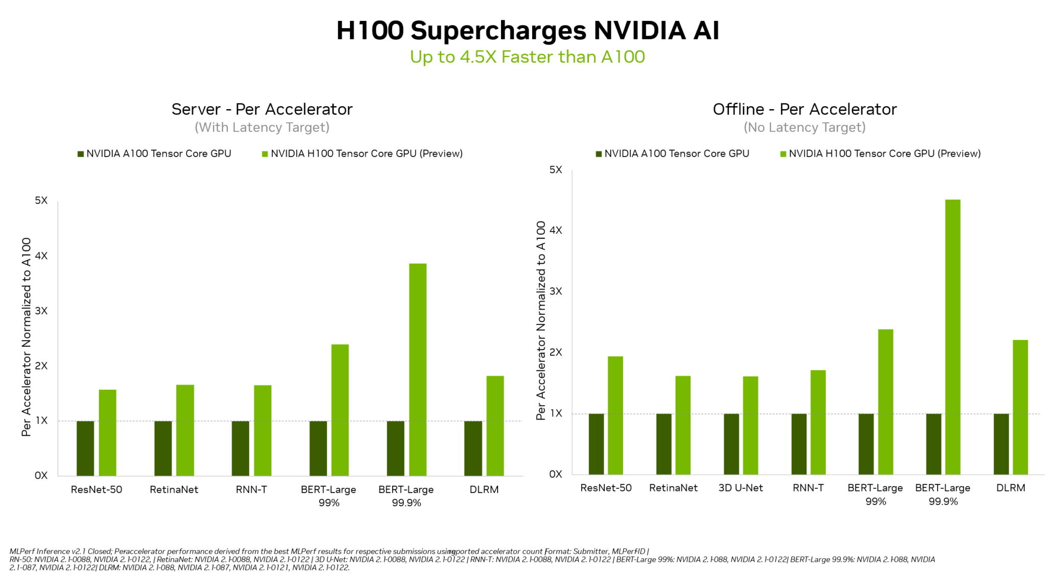
The NVIDIA Hopper architecture delivered up to 4.5x more performance than NVIDIA Ampere architecture GPUs, which continue to provide overall leadership in MLPerf results.
Thanks in part to its Transformer Engine, Hopper excelled on the popular BERT model for natural language processing. It’s among the largest and most performance-hungry of the MLPerf AI models.
These inference benchmarks mark the first public demonstration of H100 GPUs, which will be available later this year. The H100 GPUs will participate in future MLPerf rounds for training.
A100 GPUs Show Leadership
NVIDIA A100 GPUs, available today from major cloud service providers and systems manufacturers, continued to show overall leadership in mainstream performance on AI inference in the latest tests.
A100 GPUs won more tests than any submission in data center and edge computing categories and scenarios. In June, the A100 also delivered overall leadership in MLPerf training benchmarks, demonstrating its abilities across the AI workflow.
Since their July 2020 debut on MLPerf, A100 GPUs have advanced their performance by 6x, thanks to continuous improvements in NVIDIA AI software.
NVIDIA AI is the only platform to run all MLPerf inference workloads and scenarios in data center and edge computing.
Users Need Versatile Performance
The ability of NVIDIA GPUs to deliver leadership performance on all major AI models makes users the real winners. Their real-world applications typically employ many neural networks of different kinds.
For example, an AI application may need to understand a user’s spoken request, classify an image, make a recommendation and then deliver a response as a spoken message in a human-sounding voice. Each step requires a different type of AI model.
The MLPerf benchmarks cover these and other popular AI workloads and scenarios — computer vision, natural language processing, recommendation systems, speech recognition and more. The tests ensure users will get performance that’s dependable and flexible to deploy.
Users rely on MLPerf results to make informed buying decisions, because the tests are transparent and objective. The benchmarks enjoy backing from a broad group that includes Amazon, Arm, Baidu, Google, Harvard, Intel, Meta, Microsoft, Stanford and the University of Toronto.
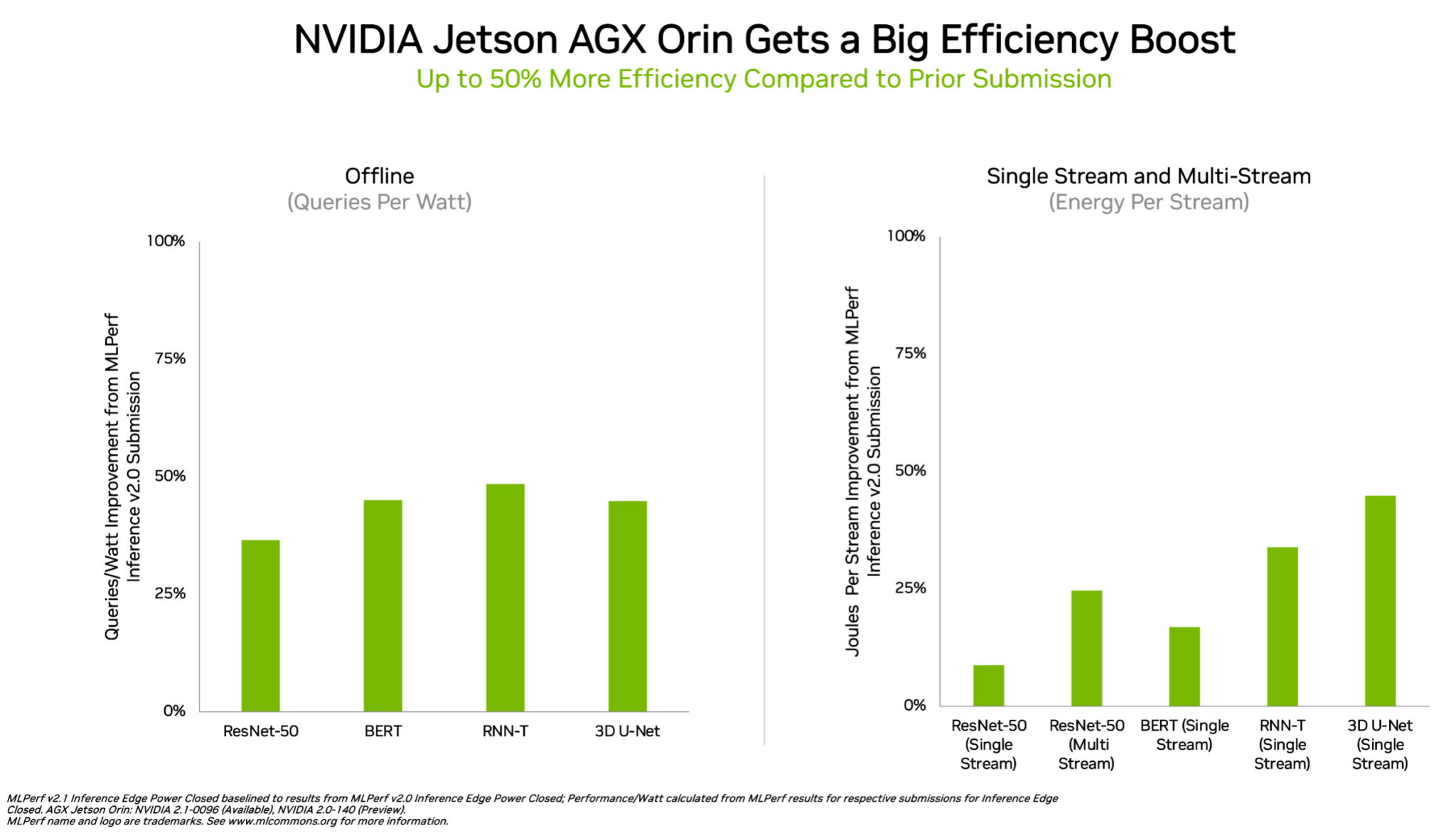
Orin Leads at the Edge
In edge computing, NVIDIA Orin ran every MLPerf benchmark, winning more tests than any other low-power system-on-a-chip. And it showed up to a 50% gain in energy efficiency compared to its debut on MLPerf in April.
In the previous round, Orin ran up to 5x faster than the prior-generation Jetson AGX Xavier module, while delivering an average of 2x better energy efficiency.
Orin integrates into a single chip an NVIDIA Ampere architecture GPU and a cluster of powerful Arm CPU cores. It’s available today in the NVIDIA Jetson AGX Orin developer kit and production modules for robotics and autonomous systems, and supports the full NVIDIA AI software stack, including platforms for autonomous vehicles (NVIDIA Hyperion), medical devices (Clara Holoscan) and robotics (Isaac).
Broad NVIDIA AI Ecosystem
The MLPerf results show NVIDIA AI is backed by the industry’s broadest ecosystem in machine learning.
More than 70 submissions in this round ran on the NVIDIA platform. For example, Microsoft Azure submitted results running NVIDIA AI on its cloud services.
In addition, 19 NVIDIA-Certified Systems appeared in this round from 10 systems makers, including ASUS, Dell Technologies, Fujitsu, GIGABYTE, Hewlett Packard Enterprise, Lenovo and Supermicro.
Their work shows users can get great performance with NVIDIA AI both in the cloud and in servers running in their own data centers.
NVIDIA partners participate in MLPerf because they know it’s a valuable tool for customers evaluating AI platforms and vendors. Results in the latest round demonstrate that the performance they deliver to users today will grow with the NVIDIA platform.
All the software used for these tests is available from the MLPerf repository, so anyone can get these world-class results. Optimizations are continuously folded into containers available on NGC, NVIDIA’s catalog for GPU-accelerated software. That’s where you’ll also find NVIDIA TensorRT, used by every submission in this round to optimize AI inference.
The post NVIDIA Hopper Sweeps AI Inference Benchmarks in MLPerf Debut appeared first on NVIDIA Blog.

Content moderation using machine learning: the server-side part

Posted by Jen Person, Senior Developer Relations Engineer, TensorFlow
Welcome to part 2 of my dual approach to content moderation! In this post, I show you how to implement content moderation using machine learning in a server-side environment. If you’d like to see how to implement this moderation client-side, check out part 1.
Remind me: what are we doing here again?
In short, anonymity can create some distance between people in a way that allows them to say things they wouldn’t say in person. That is to say, there are tons of trolls out there. And let’s be honest: we’ve all typed something online we wouldn’t actually say IRL at least once! Any website that takes public text input can benefit from some form of moderation. Client-side moderation has the benefit of instant feedback, but server-side moderation cannot be bypassed like client-side might, so I like to have both.
This project picks up where part 1 left off, but you can also start here with a fresh copy of the Firebase Text Moderation demo code. The website in the Firebase demo showcases content moderation through a basic guestbook using a server-side content moderation system implemented through a Realtime Database-triggered Cloud Function. This means that the guestbook data is stored in the Firebase Realtime Database, a NoSQL database. The Cloud Function is triggered whenever data is written to a certain area of the database. We can choose what code runs when that event is triggered. In our case, we will use the Text Toxicity Classifier model to determine if the text written to the database is inappropriate, and then remove it from the database if needed. With this model, you can evaluate text on different labels of unwanted content, including identity attacks, insults, and obscenity. You can try out the demo to see the classifier in action.
If you prefer to start at the end, you can follow along in a completed version of the project on GitHub.
Server-side moderation
The Firebase text moderation example I used as my starting point doesn’t include any machine learning. Instead, it checks for the presence of profanity from a list of words and then replaces them with asterisks using the bad-words npm package. I thought about blending this approach with machine learning (more on that later), but I decided to just wipe the slate clean and replace the code of the Cloud Function altogether. Start by navigating to the Cloud Functions folder of the Text Moderation example:
|
cd text–moderation/functions |
Open index.js and delete its contents. In index.js, add the following code:
|
const functions = require(‘firebase-functions’); const toxicity = require(‘@tensorflow-models/toxicity’); exports.moderator = functions.database.ref(‘/messages/{messageId}’).onCreate(async (snapshot, context) => { const message = snapshot.val(); // Verify that the snapshot has a value if (!message) { return; } functions.logger.log(‘Retrieved message content: ‘, message); // Run moderation checks on the message and delete if needed. const moderateResult = await moderateMessage(message.text); functions.logger.log( ‘Message has been moderated. Does message violate rules? ‘, moderateResult ); }); |
This code runs any time a message is added to the database. It gets the text of the message, and then passes it to a function called `moderateResult`. If you’re interested in learning more about Cloud Functions and the Realtime Database, then check out the Firebase documentation.
Add the Text Toxicity Classifier model
Depending on your development environment, you probably have some sort of error now since we haven’t actually written a function called moderateMessage yet. Let’s fix that. Below your Cloud Function trigger function, add the following code:
|
|
This function does the following:
- Sets the threshold for the model to 0.9. The threshold of the model is the minimum prediction confidence you want to use to set the model’s predictions to true or false–that is, how confident the model is that the text does or does not contain the given type of toxic content. The scale for the threshold is 0-1.0. In this case, I set the threshold to .9, which means the model will predict true or false if it is 90% confident in its findings.
- Loads the model, passing the threshold. Once loaded, it sets toxicity_model to the model` value.
- Puts the message into an array called messages, as an array is the object type that the classify function accepts.
- Calls classify on the messages array.
- Iterates through the prediction results. predictions is an array of objects each representing a different language label. You may want to know about only specific labels rather than iterating through them all. For example, if your use case is a website for hosting the transcripts of rap battles, you probably don’t want to detect and remove insults.
- Checks if the content is a match for that label. if the match value is true, then the model has detected the given type of unwanted language. If the unwanted language is detected, the function returns true. There’s no need to keep checking the rest of the results, since the content has already been deemed inappropriate.
- If the function iterates through all the results and no label match is set to true, then the function returns false – meaning no undesirable language was found. The match label can also be null. In that case, its value isn’t true, so it’s considered acceptable language. I will talk more about the null option in a future post.
If you completed part 1 of this tutorial, then these steps probably sound familiar. The server-side code is very similar to the client-side code. This is one of the things that I like about TensorFlow.js: it’s often straightforward to transition code from the client to server and vice versa.
Complete the Cloud Functions code
Back in your Cloud Function, you now know that based on the code we wrote for moderateMessage, the value of moderateResult will be true or false: true if the message is considered toxic by the model, and false if it does not detect toxicity with certainty greater than 90%. Now add code to delete the message from the database if it is deemed toxic:
|
// Run moderation checks on the message and delete if needed. const moderateResult = await moderateMessage(message.text); functions.logger.log( ‘Message has been moderated. Does message violate rules? ‘, moderateResult ); if (moderateResult === true) { var modRef = snapshot.ref; try { await modRef.remove(); } catch (error) { functions.logger.error(‘Remove failed: ‘ + error.message); } } |
This code does the following:
- Checks if moderateResult is true, meaning that the message written to the guestbook is inappropriate.
- If the value is true, it removes the data from the database using the remove function from the Realtime Database SDK.
- Logs an error if one occurs.
Deploy the code
To deploy the Cloud Function, you can use the Firebase CLI. If you don’t have it, you can install it using the following npm command:
|
npm install –g firebase–tools |
Once installed, use the following command to log in:
|
firebase login |
Run this command to connect the app to your Firebase project:
|
firebase use —add |
From here, you can select your project in the list, connect Firebase to an existing Google Cloud project, or create a new Firebase project.
Once the project is configured, use the following command to deploy your Cloud Function:
|
firebase deploy |
Once deployment is complete, the logs include the link to your hosted guestbook. Write some guestbook entries. If you followed part 1 of the blog, you will need to either delete the moderation code from the website and deploy again, or manually add guestbook entries to the Realtime Database in the Firebase console.
You can view your Cloud Functions logs in the Firebase console.
Building on the example
I have a bunch of ideas for ways to build on this example. Here are just a few. Let me know which ideas you would like to see me build, and share your suggestions as well! The best ideas come from collaboration.
Get a queue
I mentioned that the “match” value of a language label can be true, false, or null without going into detail on the significance of the null value. If the label is null, then the model cannot determine if the language is toxic within the given threshold. One way to limit the number of null values is to lower this threshold. For example, if you change the threshold value to 0.8, then the model will label the match value as true if it is at least 80% certain that the text contains language that fits the label. My website example assigns labels of value null the same as those labeled false, allowing that text through the filter. But since the model isn’t sure if that text is appropriate, it’s probably a good idea to get some eyes on it. You could add these posts to a queue for review, and then approve or deny them as needed. I said “you” here, but I guess I mean “me”. If you think this would be an interesting use case to explore, let me know! I’m happy to write about it if it would be useful.
What’s in ‘store
The Firebase moderation sample that I used as the foundation of my project uses Realtime Database. I prefer to use Firestore because of its structure, scalability, and security. Firestore’s structure is well suited for implementing a queue because I could have a collection of posts to review within the collection of posts. If you’d like to see the website using Firestore, let me know.
The Firebase moderation sample that I used as the foundation of my project uses Realtime Database. I prefer to use Firestore because of its structure, scalability, and security. Firestore’s structure is well suited for implementing a queue because I could have a collection of posts to review within the collection of posts. If you’d like to see the website using Firestore, let me know.
Don’t just eliminate – moderate!
One of the things I like about the original Firebase moderation sample is that it sanitizes the text rather than just deleting the post. You could run text through the sanitizer before checking for toxic language through the text toxicity model. If the sanitized text is deemed appropriate, then it could overwrite the original text. If it still doesn’t meet the standards of decent discourse, then you could still delete it. This might save some posts from otherwise being deleted.
What’s in a name?
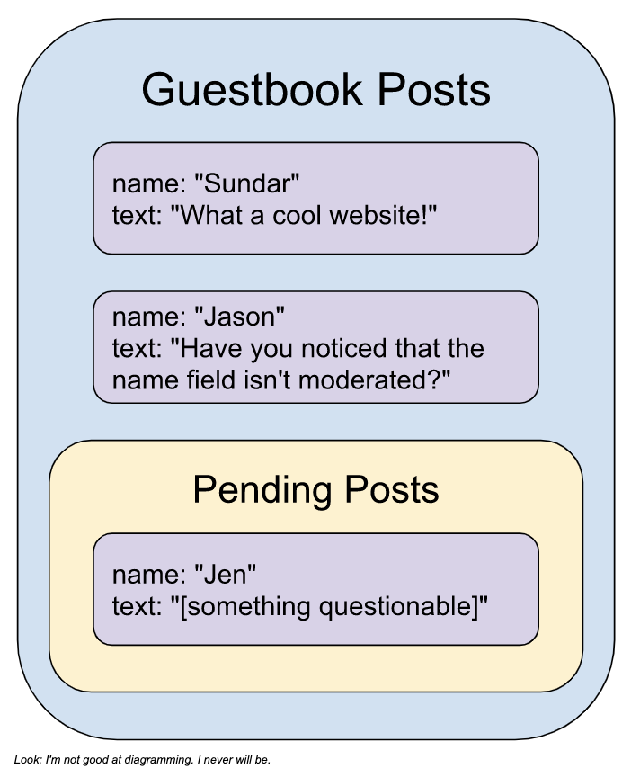
You’ve probably noticed that my moderation functionality doesn’t extend to the name field. This means that even a halfway-clever troll could easily get around the filter by cramming all of their expletives into that name field. That’s a good point and I trust that you will use some type of moderation on all fields that users interact with. Perhaps you use an authentication method to identify users so they aren’t provided a field for their name. Anyway, you get it: I didn’t add moderation to the name field, but in a production environment, you definitely want moderation on all fields.
Build a better fit
When you test out real-world text samples on your website, you might find that the text toxicity classifier model doesn’t quite fit your needs. Since each social space is unique, there will be specific language that you are looking to include and exclude. You can address these needs by training the model on new data that you provide.
If you enjoyed this article and would like to learn more about TensorFlow.js, then there are a ton of things you can do:
- Check out the TensorFlow.js edX course by Jason Mayes. If you are even remotely interested in using TensorFlow.js, I cannot recommend this enough. It might look like a lot at first, but the course is broken up into easy-to-follow manageable pieces.
- View all the TensorFlow.js pretrained models in the TFJS repository on GitHub.
- Play around with TensorFlow.js projects on Glitch.
Automatically optimizing execution of unfamiliar tensor operations
New auto-scheduler speeds optimization process sixfold while improving performance of resulting code up to 70%.Read More
GeForce NOW Supports Over 1,400 Games Streaming Instantly
This GFN Thursday marks a milestone: With the addition of six new titles this week, more than 1,400 games are now available to stream from the GeForce NOW library.
Plus, GeForce NOW members streaming to supported Smart TVs from Samsung and LG can get into their games faster with an improved user interface.
Your Games, Your Way
With more than 1,400 games streaming instantly on GeForce NOW, there’s always something new to play.

Enjoy stunning stories like Mass Effect Legendary Edition or Life is Strange: True Colors, streaming to PCs and even Macs in 4K resolution with an RTX 3080 membership. Group up with friends in Lost Ark or betray them for fun in Among Us. Squad up for victory in Apex Legends, Rocket League and Counter-Strike: Global Offensive — and don’t worry about lagging behind, thanks to ultra-low latency.
For those craving something spooky, have a drop-dead good time ghost hunting in Phasmophobia or struggle to survive and slay in Dead by Daylight. Games like these sound scary good in 5.1 and 7.1 surround sound for Priority and 3080 members.
Build out your library, starting with over 100 free-to-play titles like League of Legends and Rumbleverse. RTX 3080 and Priority members can also experience real-time ray tracing in games like Dying Light 2, Loopmancer and Cyberpunk 2077, which launched a new 1.6 update this week, bringing even more content to Night City.
Take the action on the go with mobile devices. Fortnite on GeForce NOW with touch controls on mobile is available to all members, streaming through the Safari web browser on iOS and the GeForce NOW Android app. Or tap your way through Teyvet in Genshin Impact, streaming to mobile devices with touch controls.
With new games arriving on the cloud every week, the choices are endless.
Stream on TVs
GeForce NOW members streaming to Samsung and LG TVs can now quickly discover and easily launch top games through an improved UI.

Samsung has integrated a “Featured on GeForce NOW” row in the Samsung Gaming Hub, streaming on select 2022 4K TVs. The list is curated and updated regularly — showcasing new, popular and recently released games. GeForce NOW is also integrated into other rows, like “Popular Games,” which Samsung also curates weekly. Pick out a game from these menus and easily launch the GeForce NOW app.

LG updated its UI with a home-screen “Gaming Shelf.” This addition brings GeForce NOW titles right onto the home screen, adding a new layer of game discoverability for members streaming to supported 2022 and 2021 LG TVs. Members with supported TVs can download the GeForce NOW app and check out the new UI today.
Revolutionize the Weekend

Charge into the weekend with six new titles streaming from the cloud:
- Gloomwood (New release on Steam)
- TRAIL OUT (New release on Steam)
- Shatterline (New release on Steam, Sept 8)
- Steelrising (New release on Steam and Epic Games Store, Sept. 8)
- Broken Pieces (New release on Steam, Sept. 9)
- Realm Royale Reforged (Epic Games Store)
What are you planning to play this weekend? Let us know on Twitter or in the comments below.
The post GeForce NOW Supports Over 1,400 Games Streaming Instantly appeared first on NVIDIA Blog.

AI system makes models like DALL-E 2 more creative
The internet had a collective feel-good moment with the introduction of DALL-E, an artificial intelligence-based image generator inspired by artist Salvador Dali and the lovable robot WALL-E that uses natural language to produce whatever mysterious and beautiful image your heart desires. Seeing typed-out inputs like “smiling gopher holding an ice cream cone” instantly spring to life clearly resonated with the world.
Getting said smiling gopher and attributes to pop up on your screen is not a small task. DALL-E 2 uses something called a diffusion model, where it tries to encode the entire text into one description to generate an image. But once the text has a lot of more details, it’s hard for a single description to capture it all. Moreover, while they’re highly flexible, they sometimes struggle to understand the composition of certain concepts, like confusing the attributes or relations between different objects.
To generate more complex images with better understanding, scientists from MIT’s Computer Science and Artificial Intelligence Laboratory (CSAIL) structured the typical model from a different angle: they added a series of models together, where they all cooperate to generate desired images capturing multiple different aspects as requested by the input text or labels. To create an image with two components, say, described by two sentences of description, each model would tackle a particular component of the image.
The seemingly magical models behind image generation work by suggesting a series of iterative refinement steps to get to the desired image. It starts with a “bad” picture and then gradually refines it until it becomes the selected image. By composing multiple models together, they jointly refine the appearance at each step, so the result is an image that exhibits all the attributes of each model. By having multiple models cooperate, you can get much more creative combinations in the generated images.
Take, for example, a red truck and a green house. The model will confuse the concepts of red truck and green house when these sentences get very complicated. A typical generator like DALL-E 2 might make a green truck and a red house, so it’ll swap these colors around. The team’s approach can handle this type of binding of attributes with objects, and especially when there are multiple sets of things, it can handle each object more accurately.
“The model can effectively model object positions and relational descriptions, which is challenging for existing image-generation models. For example, put an object and a cube in a certain position and a sphere in another. DALL-E 2 is good at generating natural images but has difficulty understanding object relations sometimes,” says MIT CSAIL PhD student and co-lead author Shuang Li, “Beyond art and creativity, perhaps we could use our model for teaching. If you want to tell a child to put a cube on top of a sphere, and if we say this in language, it might be hard for them to understand. But our model can generate the image and show them.”
Making Dali proud
Composable Diffusion — the team’s model — uses diffusion models alongside compositional operators to combine text descriptions without further training. The team’s approach more accurately captures text details than the original diffusion model, which directly encodes the words as a single long sentence. For example, given “a pink sky” AND “a blue mountain in the horizon” AND “cherry blossoms in front of the mountain,” the team’s model was able to produce that image exactly, whereas the original diffusion model made the sky blue and everything in front of the mountains pink.
“The fact that our model is composable means that you can learn different portions of the model, one at a time. You can first learn an object on top of another, then learn an object to the right of another, and then learn something left of another,” says co-lead author and MIT CSAIL PhD student Yilun Du. “Since we can compose these together, you can imagine that our system enables us to incrementally learn language, relations, or knowledge, which we think is a pretty interesting direction for future work.”
While it showed prowess in generating complex, photorealistic images, it still faced challenges since the model was trained on a much smaller dataset than those like DALL-E 2, so there were some objects it simply couldn’t capture.
Now that Composable Diffusion can work on top of generative models, such as DALL-E 2, the scientists want to explore continual learning as a potential next step. Given that more is usually added to object relations, they want to see if diffusion models can start to “learn” without forgetting previously learned knowledge — to a place where the model can produce images with both the previous and new knowledge.
“This research proposes a new method for composing concepts in text-to-image generation not by concatenating them to form a prompt, but rather by computing scores with respect to each concept and composing them using conjunction and negation operators,” says Mark Chen, co-creator of DALL-E 2 and research scientist at OpenAI. “This is a nice idea that leverages the energy-based interpretation of diffusion models so that old ideas around compositionality using energy-based models can be applied. The approach is also able to make use of classifier-free guidance, and it is surprising to see that it outperforms the GLIDE baseline on various compositional benchmarks and can qualitatively produce very different types of image generations.”
“Humans can compose scenes including different elements in a myriad of ways, but this task is challenging for computers,” says Bryan Russel, research scientist at Adobe Systems. “This work proposes an elegant formulation that explicitly composes a set of diffusion models to generate an image given a complex natural language prompt.”
Alongside Li and Du, the paper’s co-lead authors are Nan Liu, a master’s student in computer science at the University of Illinois at Urbana-Champaign, and MIT professors Antonio Torralba and Joshua B. Tenenbaum. They will present the work at the 2022 European Conference on Computer Vision.
The research was supported by Raytheon BBN Technologies Corp., Mitsubishi Electric Research Laboratory, and DEVCOM Army Research Laboratory.
My journey from DeepMind intern to mentor
Former intern turned intern manager, Richard Everett, describes his journey to DeepMind, sharing tips and advice for aspiring DeepMinders. The 2023 internship applications will open on the 16th September, please visit https://dpmd.ai/internshipsatdeepmind for more information.Read More