Former intern turned intern manager, Richard Everett, describes his journey to DeepMind, sharing tips and advice for aspiring DeepMinders. The 2023 internship applications will open on the 16th September, please visit https://dpmd.ai/internshipsatdeepmind for more information.Read More

Announcing TensorFlow Official Build Collaborators

Posted by Rostam Dinyari, Nitin Srinivasan, Douglas Yarrington and Rishika Sinha of the TensorFlow team
Starting with TensorFlow 2.10, we are excited to announce our collaboration with Intel, AWS, ARM, and Linaro to develop official TensorFlow builds. This means that when you pip install TensorFlow on Windows Native and Linux Aarch64 hosts, you will receive a build of TensorFlow that has been reviewed and vetted by these platform experts. This happens transparently, and there are no changes to your workflow . We’ve updated the pip install scripts so it’s automatic for you.
Official builds are TensorFlow releases that follow rigorous functional and performance testing standards Google engineers and our collaborators publish with each release, which we align with our published support expectations under the SIG Build forum. Collaborators monitor the builds daily and publish artifacts to the community in coordination with the overall TensorFlow release schedule.
For the majority of use cases, there will be no changes to the behavior of pip install or pip uninstall TensorFlow. However, for Windows Native and Linux Aarch64 based systems an additional pip uninstall step may be needed. You can find details about install, uninstall and other best practices on tensorflow.org/install/pip.
Over time, we expect the number of collaborators to expand but for now we want to share with you the progress we have made together to release increasingly performant and robust builds for these important platforms. You can learn more about each of the collaborations below.
Intel Collaboration
We are pleased to share that Intel has joined the 3P Official Build program to take ownership over Windows Native CPU builds. This will include responsibility for managing both nightly and final production releases. We and Intel do not expect this to disrupt end user experiences; users simply install TensorFlow as usual and the Intel produced Python binary artifacts (wheel files) will be correctly installed.
AWS, ARM and Linaro Collaboration
We are especially pleased to announce the availability of official builds for ARM Aarch64, specifically tuned for AWS Graviton instances. Together, the experts at Linaro have supported Google, AWS and ARM to ensure a highly performant version of TensorFlow is available on the emerging class of Aarch64 devices.
Next steps
These changes should be transparent for most users. You can learn more at tensorflow.org/install.
Transfer learning for TensorFlow image classification models in Amazon SageMaker
Amazon SageMaker provides a suite of built-in algorithms, pre-trained models, and pre-built solution templates to help data scientists and machine learning (ML) practitioners get started on training and deploying ML models quickly. You can use these algorithms and models for both supervised and unsupervised learning. They can process various types of input data, including tabular, image, and text.
Starting today, SageMaker provides a new built-in algorithm for image classification: Image Classification – TensorFlow. It is a supervised learning algorithm that supports transfer learning for many pre-trained models available in TensorFlow Hub. It takes an image as input and outputs probability for each of the class labels. You can fine-tune these pre-trained models using transfer learning even when a large number of training images aren’t available. It’s available through the SageMaker built-in algorithms as well as through the SageMaker JumpStart UI inside Amazon SageMaker Studio. For more information, refer to its documentation Image Classification – TensorFlow and the example notebook Introduction to SageMaker TensorFlow – Image Classification.
Image classification with TensorFlow in SageMaker provides transfer learning on many pre-trained models available in TensorFlow Hub. According to the number of class labels in the training data, a classification layer is attached to the pre-trained TensorFlow Hub model. The classification layer consists of a dropout layer and a dense layer, which is a fully connected layer with 2-norm regularizer that is initialized with random weights. The model training has hyperparameters for the dropout rate of the dropout layer and the L2 regularization factor for the dense layer. Then either the whole network, including the pre-trained model, or only the top classification layer can be fine-tuned on the new training data. In this transfer learning mode, you can achieve training even with a smaller dataset.
How to use the new TensorFlow image classification algorithm
This section describes how to use the TensorFlow image classification algorithm with the SageMaker Python SDK. For information on how to use it from the Studio UI, see SageMaker JumpStart.
The algorithm supports transfer learning for the pre-trained models listed in TensorFlow Hub Models. Each model is identified by a unique model_id. The following code shows how to fine-tune MobileNet V2 1.00 224 identified by model_id tensorflow-ic-imagenet-mobilenet-v2-100-224-classification-4 on a custom training dataset. For each model_id, in order to launch a SageMaker training job through the Estimator class of the SageMaker Python SDK, you need to fetch the Docker image URI, training script URI, and pre-trained model URI through the utility functions provided in SageMaker. The training script URI contains all the necessary code for data processing, loading the pre-trained model, model training, and saving the trained model for inference. The pre-trained model URI contains the pre-trained model architecture definition and the model parameters. Note that the Docker image URI and the training script URI are the same for all the TensorFlow image classification models. The pre-trained model URI is specific to the particular model. The pre-trained model tarballs have been pre-downloaded from TensorFlow Hub and saved with the appropriate model signature in Amazon Simple Storage Service (Amazon S3) buckets, such that the training job runs in network isolation. See the following code:
With these model-specific training artifacts, you can construct an object of the Estimator class:
Next, for transfer learning on your custom dataset, you might need to change the default values of the training hyperparameters, which are listed in Hyperparameters. You can fetch a Python dictionary of these hyperparameters with their default values by calling hyperparameters.retrieve_default, update them as needed, and then pass them to the Estimator class. Note that the default values of some of the hyperparameters are different for different models. For large models, the default batch size is smaller and the train_only_top_layer hyperparameter is set to True. The hyperparameter Train_only_top_layer defines which model parameters change during the fine-tuning process. If train_only_top_layer is True, parameters of the classification layers change and the rest of the parameters remain constant during the fine-tuning process. On the other hand, if train_only_top_layer is False, all parameters of the model are fine-tuned. See the following code:
The following code provides a default training dataset hosted in S3 buckets. We provide the tf_flowers dataset as a default dataset for fine-tuning the models. The dataset comprises images of five types of flowers. The dataset has been downloaded from TensorFlow under the Apache 2.0 License.
Finally, to launch the SageMaker training job for fine-tuning the model, call .fit on the object of the Estimator class, while passing the S3 location of the training dataset:
For more information about how to use the new SageMaker TensorFlow image classification algorithm for transfer learning on a custom dataset, deploy the fine-tuned model, run inference on the deployed model, and deploy the pre-trained model as is without first fine-tuning on a custom dataset, see the following example notebook: Introduction to SageMaker TensorFlow – Image Classification.
Input/output interface for the TensorFlow image classification algorithm
You can fine-tune each of the pre-trained models listed in TensorFlow Hub Models to any given dataset comprising images belonging to any number of classes. The objective is to minimize prediction error on the input data. The model returned by fine-tuning can be further deployed for inference. The following are the instructions for how the training data should be formatted for input to the model:
- Input – A directory with as many sub-directories as the number of classes. Each sub-directory should have images belonging to that class in .jpg, .jpeg, or .png format.
- Output – A fine-tuned model that can be deployed for inference or can be further trained using incremental training. A preprocessing and postprocessing signature is added to the fine-tuned model such that it takes raw .jpg image as input and returns class probabilities. A file mapping class indexes to class labels is saved along with the models.
The input directory should look like the following example if the training data contains images from two classes: roses and dandelion. The S3 path should look like s3://bucket_name/input_directory/. Note the trailing / is required. The names of the folders and roses, dandelion, and the .jpg filenames can be anything. The label mapping file that is saved along with the trained model on the S3 bucket maps the folder names roses and dandelion to the indexes in the list of class probabilities the model outputs. The mapping follows alphabetical ordering of the folder names. In the following example, index 0 in the model output list corresponds to dandelion, and index 1 corresponds to roses.
Inference with the TensorFlow image classification algorithm
The generated models can be hosted for inference and support encoded .jpg, .jpeg, and .png image formats as the application/x-image content type. The input image is resized automatically. The output contains the probability values, the class labels for all classes, and the predicted label corresponding to the class index with the highest probability, encoded in JSON format. The TensorFlow image classification model processes a single image per request and outputs only one line in the JSON. The following is an example of a response in JSON:
If accept is set to application/json, then the model only outputs probabilities. For more details on training and inference, see the sample notebook Introduction to SageMaker TensorFlow – Image Classification.
Use SageMaker built-in algorithms through the JumpStart UI
You can also use SageMaker TensorFlow image classification and any of the other built-in algorithms with a few clicks via the JumpStart UI. JumpStart is a SageMaker feature that allows you to train and deploy built-in algorithms and pre-trained models from various ML frameworks and model hubs through a graphical interface. It also allows you to deploy fully fledged ML solutions that string together ML models and various other AWS services to solve a targeted use case. Check out Run text classification with Amazon SageMaker JumpStart using TensorFlow Hub and Hugging Face models to find out how to use JumpStart to train an algorithm or pre-trained model in a few clicks.
Conclusion
In this post, we announced the launch of the SageMaker TensorFlow image classification built-in algorithm. We provided example code on how to do transfer learning on a custom dataset using a pre-trained model from TensorFlow Hub using this algorithm. For more information, check out documentation and the example notebook.
About the authors
 Dr. Ashish Khetan is a Senior Applied Scientist with Amazon SageMaker built-in algorithms and helps develop machine learning algorithms. He got his PhD from University of Illinois Urbana-Champaign. He is an active researcher in machine learning and statistical inference, and has published many papers in NeurIPS, ICML, ICLR, JMLR, ACL, and EMNLP conferences.
 Dr. Vivek Madan is an Applied Scientist with the Amazon SageMaker JumpStart team. He got his PhD from University of Illinois Urbana-Champaign and was a Post Doctoral Researcher at Georgia Tech. He is an active researcher in machine learning and algorithm design, and has published papers in EMNLP, ICLR, COLT, FOCS, and SODA conferences.
 João Moura is an AI/ML Specialist Solutions Architect at Amazon Web Services. He is mostly focused on NLP use cases and helping customers optimize deep learning model training and deployment. He is also an active proponent of low-code ML solutions and ML-specialized hardware.
 Raju Penmatcha is a Senior AI/ML Specialist Solutions Architect at AWS. He works with education, government, and nonprofit customers on machine learning and artificial intelligence related projects, helping them build solutions using AWS. When not helping customers, he likes traveling to new places.
Improve transcription accuracy of customer-agent calls with custom vocabulary in Amazon Transcribe
Many AWS customers have been successfully using Amazon Transcribe to accurately, efficiently, and automatically convert their customer audio conversations to text, and extract actionable insights from them. These insights can help you continuously enhance the processes and products that directly improve the quality and experience for your customers.
In many countries, such as India, English is not the primary language of communication. Indian customer conversations contain regional languages like Hindi, with English words and phrases spoken randomly throughout the calls. In the source media files, there can be proper nouns, domain-specific acronyms, words, or phrases that the default Amazon Transcribe model isn’t aware of. Transcriptions for such media files can have inaccurate spellings for those words.
In this post, we demonstrate how you can provide more information to Amazon Transcribe with custom vocabularies to update the way Amazon Transcribe handles transcription of your audio files with business-specific terminology. We show the steps to improve the accuracy of transcriptions for Hinglish calls (Indian Hindi calls containing Indian English words and phrases). You can use the same process to transcribe audio calls with any language supported by Amazon Transcribe. After you create custom vocabularies, you can transcribe audio calls with accuracy and at scale by using our post call analytics solution, which we discuss more later in this post.
Solution overview
We use the following Indian Hindi audio call (SampleAudio.wav) with random English words to demonstrate the process.
We then walk you through the following high-level steps:
- Transcribe the audio file using the default Amazon Transcribe Hindi model.
- Measure model accuracy.
- Train the model with custom vocabulary.
- Measure the accuracy of the trained model.
Prerequisites
Before we get started, we need to confirm that the input audio file meets the transcribe data input requirements.
A monophonic recording, also referred to as mono, contains one audio signal, in which all the audio elements of the agent and the customer are combined into one channel. A stereophonic recording, also referred to as stereo, contains two audio signals to capture the audio elements of the agent and the customer in two separate channels. Each agent-customer recording file contains two audio channels, one for the agent and one for the customer.
Low-fidelity audio recordings, such as telephone recordings, typically use 8,000 Hz sample rates. Amazon Transcribe supports processing mono recorded and also high-fidelity audio files with sample rates between 16,000–48,000 Hz.
For improved transcription results and to clearly distinguish the words spoken by the agent and the customer, we recommend using audio files recorded at 8,000 Hz sample rate and are stereo channel separated.
You can use a tool like ffmpeg to validate your input audio files from the command line:
In the returned response, check the line starting with Stream in the Input section, and confirm that the audio files are 8,000 Hz and stereo channel separated:
When you build a pipeline to process a large number of audio files, you can automate this step to filter files that don’t meet the requirements.
As an additional prerequisite step, create an Amazon Simple Storage Service (Amazon S3) bucket to host the audio files to be transcribed. For instructions, refer to Create your first S3 bucket.Then upload the audio file to the S3 bucket.
Transcribe the audio file with the default model
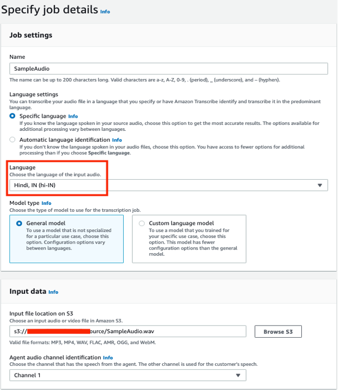
Now we can start an Amazon Transcribe call analytics job using the audio file we uploaded.In this example, we use the AWS Management Console to transcribe the audio file.You can also use the AWS Command Line Interface (AWS CLI) or AWS SDK.
- On the Amazon Transcribe console, choose Call analytics in the navigation pane.
- Choose Call analytics jobs.
- Choose Create job.

- For Name, enter a name.
- For Language settings, select Specific language.
- For Language, choose Hindi, IN (hi-IN).
- For Model type, select General model.
- For Input file location on S3, browse to the S3 bucket containing the uploaded audio file.
- In the Output data section, leave the defaults.
- In the Access permissions section, select Create an IAM role.
- Create a new AWS Identity and Access Management (IAM) role named HindiTranscription that provides Amazon Transcribe service permissions to read the audio files from the S3 bucket and use the AWS Key Management Service (AWS KMS) key to decrypt.

- In the Configure job section, leave the defaults, including Custom vocabulary deselected.
- Choose Create job to transcribe the audio file.

When the status of the job is Complete, you can review the transcription by choosing the job (SampleAudio).

The customer and the agent sentences are clearly separated out, which helps us identify whether the customer or the agent spoke any specific words or phrases.
Measure model accuracy
Word error rate (WER) is the recommended and most commonly used metric for evaluating the accuracy of Automatic Speech Recognition (ASR) systems. The goal is to reduce the WER as much possible to improve the accuracy of the ASR system.
To calculate WER, complete the following steps. This post uses the open-source asr-evaluation evaluation tool to calculate WER, but other tools such as SCTK or JiWER are also available.
-
Install the
asr-evaluationtool, which makes the wer script available on your command line.
Use a command line on macOS or Linux platforms to run the wer commands shown later in the post. - Copy the transcript from the Amazon Transcribe job details page to a text file named
hypothesis.txt.
When you copy the transcription from the console, you’ll notice a new line character between the wordsAgent :, Customer :,and the Hindi script.
The new line characters have been removed to save space in this post. If you choose to use the text as is from the console, make sure that the reference text file you create also has the new line characters, because the wer tool compares line by line. - Review the entire transcript and identify any words or phrases that need to be corrected:
Customer : हेलो,
Agent : गुड मोर्निग इंडिया ट्रेवल एजेंसी सेम है। लावन्या बात कर रही हूँ किस तरह से मैं आपकी सहायता कर सकती हूँ।
Customer : मैं बहुत दिनों उनसे हैदराबाद ट्रेवल के बारे में सोच रहा था। क्या आप मुझे कुछ अच्छे लोकेशन के बारे में बता सकती हैं?
Agent :हाँ बिल्कुल। हैदराबाद में बहुत सारे प्लेस है। उनमें से चार महीना गोलकुंडा फोर सलार जंग म्यूजियम और बिरला प्लेनेटोरियम मशहूर है।
Customer : हाँ बढिया थैंक यू मैं अगले सैटरडे और संडे को ट्राई करूँगा।
Agent : एक सजेशन वीकेंड में ट्रैफिक ज्यादा रहने के चांसेज है।
Customer : सिरियसली एनी टिप्स चिकन शेर
Agent : आप टेक्सी यूस कर लो ड्रैब और पार्किंग का प्राब्लम नहीं होगा।
Customer : ग्रेट आइडिया थैंक्यू सो मच।The highlighted words are the ones that the default Amazon Transcribe model didn’t render correctly. - Create another text file named
reference.txt, replacing the highlighted words with the desired words you expect to see in the transcription:
Customer : हेलो,
Agent : गुड मोर्निग सौथ इंडिया ट्रेवल एजेंसी से मैं । लावन्या बात कर रही हूँ किस तरह से मैं आपकी सहायता कर सकती हूँ।
Customer : मैं बहुत दिनोंसे हैदराबाद ट्रेवल के बारे में सोच रहा था। क्या आप मुझे कुछ अच्छे लोकेशन के बारे में बता सकती हैं?
Agent : हाँ बिल्कुल। हैदराबाद में बहुत सारे प्लेस है। उनमें से चार मिनार गोलकोंडा फोर्ट सालार जंग म्यूजियम और बिरला प्लेनेटोरियम मशहूर है।
Customer : हाँ बढिया थैंक यू मैं अगले सैटरडे और संडे को ट्राई करूँगा।
Agent : एक सजेशन वीकेंड में ट्रैफिक ज्यादा रहने के चांसेज है।
Customer : सिरियसली एनी टिप्स यू केन शेर
Agent : आप टेक्सी यूस कर लो ड्रैव और पार्किंग का प्राब्लम नहीं होगा।
Customer : ग्रेट आइडिया थैंक्यू सो मच। - Use the following command to compare the reference and hypothesis text files that you created:
You get the following output:
The wer command compares text from the files reference.txt and hypothesis.txt. It reports errors for each sentence and also the total number of errors (WER: 9.848% ( 13 / 132)) in the entire transcript.
From the preceding output, wer reported 13 errors out of 132 words in the transcript. These errors can be of three types:
- Substitution errors – These occur when Amazon Transcribe writes one word in place of another. For example, in our transcript, the word “महीना (Mahina)” was written instead of “मिनार (Minar)” in sentence 4.
- Deletion errors – These occur when Amazon Transcribe misses a word entirely in the transcript.In our transcript, the word “सौथ (South)” was missed in sentence 2.
- Insertion errors – These occur when Amazon Transcribe inserts a word that wasn’t spoken. We don’t see any insertion errors in our transcript.
Observations from the transcript created by the default model
We can make the following observations based on the transcript:
- The total WER is 9.848%, meaning 90.152% of the words are transcribed accurately.
- The default Hindi model transcribed most of the English words accurately. This is because the default model is trained to recognize the most common English words out of the box. The model is also trained to recognize Hinglish language, where English words randomly appear in Hindi conversations. For example:
- गुड मोर्निग – Good morning (sentence 2).
- ट्रेवल एजेंसी – Travel agency (sentence 2).
- ग्रेट आइडिया थैंक्यू सो मच – Great idea thank you so much (sentence 9).
- Sentence 4 has the most errors, which are the names of places in the Indian city Hyderabad:
- हाँ बिल्कुल। हैदराबाद में बहुत सारे प्लेस है। उनमें से चार महीना गोलकुंडा फोर सलार जंग म्यूजियम और बिरला प्लेनेटोरियम मशहूर है।
In the next step, we demonstrate how to correct the highlighted words in the preceding sentence using custom vocabulary in Amazon Transcribe:
- चार महीना (Char Mahina) should be चार मिनार (Char Minar)
- गोलकुंडा फोर (Golcunda Four) should be गोलकोंडा फोर्ट (Golconda Fort)
- सलार जंग (Salar Jung) should be सालार जंग (Saalar Jung)
Train the default model with a custom vocabulary
To create a custom vocabulary, you need to build a text file in a tabular format with the words and phrases to train the default Amazon Transcribe model. Your table must contain all four columns (Phrase, SoundsLike, IPA, and DisplayAs), but the Phrase column is the only one that must contain an entry on each row. You can leave the other columns empty. Each column must be separated by a tab character, even if some columns are left empty. For example, if you leave the IPA and SoundsLike columns empty for a row, the Phrase and DisplaysAs columns in that row must be separated with three tab characters (between Phrase and IPA, IPA and SoundsLike, and SoundsLike and DisplaysAs).
To train the model with a custom vocabulary, complete the following steps:
- Create a file named
HindiCustomVocabulary.txtwith the following content.You can only use characters that are supported for your language. Refer to your language’s character set for details.
The columns contain the following information:
-
Phrase– Contains the words or phrases that you want to transcribe accurately. The highlighted words or phrases in the transcript created by the default Amazon Transcribe model appear in this column. These words are generally acronyms, proper nouns, or domain-specific words and phrases that the default model isn’t aware of. This is a mandatory field for every row in the custom vocabulary table. In our transcript, to correct “गोलकुंडा फोर (Golcunda Four)” from sentence 4, use “गोलकुंडा-फोर (Golcunda-Four)” in this column. If your entry contains multiple words, separate each word with a hyphen (-); do not use spaces. -
IPA– Contains the words or phrases representing speech sounds in the written form. The column is optional; you can leave its rows empty. This column is intended for phonetic spellings using only characters in the International Phonetic Alphabet (IPA). Refer to Hindi character set for the allowed IPA characters for the Hindi language. In our example, we’re not using IPA. If you have an entry in this column, yourSoundsLikecolumn must be empty. -
SoundsLike– Contains words or phrases broken down into smaller pieces (typically based on syllables or common words) to provide a pronunciation for each piece based on how that piece sounds. This column is optional; you can leave the rows empty. Only add content to this column if your entry includes a non-standard word, such as a brand name, or to correct a word that is being incorrectly transcribed. In our transcript, to correct “सलार जंग (Salar Jung)” from sentence 4, use “सा-लार-जंग (Saa-lar-jung)” in this column. Do not use spaces in this column. If you have an entry in this column, yourIPAcolumn must be empty. -
DisplaysAs– Contains words or phrases with the spellings you want to see in the transcription output for the words or phrases in thePhrasefield. This column is optional; you can leave the rows empty. If you don’t specify this field, Amazon Transcribe uses the contents of thePhrasefield in the output file. For example, in our transcript, to correct “गोलकुंडा फोर (Golcunda Four)” from sentence 4, use “गोलकोंडा फोर्ट (Golconda Fort)” in this column.
-
-
Upload the text file (
HindiCustomVocabulary.txt) to an S3 bucket.Now we create a custom vocabulary in Amazon Transcribe. - On the Amazon Transcribe console, choose Custom vocabulary in the navigation pane.
- For Name, enter a name.
- For Language, choose Hindi, IN (hi-IN).
- For Vocabulary input source, select S3 location.
- For Vocabulary file location on S3, enter the S3 path of the
HindiCustomVocabulary.txtfile. - Choose Create vocabulary.

- Transcribe the
SampleAudio.wavfile with the custom vocabulary, with the following parameters:- For Job name , enter
SampleAudioCustomVocabulary. - For Language, choose Hindi, IN (hi-IN).
- For Input file location on S3, browse to the location of
SampleAudio.wav. - For IAM role, select Use an existing IAM role and choose the role you created earlier.
- In the Configure job section, select Custom vocabulary and choose the custom vocabulary
HindiCustomVocabulary.
- For Job name , enter
- Choose Create job.

Measure model accuracy after using custom vocabulary
Copy the transcript from the Amazon Transcribe job details page to a text file named hypothesis-custom-vocabulary.txt:
Customer : हेलो,
Agent : गुड मोर्निग इंडिया ट्रेवल एजेंसी सेम है। लावन्या बात कर रही हूँ किस तरह से मैं आपकी सहायता कर सकती हूँ।
Customer : मैं बहुत दिनों उनसे हैदराबाद ट्रेवल के बारे में सोच रहा था। क्या आप मुझे कुछ अच्छे लोकेशन के बारे में बता सकती हैं?
Agent : हाँ बिल्कुल। हैदराबाद में बहुत सारे प्लेस है। उनमें से चार मिनार गोलकोंडा फोर्ट सालार जंग म्यूजियम और बिरला प्लेनेटोरियम मशहूर है।
Customer : हाँ बढिया थैंक यू मैं अगले सैटरडे और संडे को ट्राई करूँगा।
Agent : एक सजेशन वीकेंड में ट्रैफिक ज्यादा रहने के चांसेज है।
Customer : सिरियसली एनी टिप्स चिकन शेर
Agent : आप टेक्सी यूस कर लो ड्रैब और पार्किंग का प्राब्लम नहीं होगा।
Customer : ग्रेट आइडिया थैंक्यू सो मच।
Note that the highlighted words are transcribed as desired.
Run the wer command again with the new transcript:
You get the following output:
Observations from the transcript created with custom vocabulary
The total WER is 6.061%, meaning 93.939% of the words are transcribed accurately.
Let’s compare the wer output for sentence 4 with and without custom vocabulary. The following is without custom vocabulary:
The following is with custom vocabulary:
There are no errors in sentence 4. The names of the places are transcribed accurately with the help of custom vocabulary, thereby reducing the overall WER from 9.848% to 6.061% for this audio file. This means that the accuracy of transcription improved by nearly 4%.
How custom vocabulary improved the accuracy
We used the following custom vocabulary:
Amazon Transcribe checks if there are any words in the audio file that sound like the words mentioned in the Phrase column. Then the model uses the entries in the IPA, SoundsLike, and DisplaysAs columns for those specific words to transcribe with the desired spellings.
With this custom vocabulary, when Amazon Transcribe identifies a word that sounds like “गोलकुंडा-फोर (Golcunda-Four),” it transcribes that word as “गोलकोंडा फोर्ट (Golconda Fort).”
Recommendations
The accuracy of transcription also depends on parameters like the speakers’ pronunciation, overlapping speakers, talking speed, and background noise. Therefore, we recommend that you to follow the process with a variety of calls (with different customers, agents, interruptions, and so on) that cover the most commonly used domain-specific words for you to build a comprehensive custom vocabulary.
In this post, we learned the process to improve accuracy of transcribing one audio call using custom vocabulary. To process thousands of your contact center call recordings every day, you can use post call analytics, a fully automated, scalable, and cost-efficient end-to-end solution that takes care of most of the heavy lifting. You simply upload your audio files to an S3 bucket, and within minutes, the solution provides call analytics like sentiment in a web UI. Post call analytics provides actionable insights to spot emerging trends, identify agent coaching opportunities, and assess the general sentiment of calls.Post call analytics is an open-source solution that you can deploy using AWS CloudFormation.
Note that custom vocabularies don’t use the context in which the words were spoken, they only focus on individual words that you provide. To further improve the accuracy, you can use custom language models. Unlike custom vocabularies, which associate pronunciation with spelling, custom language models learn the context associated with a given word. This includes how and when a word is used, and the relationship a word has with other words. To create a custom language model, you can use the transcriptions derived from the process we learned for a variety of calls, and combine them with content from your websites or user manuals that contains domain-specific words and phrases.
To achieve the highest transcription accuracy with batch transcriptions, you can use custom vocabularies in conjunction with your custom language models.
Conclusion
In this post, we provided detailed steps to accurately process Hindi audio files containing English words using call analytics and custom vocabularies in Amazon Transcribe. You can use these same steps to process audio calls with any language supported by Amazon Transcribe.
After you derive the transcriptions with your desired accuracy, you can improve your agent-customer conversations by training your agents. You can also understand your customer sentiments and trends. With the help of speaker diarization, loudness detection, and vocabulary filtering features in the call analytics, you can identify whether it was the agent or customer who raised their tone or spoke any specific words. You can categorize calls based on domain-specific words, capture actionable insights, and run analytics to improve your products. Finally, you can translate your transcripts to English or other supported languages of your choice using Amazon Translate.
About the Authors
 Sarat Guttikonda is a Sr. Solutions Architect in AWS World Wide Public Sector. Sarat enjoys helping customers automate, manage, and govern their cloud resources without sacrificing business agility. In his free time, he loves building Legos with his son and playing table tennis.
 Lavanya Sood is a Solutions Architect in AWS World Wide Public Sector based out of New Delhi, India. Lavanya enjoys learning new technologies and helping customers in their cloud adoption journey. In her free time, she loves traveling and trying different foods.

Announcing TensorFlow Lite in Google Play Services General Availability

Posted by Bernhard Bauer and Terry Heo, Software Engineers, Google
Today we’re excited to announce that the Google Play services API for TensorFlow Lite is generally available on Android devices. We recommend this distribution as the path to adding custom machine learning to your apps. Last year, we launched a public beta of TensorFlow Lite in Google Play services at Google I/O. Since then, we’ve received lots of feedback and made improvements to the API. Most recently, we added the GPU delegate and Task Library support. Today we’re moving from beta to general availability on billions of Android devices globally.
TensorFlow Lite in Google Play services is already used by Google teams, including ML Kit, serving over a billion monthly active users and running more than 100 billion daily inferences.
TensorFlow Lite is an inference runtime optimized for mobile devices, and now that it’s part of Google Play services, it helps you deliver better ML experiences because it:
- Reduces your app size by up to 5 MB compared to statically bundling TensorFlow Lite with your app
- Uses the same API as available when bundling TF Lite into your app
- Receives regular performance updates in the background so it’s always getting better automatically
Get started by learning how to add TensorFlow Lite in Google Play Services to your Android app.Read More
A game-theoretic approach to provably correct and scalable offline RL
-
Group
Robot Learning Group
Despite increasingly widespread use of machine learning (ML) in all aspects of our lives, a broad class of scenarios still rely on automation designed by people, not artificial intelligence (AI). In real-world applications that involve making sequences of decisions with long-term consequences, from allocating beds in an intensive-care unit to controlling robots, decision-making strategies to this day are carefully crafted by experienced engineers. But what about reinforcement learning (RL), which gave machines supremacy in games as distinct as Ms. PacMan and Pokémon Go? For all its appeal, RL – specifically, its most famous flavor, online RL – has a significant drawback beyond scenarios that can be simulated and have well-defined behavioral rules. Online RL agents learn by trial and error. They need opportunities to try various actions, observe their consequences, and improve as a result. Making wildly suboptimal decisions just for learning’s sake is acceptable when the biggest stake is a premature demise of a computer game character or showing an irrelevant ad to a website visitor. For tasks such as training a self-driving car’s AI, however, it is clearly not an option.
Offline reinforcement learning (RL) is a paradigm for designing agents that can learn from large existing datasets – possibly collected by recording data from existing reliable but suboptimal human-designed strategies – to make sequential decisions. Unlike the conventional online RL, offline RL can learn policies without collecting online data and even without interacting with a simulator. Moreover, since offline RL does not blindly mimic the behaviors seen in data, like imitation learning (an alternate strategy of RL), offline RL does not require expensive expert-quality decision examples, and the learned policy of offline RL can potentially outperform the best data-collection policy. This means, for example, an offline RL agent in principle can learn a competitive driving policy from logged datasets of regular driving behaviors. Therefore, offline RL offers great potential for large-scale deployment and real-world problem solving.
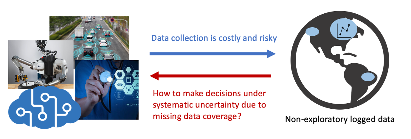
However, offline RL faces a fundamental challenge: the data we can collect in large quantity lacks diversity, so it is impossible to use it to estimate how well a policy would perform in the real world. While we often associate the term “Big Data” with diverse datasets in ML, it is no longer true when the data concerns real-world “sequential” decision making. In fact, curating diverse datasets for these problems can range from difficult to nearly impossible, because it would require running unacceptable experiments in extreme scenarios (like staging the moments just before a car cash, or conducting unethical clinical trials). As a result, the data that gets collected in large quantity, counterintuitively, lacks diversity, which limits its usefulness.
In this post, we introduce a generic game-theoretic framework for offline RL. We frame the offline RL problem as a two-player game where a learning agent competes with an adversary that simulates the uncertain decision outcomes due to missing data coverage. By this game analogy, we design a systematic and provably correct way to design offline RL algorithms that can learn good policies with state-of-the-art empirical performance. Finally, we show that this framework provides a natural connection between offline RL and imitation learning through the lens of generative adversarial networks (GANs). This connection ensures that the policies learned by this game-theoretic framework are always guaranteed to be no worse than the data collection policies. In other words, with this framework, we can use existing data to robustly learn policies that improve upon the human-designed strategies currently running in the system.
The content of this post is based on our recent papers Bellman-consistent Pessimism for Offline Reinforcement Learning (Oral Presentation, NeurIPS 2021) and Adversarially Trained Actor Critic for Offline Reinforcement Learning (Outstanding Paper Runner-up, ICML 2022).
Fundamental difficulty of offline RL and version space
A major limitation of making decisions with only offline data is that existing datasets do not include all possible scenarios in the real world. Hypothetically, suppose that we have a large dataset of how doctors treated patients in the past 50 years, and we want to design an AI agent to make treatment recommendations through RL. If we run a typical RL algorithm on this dataset, the agent might come up with absurd treatments, such as treating a patient with pneumonia through amputation. This is because the dataset does not have examples of what would happen to pneumonia after amputating patients, and “amputation cures pneumonia” may seem to be a plausible scenario to the learning agent, as no information in the data would falsify such a hypothesis.
To address this issue, the agent needs to carefully consider uncertainties due to missing data. Rather than fixating on a particular data-consistent outcome, the agent should be aware of different possibilities (i.e., while amputating the leg might cure the pneumonia, it also might not, since we do not have sufficient evidence for either scenario) before committing to a decision. Such deliberate conservative reasoning is especially important when the agent’s decisions can cause negative consequences in the real world.
A formal way to express the idea above is through the concept of version space. In machine learning, a version space is a set of hypotheses consistent with data. In the context of offline RL, we will form a version space for each candidate decision, describing the possible outcomes if we are to make the decision. Notably, the version space may contain multiple possible outcomes for a candidate decision whose data is missing.
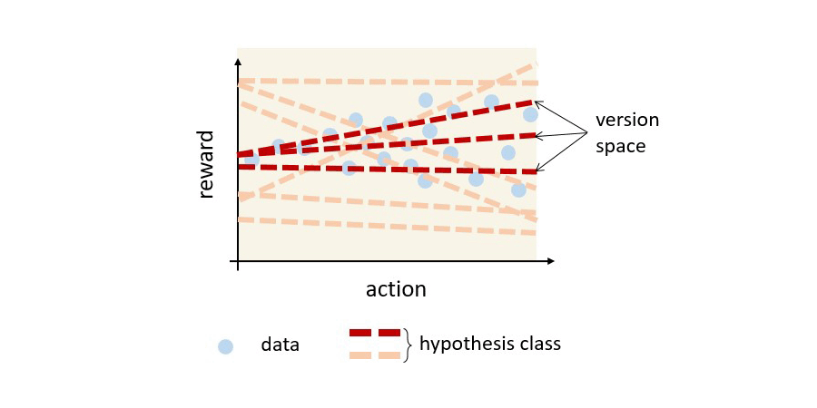
To understand better what a version space is, we use the figure below to visualize the version space of a simplified RL problem where the decision horizon is one. Here we want to select actions that can obtain the highest reward (such as deciding which drug treatment has the highest chance of curing a disease). Suppose we have data of action-reward pairs, and we want to reason about the reward obtained by taking an action. If the underlying reward function is linear, then we have a version space shown in red, which is a subset of (reward) hypotheses that are consistent with the data. In general, for a full RL problem, a version space can be more complicated than just reward functions, e.g., we would need to start thinking about hypotheses about world models or value functions. Nonetheless, similar concepts like the one shown in the figure below apply.
Thinking offline RL as two-player games
If we think about uncertainties as hypotheses in a version space, then a natural strategy of designing offline RL agents is to optimize for the worst-case scenario among all hypotheses in the version space. In this way, the agent would consider all scenarios in the version space as likely, avoiding making decisions following a delusional outcome.
Below we show that this approach of thinking about worst cases for offline RL can be elegantly described by a two-player game, called the Stackelberg game. To this end, let us first introduce some math notations and explain what a Stackelberg game is.
Notation We use (π) to denote a decision policy and use (J(π)) to denote the performance of (π) in the application environment. We use (Π) to denote the set of policies that the learning agent is considering, and we use (mathcal{H}) to denote the set of all hypotheses. We also define a loss function (psi:Π × mathcal{H}→[0, infty)) such that if (psi(π,H)) is small, (H) is a data-consistent hypothesis with respect to (π); conversely (psi(π,H)) gets larger for data-inconsistent ones (e.g., we can treat each (H) as a potential model of the world and (psi(π,H)) as the modelling error on the data). Consequently, a version space above is defined as (mathcal V_pi = { H: psi(pi,H) leq varepsilon }) for some small (varepsilon).
Given a hypothesis (H in mathcal{H}), we use (H(π)) to denote the performance of (π) (predicted) by (H), which may be different from (π)’s true performance (J(π)). As a standard assumption, we suppose for every (π in Π) there is some (H_{π}^* in mathcal{H}) that describes the true outcome of (π), that is, (J(π) = H_{π}^*(π)) and (psi(π,H_{π}^*) = 0).
Stackelberg Game In short, a Stackelberg game is a bilevel optimization problem,
(displaystyle max_{x} f(x,y_x), quad {rm s.t.} ~~ y_x in min_x g(x,y))
In this two-player game, the Leader (x) and the Follower (y) maximize and minimize the payoffs (f) and (g), respectively, under the rule that the Follower plays after the Leader. (This is reflected in the subscript of (y_{x}), that (y) is decided based on the value of (x)). In the special case of (f = g), a Stackelberg game reduces to a zero-sum game (displaystyle max_{x} min_{y} f(x,y)).
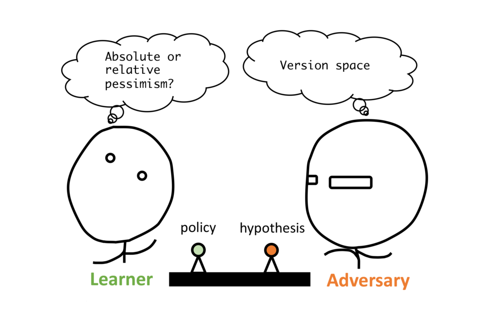
We can think about offline RL as a Stackelberg game: We let the learning agent be the Leader and introduce a fictitious adversary as the Follower, which chooses hypotheses from the version space (V_{π}) based on the Leader’s policy (π). Then we define the payoffs above as performance estimates of a policy in view of a hypothesis. By this construction, solving the Stackelberg would mean finding policies that maximize the worst-case performance, which is exactly our starting goal.
Now we give details on how this game can be designed, using absolute pessimism or relative pessimism, so that we can have performance guarantees in offline RL.
A two-player game based on absolute pessimism
Our first instantiation is a two-player game based on the concept of absolute pessimism, introduced in the paper Bellman-consistent Pessimism for Offline Reinforcement Learning (NeurIPS 2021).
(displaystyle max_{pi in Pi} H_pi(pi), quad {rm s.t.} ~~ H_pi in min_{H in mathcal H} H(pi) + beta psi(pi,H) )
where (beta ge 0) is a hyperparameter which controls how strongly we want the hypothesis to be data consistent. That is, the larger (beta) is, the smaller the version space (mathcal V_pi = { H: psi(pi,H) leq varepsilon }) is (since (varepsilon) is smaller), so we can think that the value of (beta) trades off conservatism and generalization in learning.
This two-player game aims to optimize for the worst-case absolute performance of the agent, as we can treat (H_{π}) as the most pessimistic hypothesis in (mathcal{H}) that is data consistent. Specifically, we can show (H_{π}(π) le J(π)) for any (beta ge 0); as a result, the learner is always optimizing for a performance lower bound.
In addition, we can show that by the design of (psi), this lower bound is tight when (beta) is chosen well (that is, it only underestimates the performance when the policy runs into situations for which we lack data). As a result, with a properly chosen (beta) value, the policy found by the above game formulation is optimal, if the data covers relevant scenarios that an optimal policy would visit, even for data collected by a sub-optimal policy.
In practice, we can define the hypothesis space (mathcal{H}) as a set of value critics (model-free) or world models (model-based). For example, if we set the hypothesis space (mathcal{H}) as candidate Q-functions and (psi) as the Bellman error of a Q function with respect to a policy, then we will get the actor-critic algorithm called PSPI. If we set (mathcal{H}) as candidate models and (psi) as the model fitting error, then we get the CPPO algorithm.
A two-player game based on relative pessimism
While the above game formulation guarantees learning optimality for a well-tuned hyperparameter (beta), the policy performance can be arbitrarily bad if the (beta) value is off. To address this issue, we introduce an alternative two-player game based on relative pessimism, proposed in the paper Adversarially Trained Actor Critic for Offline Reinforcement Learning (ICML 2022).
(displaystyle max_{pi in Pi} H_pi(pi) color{red}{- {H_{π}(mu)}}, {rm s.t.} H_{π} in min_{H in mathcal H} H(π) color{red}{- {H_{π}(mu)}} + betapsi(π,H))
where we use (mu) to denote the data collection policy.
Unlike the absolute pessimism version above, this relative pessimism version is designed to optimize for the worst-case performance relative to the behavior policy (mu). Specifically, we can show (H_pi (pi) – H_pi(mu) leq J(pi) – J(mu)) for all (beta ge 0). And again, we can think about the hypotheses in model-free or model-based manners, like the discussion above. When instantiated model-free, we get the ATAC (Adversarially Trained Actor Critic) algorithm, which achieves state-of-the-art empirical results in offline RL benchmarks.
An important benefit of this relative pessimism version is a robust property to the choice of (beta). As a result, we can guarantee that the learned policy is always no worse than the behavior policy, despite data uncertainty and the (beta) choice – a property we call (robust) (policy) (improvement). The intuition behind this is that (pi = mu) achieves a zero objective in this game, so the agent has an incentive to deviate from (mu) only if it finds a policy (pi) that is uniformly better than (mu) for all possible data-consistent hypotheses.
At the same time, this relative pessimism game is also guaranteed with the learning optimality when (beta) is chosen correctly, just like above absolute pessimism game. Therefore, in some sense, we can view the relative pessimism game (e.g., ATAC) as a robust version of the absolute pessimism game (e.g., PSPI).
A connection between offline RL and imitation learning
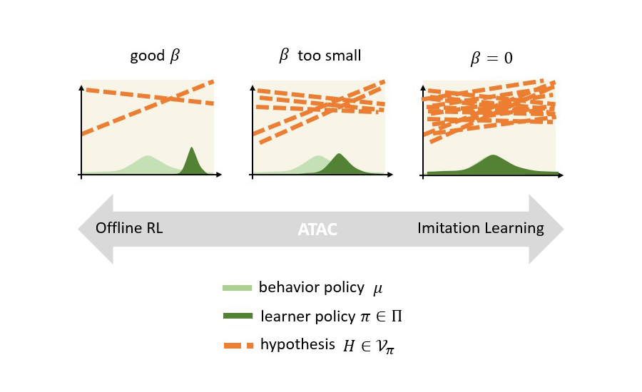
An interesting takeaway from the discussion above is a clean connection between offline RL and imitation learning (IL) based on GANs or integral probability metric. IL like offline RL also tries to learn good policies from offline data. But IL does not use reward information, so the best strategy for IL is to mimic the data collection policy. Among modern IL algorithms, one effective strategy is to use GANs, where we train the policy (the generator) using an adversarial discriminator to separate the actions generated the policy and the actions from the data.
Now that we understand how IL-based on GANs work, we can see the connection between offline RL and IL through the model-free version of the relative pessimism game, that is, ATAC. We can view the actor and the critic of ATAC as the generator and the discriminator in IL based on GANs. By choosing different (beta) values, we can control the strength of the discriminator; when (beta = 0), the discriminator is the strongest, and the best generator is naturally the behavior policy, which recovers the imitation learning behavior. On the other hand, using larger (beta) weakens the discriminator by Bellman regularization (i.e., (psi)) and leads to offline RL.
In conclusion, our game-theoretic framework shows
Offline RL + Relative Pessimism = IL + Bellman Regularization.
We can view them both as solving a version of GANs problems! The only difference is that offline RL uses more restricted discriminators that are consistent with the observed rewards, since the extra information added in offline RL compared with imitation learning is the reward labels.
The high-level takeaway from this connection is that the policies learned by offline RL with the relative pessimism game are guaranteed to be no worse than the data collection policy. In other words, we look forward to exploring possible applications that robustly improve upon existing human-designed strategies running in the system, by just using existing data despite the lack of data diversity.
The post A game-theoretic approach to provably correct and scalable offline RL appeared first on Microsoft Research.
Pinch-grasping robot handles items with precision
Preliminary tests show a prototype pinch-grasping robot achieved a 10-fold reduction in damage on items such as books and boxes.Read More

Collaborative machine learning that preserves privacy
Training a machine-learning model to effectively perform a task, such as image classification, involves showing the model thousands, millions, or even billions of example images. Gathering such enormous datasets can be especially challenging when privacy is a concern, such as with medical images. Researchers from MIT and the MIT-born startup DynamoFL have now taken one popular solution to this problem, known as federated learning, and made it faster and more accurate.
Federated learning is a collaborative method for training a machine-learning model that keeps sensitive user data private. Hundreds or thousands of users each train their own model using their own data on their own device. Then users transfer their models to a central server, which combines them to come up with a better model that it sends back to all users.
A collection of hospitals located around the world, for example, could use this method to train a machine-learning model that identifies brain tumors in medical images, while keeping patient data secure on their local servers.
But federated learning has some drawbacks. Transferring a large machine-learning model to and from a central server involves moving a lot of data, which has high communication costs, especially since the model must be sent back and forth dozens or even hundreds of times. Plus, each user gathers their own data, so those data don’t necessarily follow the same statistical patterns, which hampers the performance of the combined model. And that combined model is made by taking an average — it is not personalized for each user.
The researchers developed a technique that can simultaneously address these three problems of federated learning. Their method boosts the accuracy of the combined machine-learning model while significantly reducing its size, which speeds up communication between users and the central server. It also ensures that each user receives a model that is more personalized for their environment, which improves performance.
The researchers were able to reduce the model size by nearly an order of magnitude when compared to other techniques, which led to communication costs that were between four and six times lower for individual users. Their technique was also able to increase the model’s overall accuracy by about 10 percent.
“A lot of papers have addressed one of the problems of federated learning, but the challenge was to put all of this together. Algorithms that focus just on personalization or communication efficiency don’t provide a good enough solution. We wanted to be sure we were able to optimize for everything, so this technique could actually be used in the real world,” says Vaikkunth Mugunthan PhD ’22, lead author of a paper that introduces this technique.
Mugunthan wrote the paper with his advisor, senior author Lalana Kagal, a principal research scientist in the Computer Science and Artificial Intelligence Laboratory (CSAIL). The work will be presented at the European Conference on Computer Vision.
Cutting a model down to size
The system the researchers developed, called FedLTN, relies on an idea in machine learning known as the lottery ticket hypothesis. This hypothesis says that within very large neural network models there exist much smaller subnetworks that can achieve the same performance. Finding one of these subnetworks is akin to finding a winning lottery ticket. (LTN stands for “lottery ticket network.”)
Neural networks, loosely based on the human brain, are machine-learning models that learn to solve problems using interconnected layers of nodes, or neurons.
Finding a winning lottery ticket network is more complicated than a simple scratch-off. The researchers must use a process called iterative pruning. If the model’s accuracy is above a set threshold, they remove nodes and the connections between them (just like pruning branches off a bush) and then test the leaner neural network to see if the accuracy remains above the threshold.
Other methods have used this pruning technique for federated learning to create smaller machine-learning models which could be transferred more efficiently. But while these methods may speed things up, model performance suffers.
Mugunthan and Kagal applied a few novel techniques to accelerate the pruning process while making the new, smaller models more accurate and personalized for each user.
They accelerated pruning by avoiding a step where the remaining parts of the pruned neural network are “rewound” to their original values. They also trained the model before pruning it, which makes it more accurate so it can be pruned at a faster rate, Mugunthan explains.
To make each model more personalized for the user’s environment, they were careful not to prune away layers in the network that capture important statistical information about that user’s specific data. In addition, when the models were all combined, they made use of information stored in the central server so it wasn’t starting from scratch for each round of communication.
They also developed a technique to reduce the number of communication rounds for users with resource-constrained devices, like a smart phone on a slow network. These users start the federated learning process with a leaner model that has already been optimized by a subset of other users.
Winning big with lottery ticket networks
When they put FedLTN to the test in simulations, it led to better performance and reduced communication costs across the board. In one experiment, a traditional federated learning approach produced a model that was 45 megabytes in size, while their technique generated a model with the same accuracy that was only 5 megabytes. In another test, a state-of-the-art technique required 12,000 megabytes of communication between users and the server to train one model, whereas FedLTN only required 4,500 megabytes.
With FedLTN, the worst-performing clients still saw a performance boost of more than 10 percent. And the overall model accuracy beat the state-of-the-art personalization algorithm by nearly 10 percent, Mugunthan adds.
Now that they have developed and finetuned FedLTN, Mugunthan is working to integrate the technique into a federated learning startup he recently founded, DynamoFL.
Moving forward, he hopes to continue enhancing this method. For instance, the researchers have demonstrated success using datasets that had labels, but a greater challenge would be applying the same techniques to unlabeled data, he says.
Mugunthan is hopeful this work inspires other researchers to rethink how they approach federated learning.
“This work shows the importance of thinking about these problems from a holistic aspect, and not just individual metrics that have to be improved. Sometimes, improving one metric can actually cause a downgrade in the other metrics. Instead, we should be focusing on how we can improve a bunch of things together, which is really important if it is to be deployed in the real world,” he says.
ASpanFormer: Detector-Free Image Matching with Adaptive Span Transformer
Generating robust and reliable correspondences across images is a fundamental task for a diversity of applications. To capture context at both global and local granularity, we propose ASpanFormer, a Transformer-based detector-free matcher that is built on hierarchical attention structure, adopting a novel attention operation which is capable of adjusting attention span in a self-adaptive manner. To achieve this goal, first, flow maps are regressed in each cross attention phase to locate the center of search region. Next, a sampling grid is generated around the center, whose size, instead of…Apple Machine Learning Research